Third Edition
Data
Structures
and Algorithm
Analysis in
Boston Columbus Indianapolis New York San Francisco Upper Saddle River Amsterdam Cape Town Dubai London Madrid Milan Munich Paris Montreal Toronto
Delhi Mexico City Sao Paulo Sydney Hong Kong Seoul Singapore Taipei Tokyo
Third Edition
Data
Structures
and Algorithm
Analysis in
Java
Mark A l l e n W e i s s
Florida International University
PEARSON
Editorial Director: Marcia Horton Project Manager: Pat Brown
Editor-in-Chief: Michael Hirsch Manufacturing Buyer: Pat Brown
Editorial Assistant: Emma Snider Art Director: Jayne Conte Director of Marketing: Patrice Jones Cover Designer: Bruce Kenselaar
Marketing Manager: Yezan Alayan Cover Photo: cDe-Kay Dreamstime.com
Marketing Coordinator: Kathryn Ferranti Media Editor: Daniel Sandin
Director of Production: Vince O’Brien Full-Service Project Management: Integra
Managing Editor: Jeff Holcomb Composition: Integra
Production Project Manager: Kayla Printer/Binder: Courier Westford
Smith-Tarbox Cover Printer: Lehigh-Phoenix Color/Hagerstown
Text Font: Berkeley-Book
Copyright c2012, 2007, 1999 Pearson Education, Inc.,publishing as Addison-Wesley. All rights reserved. Printed in the United States of America. This publication is protected by Copyright, and permission should be obtained from the publisher prior to any prohibited reproduction, storage in a retrieval system, or trans-mission in any form or by any means, electronic, mechanical, photocopying, recording, or likewise. To obtain permission(s) to use material from this work, please submit a written request to Pearson Education, Inc., Permissions Department, One Lake Street, Upper Saddle River, New Jersey 07458, or you may fax your request to 201-236-3290.
Many of the designations by manufacturers and sellers to distinguish their products are claimed as trade-marks. Where those designations appear in this book, and the publisher was aware of a trademark claim, the designations have been printed in initial caps or all caps.
Library of Congress Cataloging-in-Publication Data
Weiss, Mark Allen.
Data structures and algorithm analysis in Java / Mark Allen Weiss. – 3rd ed. p. cm.
ISBN-13: 978-0-13-257627-7 (alk. paper) ISBN-10: 0-13-257627-9 (alk. paper)
1. Java (Computer program language) 2. Data structures (Computer science) 3. Computer algorithms. I. Title.
QA76.73.J38W448 2012
005.1–dc23 2011035536
15 14 13 12 11—CRW—10 9 8 7 6 5 4 3 2 1
C O N T E N T S
Preface xvii
Chapter 1 Introduction
1
1.1 What’s the Book About? 1 1.2 Mathematics Review 2
1.2.1 Exponents 3 1.2.2 Logarithms 3 1.2.3 Series 4
1.2.4 Modular Arithmetic 5 1.2.5 ThePWord 6
1.3 A Brief Introduction to Recursion 8
1.4 Implementing Generic Components Pre-Java 5 12 1.4.1 UsingObjectfor Genericity 13
1.4.2 Wrappers for Primitive Types 14 1.4.3 Using Interface Types for Genericity 14 1.4.4 Compatibility of Array Types 16
1.5 Implementing Generic Components Using Java 5 Generics 16 1.5.1 Simple Generic Classes and Interfaces 17
1.5.2 Autoboxing/Unboxing 18 1.5.3 The Diamond Operator 18 1.5.4 Wildcards with Bounds 19 1.5.5 Generic Static Methods 20 1.5.6 Type Bounds 21
1.5.7 Type Erasure 22
1.5.8 Restrictions on Generics 23
viii Contents
1.6 Function Objects 24 Summary 26
Exercises 26 References 28
Chapter 2 Algorithm Analysis
29
2.1 Mathematical Background 292.2 Model 32
2.3 What to Analyze 33
2.4 Running Time Calculations 35 2.4.1 A Simple Example 36 2.4.2 General Rules 36
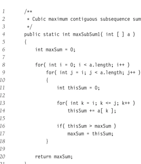
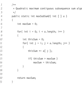
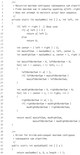
2.4.3 Solutions for the Maximum Subsequence Sum Problem 39 2.4.4 Logarithms in the Running Time 45
2.4.5 A Grain of Salt 49 Summary 49
Exercises 50 References 55
Chapter 3 Lists, Stacks, and Queues
57
3.1 Abstract Data Types (ADTs) 573.2 The List ADT 58
3.2.1 Simple Array Implementation of Lists 58 3.2.2 Simple Linked Lists 59
3.3 Lists in the Java Collections API 61 3.3.1 CollectionInterface 61 3.3.2 Iterators 61
3.3.3 TheListInterface,ArrayList, andLinkedList 63 3.3.4 Example: Usingremoveon aLinkedList 65 3.3.5 ListIterators 67
3.4 Implementation of ArrayList 67 3.4.1 The Basic Class 68
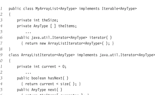
3.4.2 The Iterator and Java Nested and Inner Classes 71 3.5 Implementation of LinkedList 75
Contents ix
3.6.2 Implementation of Stacks 83 3.6.3 Applications 84
3.7 The Queue ADT 92 3.7.1 Queue Model 92
3.7.2 Array Implementation of Queues 92 3.7.3 Applications of Queues 95
Summary 96 Exercises 96
Chapter 4 Trees
101
4.1 Preliminaries 101
4.1.1 Implementation of Trees 102
4.1.2 Tree Traversals with an Application 103 4.2 Binary Trees 107
4.2.1 Implementation 108
4.2.2 An Example: Expression Trees 109 4.3 The Search Tree ADT—Binary Search Trees 112
4.3.1 contains 113
4.3.2 findMinandfindMax 115 4.3.3 insert 116
4.3.4 remove 118
4.3.5 Average-Case Analysis 120 4.4 AVL Trees 123
4.4.1 Single Rotation 125 4.4.2 Double Rotation 128 4.5 Splay Trees 137
4.5.1 A Simple Idea (That Does Not Work) 137 4.5.2 Splaying 139
4.6 Tree Traversals (Revisited) 145 4.7 B-Trees 147
4.8 Sets and Maps in the Standard Library 152 4.8.1 Sets 152
4.8.2 Maps 153
4.8.3 Implementation ofTreeSetandTreeMap 153 4.8.4 An Example That Uses Several Maps 154 Summary 160
x Contents
Chapter 5 Hashing
171
5.1 General Idea 171 5.2 Hash Function 172 5.3 Separate Chaining 174
5.4 Hash Tables Without Linked Lists 179 5.4.1 Linear Probing 179
5.4.2 Quadratic Probing 181 5.4.3 Double Hashing 183 5.5 Rehashing 188
5.6 Hash Tables in the Standard Library 189 5.7 Hash Tables with Worst-CaseO(1) Access 192
5.7.1 Perfect Hashing 193 5.7.2 Cuckoo Hashing 195 5.7.3 Hopscotch Hashing 205 5.8 Universal Hashing 211 5.9 Extendible Hashing 214
Summary 217 Exercises 218 References 222
Chapter 6 Priority Queues (Heaps)
225
6.1 Model 2256.2 Simple Implementations 226 6.3 Binary Heap 226
6.3.1 Structure Property 227 6.3.2 Heap-Order Property 229 6.3.3 Basic Heap Operations 229 6.3.4 Other Heap Operations 234 6.4 Applications of Priority Queues 238
6.4.1 The Selection Problem 238 6.4.2 Event Simulation 239 6.5 d-Heaps 240
6.6 Leftist Heaps 241
Contents xi
6.8 Binomial Queues 252
6.8.1 Binomial Queue Structure 252 6.8.2 Binomial Queue Operations 253
6.8.3 Implementation of Binomial Queues 256 6.9 Priority Queues in the Standard Library 261
Summary 261 Exercises 263 References 267
Chapter 7 Sorting
271
7.1 Preliminaries 271 7.2 Insertion Sort 272
7.2.1 The Algorithm 272
7.2.2 Analysis of Insertion Sort 272
7.3 A Lower Bound for Simple Sorting Algorithms 273 7.4 Shellsort 274
7.4.1 Worst-Case Analysis of Shellsort 276 7.5 Heapsort 278
7.5.1 Analysis of Heapsort 279 7.6 Mergesort 282
7.6.1 Analysis of Mergesort 284 7.7 Quicksort 288
7.7.1 Picking the Pivot 290 7.7.2 Partitioning Strategy 292 7.7.3 Small Arrays 294
7.7.4 Actual Quicksort Routines 294 7.7.5 Analysis of Quicksort 297
7.7.6 A Linear-Expected-Time Algorithm for Selection 300 7.8 A General Lower Bound for Sorting 302
7.8.1 Decision Trees 302
7.9 Decision-Tree Lower Bounds for Selection Problems 304 7.10 Adversary Lower Bounds 307
7.11 Linear-Time Sorts: Bucket Sort and Radix Sort 310 7.12 External Sorting 315
xii Contents
7.12.4 Multiway Merge 317 7.12.5 Polyphase Merge 318 7.12.6 Replacement Selection 319 Summary 321
Exercises 321 References 327
Chapter 8 The Disjoint Set Class
331
8.1 Equivalence Relations 3318.2 The Dynamic Equivalence Problem 332 8.3 Basic Data Structure 333
8.4 Smart Union Algorithms 337 8.5 Path Compression 340
8.6 Worst Case for Union-by-Rank and Path Compression 341 8.6.1 Slowly Growing Functions 342
8.6.2 An Analysis By Recursive Decomposition 343 8.6.3 AnO(Mlog *N) Bound 350
8.6.4 AnO(Mα(M, N) ) Bound 350 8.7 An Application 352
Summary 355 Exercises 355 References 357
Chapter 9 Graph Algorithms
359
9.1 Definitions 359
9.1.1 Representation of Graphs 360 9.2 Topological Sort 362
9.3 Shortest-Path Algorithms 366 9.3.1 Unweighted Shortest Paths 367 9.3.2 Dijkstra’s Algorithm 372
9.3.3 Graphs with Negative Edge Costs 380 9.3.4 Acyclic Graphs 380
9.3.5 All-Pairs Shortest Path 384 9.3.6 Shortest-Path Example 384 9.4 Network Flow Problems 386
Contents xiii
9.5 Minimum Spanning Tree 393 9.5.1 Prim’s Algorithm 394 9.5.2 Kruskal’s Algorithm 397
9.6 Applications of Depth-First Search 399 9.6.1 Undirected Graphs 400
9.6.2 Biconnectivity 402 9.6.3 Euler Circuits 405 9.6.4 Directed Graphs 409
9.6.5 Finding Strong Components 411 9.7 Introduction to NP-Completeness 412
9.7.1 Easy vs. Hard 413 9.7.2 The Class NP 414
9.7.3 NP-Complete Problems 415 Summary 417
Exercises 417 References 425
Chapter 10 Algorithm Design
Techniques
429
10.1 Greedy Algorithms 429
10.1.1 A Simple Scheduling Problem 430 10.1.2 Huffman Codes 433
10.1.3 Approximate Bin Packing 439 10.2 Divide and Conquer 448
10.2.1 Running Time of Divide-and-Conquer Algorithms 449 10.2.2 Closest-Points Problem 451
10.2.3 The Selection Problem 455
10.2.4 Theoretical Improvements for Arithmetic Problems 458 10.3 Dynamic Programming 462
10.3.1 Using a Table Instead of Recursion 463 10.3.2 Ordering Matrix Multiplications 466 10.3.3 Optimal Binary Search Tree 469 10.3.4 All-Pairs Shortest Path 472 10.4 Randomized Algorithms 474
10.4.1 Random Number Generators 476 10.4.2 Skip Lists 480
xiv Contents
10.5 Backtracking Algorithms 486
10.5.1 The Turnpike Reconstruction Problem 487 10.5.2 Games 490
Summary 499 Exercises 499 References 508
Chapter 11 Amortized Analysis
513
11.1 An Unrelated Puzzle 51411.2 Binomial Queues 514 11.3 Skew Heaps 519 11.4 Fibonacci Heaps 522
11.4.1 Cutting Nodes in Leftist Heaps 522 11.4.2 Lazy Merging for Binomial Queues 525 11.4.3 The Fibonacci Heap Operations 528 11.4.4 Proof of the Time Bound 529 11.5 Splay Trees 531
Summary 536 Exercises 536 References 538
Chapter 12 Advanced Data Structures
and Implementation
541
12.1 Top-Down Splay Trees 541 12.2 Red-Black Trees 549
12.2.1 Bottom-Up Insertion 549 12.2.2 Top-Down Red-Black Trees 551 12.2.3 Top-Down Deletion 556 12.3 Treaps 558
12.4 Suffix Arrays and Suffix Trees 560 12.4.1 Suffix Arrays 561
12.4.2 Suffix Trees 564
Contents xv
12.6 Pairing Heaps 583 Summary 588 Exercises 590 References 594
P R E F A C E
Purpose/Goals
This new Java edition describesdata structures, methods of organizing large amounts of data, andalgorithm analysis,the estimation of the running time of algorithms. As computers become faster and faster, the need for programs that can handle large amounts of input becomes more acute. Paradoxically, this requires more careful attention to efficiency, since inefficiencies in programs become most obvious when input sizes are large. By analyzing an algorithm before it is actually coded, students can decide if a particular solution will be feasible. For example, in this text students look at specific problems and see how careful implementations can reduce the time constraint for large amounts of data from centuries to less than a second. Therefore, no algorithm or data structure is presented without an explanation of its running time. In some cases, minute details that affect the running time of the implementation are explored.
Once a solution method is determined, a program must still be written. As computers have become more powerful, the problems they must solve have become larger and more complex, requiring development of more intricate programs. The goal of this text is to teach students good programming and algorithm analysis skills simultaneously so that they can develop such programs with the maximum amount of efficiency.
This book is suitable for either an advanced data structures (CS7) course or a first-year graduate course in algorithm analysis. Students should have some knowledge of intermedi-ate programming, including such topics as object-based programming and recursion, and some background in discrete math.
Summary of the Most Significant Changes in the Third Edition
The third edition incorporates numerous bug fixes, and many parts of the book have undergone revision to increase the clarity of presentation. In addition,
rChapter 4 includes implementation of the AVL tree deletion algorithm—a topic often
requested by readers.
rChapter 5 has been extensively revised and enlarged and now contains material on two
newer algorithms: cuckoo hashing and hopscotch hashing. Additionally, a new section on universal hashing has been added.
rChapter 7 now contains material on radix sort, and a new section on lower bound
xviii Preface
rChapter 8 uses the new union/find analysis by Seidel and Sharir, and shows the O(Mα(M,N) ) bound instead of the weakerO(Mlog∗N) bound in prior editions.
rChapter 12 adds material on suffix trees and suffix arrays, including the linear-time
suffix array construction algorithm by Karkkainen and Sanders (with implementation). The sections covering deterministic skip lists and AA-trees have been removed.
rThroughout the text, the code has been updated to use the diamond operator from
Java 7.
Approach
Although the material in this text is largely language independent, programming requires the use of a specific language. As the title implies, we have chosen Java for this book.
Java is often examined in comparison with C++. Java offers many benefits, and pro-grammers often view Java as a safer, more portable, and easier-to-use language than C++. As such, it makes a fine core language for discussing and implementing fundamental data structures. Other important parts of Java, such as threads and its GUI, although important, are not needed in this text and thus are not discussed.
Complete versions of the data structures, in both Java and C++, are available on the Internet. We use similar coding conventions to make the parallels between the two languages more evident.
Overview
Chapter 1 contains review material on discrete math and recursion. I believe the only way to be comfortable with recursion is to see good uses over and over. Therefore, recursion is prevalent in this text, with examples in every chapter except Chapter 5. Chapter 1 also presents material that serves as a review of inheritance in Java. Included is a discussion of Java generics.
Chapter 2 deals with algorithm analysis. This chapter explains asymptotic analysis and its major weaknesses. Many examples are provided, including an in-depth explanation of logarithmic running time. Simple recursive programs are analyzed by intuitively converting them into iterative programs. More complicated divide-and-conquer programs are intro-duced, but some of the analysis (solving recurrence relations) is implicitly delayed until Chapter 7, where it is performed in detail.
Chapter 3 covers lists, stacks, and queues. This chapter has been significantly revised from prior editions. It now includes a discussion of the Collections API ArrayList
and LinkedList classes, and it provides implementations of a significant subset of the collections APIArrayListandLinkedListclasses.
Preface xix
Chapter 5 discusses hash tables, including the classic algorithms such as sepa-rate chaining and linear and quadratic probing, as well as several newer algorithms, namely cuckoo hashing and hopscotch hashing. Universal hashing is also discussed, and extendible hashing is covered at the end of the chapter.
Chapter 6 is about priority queues. Binary heaps are covered, and there is additional material on some of the theoretically interesting implementations of priority queues. The Fibonacci heap is discussed in Chapter 11, and the pairing heap is discussed in Chapter 12. Chapter 7 covers sorting. It is very specific with respect to coding details and analysis. All the important general-purpose sorting algorithms are covered and compared. Four algorithms are analyzed in detail: insertion sort, Shellsort, heapsort, and quicksort. New to this edition is radix sort and lower bound proofs for selection-related problems. External sorting is covered at the end of the chapter.
Chapter 8 discusses the disjoint set algorithm with proof of the running time. The anal-ysis is new. This is a short and specific chapter that can be skipped if Kruskal’s algorithm is not discussed.
Chapter 9 covers graph algorithms. Algorithms on graphs are interesting, not only because they frequently occur in practice, but also because their running time is so heavily dependent on the proper use of data structures. Virtually all the standard algorithms are presented along with appropriate data structures, pseudocode, and analysis of running time. To place these problems in a proper context, a short discussion on complexity theory (includingNP-completeness and undecidability) is provided.
Chapter 10 covers algorithm design by examining common problem-solving tech-niques. This chapter is heavily fortified with examples. Pseudocode is used in these later chapters so that the student’s appreciation of an example algorithm is not obscured by implementation details.
Chapter 11 deals with amortized analysis. Three data structures from Chapters 4 and 6 and the Fibonacci heap, introduced in this chapter, are analyzed.
Chapter 12 covers search tree algorithms, the suffix tree and array, thek-d tree, and the pairing heap. This chapter departs from the rest of the text by providing complete and careful implementations for the search trees and pairing heap. The material is structured so that the instructor can integrate sections into discussions from other chapters. For exam-ple, the top-down red-black tree in Chapter 12 can be discussed along with AVL trees (in Chapter 4).
Chapters 1–9 provide enough material for most one-semester data structures courses. If time permits, then Chapter 10 can be covered. A graduate course on algorithm analysis could cover Chapters 7–11. The advanced data structures analyzed in Chapter 11 can easily be referred to in the earlier chapters. The discussion ofNP-completeness in Chapter 9 is far too brief to be used in such a course. You might find it useful to use an additional work onNP-completeness to augment this text.
Exercises
xx Preface
References
References are placed at the end of each chapter. Generally the references either are his-torical, representing the original source of the material, or they represent extensions and improvements to the results given in the text. Some references represent solutions to exercises.
Supplements
The following supplements are available to all readers at www.pearsonhighered.com/cssupport:
rSource code for example programs
In addition, the following material is available only to qualified instructors at Pearson’s Instructor Resource Center (www.pearsonhighered.com/irc). Visit the IRC or contact your campus Pearson representative for access.
rSolutions to selected exercises rFigures from the book
Acknowledgments
Many, many people have helped me in the preparation of books in this series. Some are listed in other versions of the book; thanks to all.
As usual, the writing process was made easier by the professionals at Pearson. I’d like to thank my editor, Michael Hirsch, and production editor, Pat Brown. I’d also like to thank Abinaya Rajendran and her team in Integra Software Services for their fine work putting the final pieces together. My wonderful wife Jill deserves extra special thanks for everything she does.
Finally, I’d like to thank the numerous readers who have sent e-mail messages and pointed out errors or inconsistencies in earlier versions. My World Wide Web page www.cis.fiu.edu/~weiss contains updated source code (in Java and C++), an errata list, and a link to submit bug reports.
C H A P T E R
1
Introduction
In this chapter, we discuss the aims and goals of this text and briefly review programming concepts and discrete mathematics. We will
rSee that how a program performs for reasonably large input is just as important as its performance on moderate amounts of input.
rSummarize the basic mathematical background needed for the rest of the book. rBriefly review recursion.
rSummarize some important features of Java that are used throughout the text.
1.1 What’s the Book About?
Suppose you have a group ofNnumbers and would like to determine thekth largest. This is known as theselection problem. Most students who have had a programming course or two would have no difficulty writing a program to solve this problem. There are quite a few “obvious” solutions.
One way to solve this problem would be to read theNnumbers into an array, sort the array in decreasing order by some simple algorithm such as bubblesort, and then return the element in positionk.
A somewhat better algorithm might be to read the firstkelements into an array and sort them (in decreasing order). Next, each remaining element is read one by one. As a new element arrives, it is ignored if it is smaller than thekth element in the array. Otherwise, it is placed in its correct spot in the array, bumping one element out of the array. When the algorithm ends, the element in thekth position is returned as the answer.
Both algorithms are simple to code, and you are encouraged to do so. The natural ques-tions, then, are which algorithm is better and, more important, is either algorithm good enough? A simulation using a random file of 30 million elements andk = 15,000,000 will show that neither algorithm finishes in a reasonable amount of time; each requires several days of computer processing to terminate (albeit eventually with a correct answer). An alternative method, discussed in Chapter 7, gives a solution in about a second. Thus, although our proposed algorithms work, they cannot be considered good algorithms, because they are entirely impractical for input sizes that a third algorithm can handle in a reasonable amount of time.
2 Chapter 1 Introduction
1 2 3 4
1 t h i s
2 w a t s
3 o a h g
4 f g d t
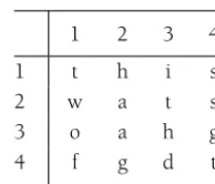
Figure 1.1 Sample word puzzle
A second problem is to solve a popular word puzzle. The input consists of a two-dimensional array of letters and a list of words. The object is to find the words in the puzzle. These words may be horizontal, vertical, or diagonal in any direction. As an example, the puzzle shown in Figure 1.1 contains the wordsthis, two, fat,andthat.The wordthisbegins at row 1, column 1, or (1,1), and extends to (1,4);twogoes from (1,1) to (3,1);fatgoes from (4,1) to (2,3); andthatgoes from (4,4) to (1,1).
Again, there are at least two straightforward algorithms that solve the problem. For each word in the word list, we check each ordered triple (row, column, orientation) for the presence of the word. This amounts to lots of nested for loops but is basically straightforward.
Alternatively, for each ordered quadruple (row, column, orientation, number of characters) that doesn’t run off an end of the puzzle, we can test whether the word indicated is in the word list. Again, this amounts to lots of nestedforloops. It is possible to save some time if the maximum number of characters in any word is known.
It is relatively easy to code up either method of solution and solve many of the real-life puzzles commonly published in magazines. These typically have 16 rows, 16 columns, and 40 or so words. Suppose, however, we consider the variation where only the puzzle board is given and the word list is essentially an English dictionary. Both of the solutions proposed require considerable time to solve this problem and therefore are not acceptable. However, it is possible, even with a large word list, to solve the problem in a matter of seconds.
An important concept is that, in many problems, writing a working program is not good enough. If the program is to be run on a large data set, then the running time becomes an issue. Throughout this book we will see how to estimate the running time of a program for large inputs and, more important, how to compare the running times of two programs without actually coding them. We will see techniques for drastically improving the speed of a program and for determining program bottlenecks. These techniques will enable us to find the section of the code on which to concentrate our optimization efforts.
1.2 Mathematics Review
1.2 Mathematics Review 3
1.2.1 Exponents
XAXB=XA+B XA
XB =X A−B
(XA)B=XAB
XN+XN=2XN=X2N
2N+2N=2N+1
1.2.2 Logarithms
In computer science, all logarithms are to the base 2 unless specified otherwise.
Definition 1.1.
XA=Bif and only if logXB=A
Several convenient equalities follow from this definition.
Theorem 1.1.
logAB= logCB
logCA; A,B,C>0, A=1
Proof.
LetX =logCB, Y =logCA,and Z = logAB. Then, by the definition of logarithms, CX = B,CY = A, andAZ = B. Combining these three equalities yields CX = B = (CY)Z. Therefore,X=YZ,which impliesZ=X/Y, proving the theorem.
Theorem 1.2.
logAB=logA+logB; A,B>0
Proof.
LetX = logA,Y = logB, andZ = logAB. Then, assuming the default base of 2, 2X=A, 2Y = B, and 2Z = AB. Combining the last three equalities yields 2X2Y = AB=2Z. Therefore,X+Y=Z, which proves the theorem.
Some other useful formulas, which can all be derived in a similar manner, follow.
logA/B=logA−logB
log(AB)=BlogA
logX<X for allX>0
4 Chapter 1 Introduction
1.2.3 Series
The easiest formulas to remember are
N
i=0
2i=2N+1−1
and the companion,
N
i=0 Ai= A
N+1−1 A−1
In the latter formula, if 0<A<1, then
N
i=0
Ai≤ 1 1−A
and asN tends to∞, the sum approaches 1/(1−A). These are the “geometric series” formulas.
We can derive the last formula for∞i=0Ai(0<A<1) in the following manner. Let Sbe the sum. Then
S=1+A+A2+A3+A4+A5+ · · ·
Then
AS=A+A2+A3+A4+A5+ · · ·
If we subtract these two equations (which is permissible only for a convergent series), virtually all the terms on the right side cancel, leaving
S−AS=1
which implies that
S= 1
1−A
We can use this same technique to compute∞i=1i/2i, a sum that occurs frequently. We write
S= 1 2+
2 22 +
3 23+
4 24 +
5 25 + · · ·
and multiply by 2, obtaining
2S=1+2 2+
3 22 +
4 23+
5 24 +
1.2 Mathematics Review 5
Subtracting these two equations yields
S=1+1 2+
1 22 +
1 23+
1 24 +
1 25 + · · · Thus,S=2.
Another type of common series in analysis is the arithmetic series. Any such series can be evaluated from the basic formula.
N
i=1
i= N(N+1)
2 ≈
N2 2
For instance, to find the sum 2+5+8+ · · · +(3k−1), rewrite it as 3(1+2+3+ · · · + k)−(1+1+1+ · · · +1), which is clearly 3k(k+1)/2−k. Another way to remember this is to add the first and last terms (total 3k+1), the second and next to last terms (total 3k+1), and so on. Since there arek/2 of these pairs, the total sum isk(3k+1)/2, which is the same answer as before.
The next two formulas pop up now and then but are fairly uncommon.
N
i=1
i2= N(N+1)(2N+1)
6 ≈
N3 3
N
i=1
ik≈ N k+1
|k+1| k= −1
Whenk = −1, the latter formula is not valid. We then need the following formula, which is used far more in computer science than in other mathematical disciplines. The numbersHNare known as the harmonic numbers, and the sum is known as a harmonic sum. The error in the following approximation tends toγ ≈0.57721566, which is known asEuler’s constant.
HN= N
i=1 1
i ≈logeN
These two formulas are just general algebraic manipulations.
N
i=1
f(N)=N f(N)
N
i=n0 f(i)=
N
i=1 f(i)−
n0−1
i=1 f(i)
1.2.4 Modular Arithmetic
6 Chapter 1 Introduction
Often,Nis a prime number. In that case, there are three important theorems.
First, if N is prime, thenab ≡ 0 (mod N) is true if and only ifa ≡ 0 (mod N) orb ≡ 0 (modN). In other words, if a prime numberN divides a product of two numbers, it divides at least one of the two numbers.
Second, if N is prime, then the equation ax ≡ 1 (mod N) has a unique solution (modN), for all 0<a<N. This solution 0<x<N, is themultiplicative inverse.
Third, if N is prime, then the equation x2 ≡ a (mod N) has either two solutions (modN), for all 0<a<N, or no solutions.
There are many theorems that apply to modular arithmetic, and some of them require extraordinary proofs in number theory. We will use modular arithmetic sparingly, and the preceding theorems will suffice.
1.2.5 The
P
Word
The two most common ways of proving statements in data structure analysis are proof by induction and proof by contradiction (and occasionally proof by intimidation, used by professors only). The best way of proving that a theorem is false is by exhibiting a counterexample.
Proof by Induction
A proof by induction has two standard parts. The first step is proving abase case,that is, establishing that a theorem is true for some small (usually degenerate) value(s); this step is almost always trivial. Next, aninductive hypothesisis assumed. Generally this means that the theorem is assumed to be true for all cases up to some limitk. Using this assumption, the theorem is then shown to be true for the next value, which is typicallyk+1. This proves the theorem (as long askis finite).
As an example, we prove that the Fibonacci numbers,F0=1,F1=1,F2=2,F3=3, F4=5, . . . ,Fi=Fi−1+Fi−2, satisfyFi<(5/3)i, fori≥1. (Some definitions haveF0=0, which shifts the series.) To do this, we first verify that the theorem is true for the trivial cases. It is easy to verify thatF1 = 1< 5/3 andF2 = 2< 25/9; this proves the basis. We assume that the theorem is true fori=1, 2,. . .,k; this is the inductive hypothesis. To prove the theorem, we need to show thatFk+1<(5/3)k+1. We have
Fk+1=Fk+Fk−1
by the definition, and we can use the inductive hypothesis on the right-hand side, obtaining
Fk+1<(5/3)k+(5/3)k−1
<(3/5)(5/3)k+1+(3/5)2(5/3)k+1
1.2 Mathematics Review 7
which simplifies to
Fk+1<(3/5+9/25)(5/3)k+1
<(24/25)(5/3)k+1
<(5/3)k+1
proving the theorem.
As a second example, we establish the following theorem.
Theorem 1.3.
IfN≥1, thenNi=1i2=N(N+1)(26 N+1)
Proof.
The proof is by induction. For the basis, it is readily seen that the theorem is true when N=1. For the inductive hypothesis, assume that the theorem is true for 1≤k≤N. We will establish that, under this assumption, the theorem is true forN+1. We have
N+1
i=1 i2=
N
i=1
i2+(N+1)2
Applying the inductive hypothesis, we obtain
N+1
i=1
i2= N(N+1)(2N+1)
6 +(N+1) 2
=(N+1)
N(2N+1)
6 +(N+1)
=(N+1)2N
2+7N+6
6
= (N+1)(N+2)(2N+3) 6
Thus,
N+1
i=1
i2= (N+1)[(N+1)+1][2(N+1)+1] 6
proving the theorem.
Proof by Counterexample
The statementFk≤k2is false. The easiest way to prove this is to computeF11=144>112.
Proof by Contradiction
8 Chapter 1 Introduction
prove this, we assume that the theorem is false, so that there is some largest primePk. Let P1,P2,. . .,Pkbe all the primes in order and consider
N=P1P2P3· · ·Pk+1
Clearly, N is larger than Pk, so by assumption N is not prime. However, none of P1,P2,. . .,Pk dividesN exactly, because there will always be a remainder of 1. This is a contradiction, because every number is either prime or a product of primes. Hence, the original assumption, thatPkis the largest prime, is false, which implies that the theorem is true.
1.3 A Brief Introduction to Recursion
Most mathematical functions that we are familiar with are described by a simple formula. For instance, we can convert temperatures from Fahrenheit to Celsius by applying the formula
C=5(F−32)/9
Given this formula, it is trivial to write a Java method; with declarations and braces removed, the one-line formula translates to one line of Java.
Mathematical functions are sometimes defined in a less standard form. As an example, we can define a function f, valid on nonnegative integers, that satisfies f(0) = 0 and f(x) = 2f(x−1)+x2. From this definition we see thatf(1) =1,f(2) =6,f(3) = 21, andf(4)=58. A function that is defined in terms of itself is calledrecursive. Java allows functions to be recursive.1It is important to remember that what Java provides is merely an attempt to follow the recursive spirit. Not all mathematically recursive functions are efficiently (or correctly) implemented by Java’s simulation of recursion. The idea is that the recursive functionf ought to be expressible in only a few lines, just like a nonrecursive function. Figure 1.2 shows the recursive implementation off.
Lines 3 and 4 handle what is known as thebase case, that is, the value for which the function is directly known without resorting to recursion. Just as declaringf(x) = 2f(x−1)+x2is meaningless, mathematically, without including the fact thatf(0)=0, the recursive Java method doesn’t make sense without a base case. Line 6 makes the recursive call.
There are several important and possibly confusing points about recursion. A common question is: Isn’t this just circular logic? The answer is that although we are defining a method in terms of itself, we are not defining a particular instance of the method in terms of itself. In other words, evaluatingf(5) by computingf(5) would be circular. Evaluating f(5) by computingf(4) is not circular—unless, of course,f(4) is evaluated by eventually computingf(5). The two most important issues are probably thehowandwhyquestions.
1.3 A Brief Introduction to Recursion 9
1 public static int f( int x )
2 {
3 if( x == 0 )
4 return 0;
5 else
6 return 2 * f( x - 1 ) + x * x;
7 }
Figure 1.2 A recursive method
In Chapter 3, thehowand whyissues are formally resolved. We will give an incomplete description here.
It turns out that recursive calls are handled no differently from any others. Iffis called with the value of 4, then line 6 requires the computation of 2∗f(3)+4∗4. Thus, a call is made to computef(3). This requires the computation of 2 ∗ f(2) + 3 ∗3. Therefore, another call is made to computef(2). This means that 2∗f(1)+2∗2 must be evaluated. To do so,f(1) is computed as 2 ∗ f(0) + 1 ∗ 1. Now, f(0) must be evaluated. Since this is a base case, we know a priori thatf(0) = 0. This enables the completion of the calculation forf(1), which is now seen to be 1. Thenf(2),f(3), and finallyf(4) can be determined. All the bookkeeping needed to keep track of pending calls (those started but waiting for a recursive call to complete), along with their variables, is done by the computer automatically. An important point, however, is that recursive calls will keep on being made until a base case is reached. For instance, an attempt to evaluatef(−1) will result in calls tof(−2),f(−3), and so on. Since this will never get to a base case, the program won’t be able to compute the answer (which is undefined anyway). Occasionally, a much more subtle error is made, which is exhibited in Figure 1.3. The error in Figure 1.3 is that
bad(1)is defined, by line 6, to bebad(1). Obviously, this doesn’t give any clue as to what
bad(1)actually is. The computer will thus repeatedly make calls tobad(1)in an attempt to resolve its values. Eventually, its bookkeeping system will run out of space, and the program will terminate abnormally. Generally, we would say that this method doesn’t work for one special case but is correct otherwise. This isn’t true here, sincebad(2)callsbad(1). Thus,bad(2)cannot be evaluated either. Furthermore,bad(3),bad(4), andbad(5)all make calls tobad(2). Since bad(2)is unevaluable, none of these values are either. In fact, this
1 public static int bad( int n )
2 {
3 if( n == 0 )
4 return 0;
5 else
6 return bad( n / 3 + 1 ) + n - 1;
7 }
10 Chapter 1 Introduction
program doesn’t work for any nonnegative value ofn, except 0. With recursive programs, there is no such thing as a “special case.”
These considerations lead to the first two fundamental rules of recursion:
1. Base cases. You must always have some base cases, which can be solved without recursion.
2. Making progress. For the cases that are to be solved recursively, the recursive call must always be to a case that makes progress toward a base case.
Throughout this book, we will use recursion to solve problems. As an example of a nonmathematical use, consider a large dictionary. Words in dictionaries are defined in terms of other words. When we look up a word, we might not always understand the definition, so we might have to look up words in the definition. Likewise, we might not understand some of those, so we might have to continue this search for a while. Because the dictionary is finite, eventually either (1) we will come to a point where we understand all of the words in some definition (and thus understand that definition and retrace our path through the other definitions) or (2) we will find that the definitions are circular and we are stuck, or that some word we need to understand for a definition is not in the dictionary.
Our recursive strategy to understand words is as follows: If we know the meaning of a word, then we are done; otherwise, we look the word up in the dictionary. If we understand all the words in the definition, we are done; otherwise, we figure out what the definition means byrecursivelylooking up the words we don’t know. This procedure will terminate if the dictionary is well defined but can loop indefinitely if a word is either not defined or circularly defined.
Printing Out Numbers
Suppose we have a positive integer,n, that we wish to print out. Our routine will have the headingprintOut(n). Assume that the only I/O routines available will take a single-digit number and output it to the terminal. We will call this routineprintDigit; for example,
printDigit(4)will output a 4 to the terminal.
Recursion provides a very clean solution to this problem. To print out 76234, we need to first print out 7623 and then print out 4. The second step is easily accomplished with the statementprintDigit(n%10), but the first doesn’t seem any simpler than the original problem. Indeed it is virtually the same problem, so we can solve it recursively with the statementprintOut(n/10).
1.3 A Brief Introduction to Recursion 11
1 public static void printOut( int n ) /* Print nonnegative n */
2 {
3 if( n >= 10 )
4 printOut( n / 10 );
5 printDigit( n % 10 );
6 }
Figure 1.4 Recursive routine to print an integer
We have made no effort to do this efficiently. We could have avoided using the mod routine (which can be very expensive) becausen%10=n− n/10 ∗10.2
Recursion and Induction
Let us prove (somewhat) rigorously that the recursive number-printing program works. To do so, we’ll use a proof by induction.
Theorem 1.4.
The recursive number-printing algorithm is correct forn≥0.
Proof(by induction on the number of digits in n).
First, if nhas one digit, then the program is trivially correct, since it merely makes a call toprintDigit. Assume then thatprintOutworks for all numbers of kor fewer digits. A number ofk+1 digits is expressed by its firstkdigits followed by its least significant digit. But the number formed by the firstkdigits is exactlyn/10, which, by the inductive hypothesis, is correctly printed, and the last digit isn mod 10, so the program prints out any (k + 1)-digit number correctly. Thus, by induction, all numbers are correctly printed.
This proof probably seems a little strange in that it is virtually identical to the algorithm description. It illustrates that in designing a recursive program, all smaller instances of the same problem (which are on the path to a base case) may beassumedto work correctly. The recursive program needs only to combine solutions to smaller problems, which are “mag-ically” obtained by recursion, into a solution for the current problem. The mathematical justification for this is proof by induction. This gives the third rule of recursion:
3. Design rule. Assume that all the recursive calls work.
This rule is important because it means that when designing recursive programs, you gen-erally don’t need to know the details of the bookkeeping arrangements, and you don’t have to try to trace through the myriad of recursive calls. Frequently, it is extremely difficult to track down the actual sequence of recursive calls. Of course, in many cases this is an indication of a good use of recursion, since the computer is being allowed to work out the complicated details.
12 Chapter 1 Introduction
The main problem with recursion is the hidden bookkeeping costs. Although these costs are almost always justifiable, because recursive programs not only simplify the algo-rithm design but also tend to give cleaner code, recursion should never be used as a substitute for a simpleforloop. We’ll discuss the overhead involved in recursion in more detail in Section 3.6.
When writing recursive routines, it is crucial to keep in mind the four basic rules of recursion:
1. Base cases. You must always have some base cases, which can be solved without recursion.
2. Making progress.For the cases that are to be solved recursively, the recursive call must always be to a case that makes progress toward a base case.
3. Design rule.Assume that all the recursive calls work.
4. Compound interest rule.Never duplicate work by solving the same instance of a problem in separate recursive calls.
The fourth rule, which will be justified (along with its nickname) in later sections, is the reason that it is generally a bad idea to use recursion to evaluate simple mathematical func-tions, such as the Fibonacci numbers. As long as you keep these rules in mind, recursive programming should be straightforward.
1.4 Implementing Generic Components
Pre-Java 5
An important goal of object-oriented programming is the support of code reuse. An impor-tant mechanism that supports this goal is thegenericmechanism: If the implementation is identical except for the basic type of the object, ageneric implementationcan be used to describe the basic functionality. For instance, a method can be written to sort an array of items; thelogicis independent of the types of objects being sorted, so a generic method could be used.
Unlike many of the newer languages (such as C++, which uses templates to implement generic programming), before version 1.5, Java did not support generic implementations directly. Instead, generic programming was implemented using the basic concepts of inher-itance. This section describes how generic methods and classes can be implemented in Java using the basic principles of inheritance.
1.4 Implementing Generic Components Pre-Java 5 13
1.4.1 Using
Object
for Genericity
The basic idea in Java is that we can implement a generic class by using an appropriate superclass, such asObject. An example is theMemoryCellclass shown in Figure 1.5.
There are two details that must be considered when we use this strategy. The first is illustrated in Figure 1.6, which depicts amainthat writes a"37"to aMemoryCellobject and then reads from theMemoryCellobject. To access a specific method of the object, we must downcast to the correct type. (Of course, in this example, we do not need the downcast, since we are simply invoking thetoStringmethod at line 9, and this can be done for any object.)
A second important detail is that primitive types cannot be used. Only reference types are compatible with Object. A standard workaround to this problem is discussed momentarily.
1 // MemoryCell class
2 // Object read( ) --> Returns the stored value 3 // void write( Object x ) --> x is stored
4
5 public class MemoryCell
6 {
7 // Public methods
8 public Object read( ) { return storedValue; }
9 public void write( Object x ) { storedValue = x; } 10
11 // Private internal data representation
12 private Object storedValue; 13 }
Figure 1.5 A genericMemoryCellclass (pre-Java 5)
1 public class TestMemoryCell
2 {
3 public static void main( String [ ] args )
4 {
5 MemoryCell m = new MemoryCell( );
6
7 m.write( "37" );
8 String val = (String) m.read( );
9 System.out.println( "Contents are: " + val );
10 }
11 }
14 Chapter 1 Introduction
1.4.2 Wrappers for Primitive Types
When we implement algorithms, often we run into a language typing problem: We have an object of one type, but the language syntax requires an object of a different type.
This technique illustrates the basic theme of awrapper class. One typical use is to store a primitive type, and add operations that the primitive type either does not support or does not support correctly.
In Java, we have already seen that although every reference type is compatible with
Object, the eight primitive types are not. As a result, Java provides a wrapper class for each of the eight primitive types. For instance, the wrapper for theint type isInteger. Each wrapper object isimmutable(meaning its state can never change), stores one primitive value that is set when the object is constructed, and provides a method to retrieve the value. The wrapper classes also contain a host of static utility methods.
As an example, Figure 1.7 shows how we can use theMemoryCellto store integers.
1.4.3 Using Interface Types for Genericity
UsingObjectas a generic type works only if the operations that are being performed can be expressed using only methods available in theObjectclass.
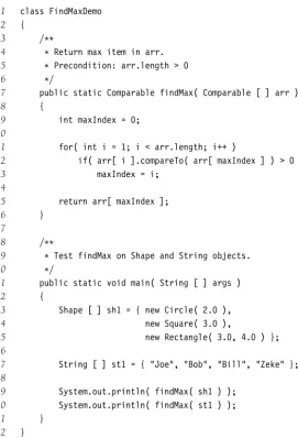
Consider, for example, the problem of finding the maximum item in an array of items. The basic code is type-independent, but it does require the ability to compare any two objects and decide which is larger and which is smaller. Thus we cannot simply find the maximum of an array ofObject—we need more information. The simplest idea would be to find the maximum of an array ofComparable. To determine order, we can use thecompareTo
method that we know must be available for allComparables. The code to do this is shown in Figure 1.8, which provides amainthat finds the maximum in an array ofStringorShape. It is important to mention a few caveats. First, only objects that implement the
Comparableinterface can be passed as elements of theComparablearray. Objects that have a
compareTomethod but do not declare that they implementComparableare notComparable, and do not have the requisiteIS-Arelationship. Thus, it is presumed thatShapeimplements
1 public class WrapperDemo
2 {
3 public static void main( String [ ] args )
4 {
5 MemoryCell m = new MemoryCell( );
6
7 m.write( new Integer( 37 ) );
8 Integer wrapperVal = (Integer) m.read( );
9 int val = wrapperVal.intValue( );
10 System.out.println( "Contents are: " + val );
11 }
12 }
1.4 Implementing Generic Components Pre-Java 5 15
1 class FindMaxDemo
2 {
3 /**
4 * Return max item in arr.
5 * Precondition: arr.length > 0
6 */
7 public static Comparable findMax( Comparable [ ] arr )
8 {
9 int maxIndex = 0;
10
11 for( int i = 1; i < arr.length; i++ )
12 if( arr[ i ].compareTo( arr[ maxIndex ] ) > 0 )
13 maxIndex = i;
14
15 return arr[ maxIndex ];
16 }
17
18 /**
19 * Test findMax on Shape and String objects.
20 */
21 public static void main( String [ ] args )
22 {
23 Shape [ ] sh1 = { new Circle( 2.0 ),
24 new Square( 3.0 ),
25 new Rectangle( 3.0, 4.0 ) };
26
27 String [ ] st1 = { "Joe", "Bob", "Bill", "Zeke" }; 28
29 System.out.println( findMax( sh1 ) );
30 System.out.println( findMax( st1 ) );
31 }
32 }
Figure 1.8 A genericfindMaxroutine, with demo using shapes and strings (pre-Java 5)
theComparable interface, perhaps comparing areas ofShapes. It is also implicit in the test program thatCircle,Square, andRectangleare subclasses ofShape.
Second, if theComparablearray were to have two objects that are incompatible (e.g., a
Stringand aShape), thecompareTomethod would throw aClassCastException. This is the expected (indeed, required) behavior.
Third, as before, primitives cannot be passed asComparables, but the wrappers work because they implement theComparableinterface.
Fourth, it is not required that the interface be a standard library interface.
16 Chapter 1 Introduction
while the interface is a user-defined interface. And if the class is final, we can’t extend it to create a new class. Section 1.6 offers another solution for this problem, which is the function object. The function object uses interfaces also and is perhaps one of the central themes encountered in the Java library.
1.4.4 Compatibility of Array Types
One of the difficulties in language design is how to handle inheritance for aggregate types. Suppose thatEmployeeIS-APerson. Does this imply thatEmployee[]IS-APerson[]? In other words, if a routine is written to acceptPerson[]as a parameter, can we pass anEmployee[]
as an argument?
At first glance, this seems like a no-brainer, andEmployee[]should be type-compatible withPerson[]. However, this issue is trickier than it seems. Suppose that in addition to
Employee,StudentIS-A Person. Suppose theEmployee[] is type-compatible withPerson[]. Then consider this sequence of assignments:
Person[] arr = new Employee[ 5 ]; // compiles: arrays are compatible arr[ 0 ] = new Student( ... ); // compiles: Student IS-A Person
Both assignments compile, yet arr[0] is actually referencing an Employee, and Student IS-NOT-A Employee. Thus we have type confusion. The runtime system cannot throw a
ClassCastExceptionsince there is no cast.
The easiest way to avoid this problem is to specify that the arrays are not type-compatible. However, in Java the arraysaretype-compatible. This is known as acovariant array type. Each array keeps track of the type of object it is allowed to store. If an incompatible type is inserted into the array, the Virtual Machine will throw an
ArrayStoreException.
The covariance of arrays was needed in earlier versions of Java because otherwise the calls on lines 29 and 30 in Figure 1.8 would not compile.
1.5 Implementing Generic Components
Using Java 5 Generics
1.5 Implementing Generic Components Using Java 5 Generics 17
1.5.1 Simple Generic Classes and Interfaces
Figure 1.9 shows a generic version of theMemoryCellclass previously depicted in Figure 1.5. Here, we have changed the name toGenericMemoryCellbecause neither class is in a package and thus the names cannot be the same.
When a generic class is specified, the class declaration includes one or more type parameters enclosed in angle brackets <> after the class name. Line 1 shows that the
GenericMemoryCelltakes one type parameter. In this instance, there are no explicit restric-tions on the type parameter, so the user can create types such asGenericMemoryCell<String>
andGenericMemoryCell<Integer>but not GenericMemoryCell<int>. Inside the GenericMemo-ryCellclass declaration, we can declare fields of the generic type and methods that use the generic type as a parameter or return type. For example, in line 5 of Figure 1.9, the
writemethod forGenericMemoryCell<String>requires a parameter of typeString. Passing anything else will generate a compiler error.
Interfaces can also be declared as generic. For example, prior to Java 5 theComparable
interface was not generic, and itscompareTo method took anObjectas the parameter. As a result, any reference variable passed to thecompareTo method would compile, even if the variable was not a sensible type, and only at runtime would the error be reported as aClassCastException. In Java 5, theComparableclass is generic, as shown in Figure 1.10. TheString class, for instance, now implementsComparable<String> and has a compareTo
method that takes aStringas a parameter. By making the class generic, many of the errors that were previously only reported at runtime become compile-time errors.
1 public class GenericMemoryCell<AnyType>
2 {
3 public AnyType read( )
4 { return storedValue; }
5 public void write( AnyType x )
6 { storedValue = x; }
7
8 private AnyType storedValue;
9 }
Figure 1.9 Generic implementation of theMemoryCellclass
1 package java.lang; 2
3 public interface Comparable<AnyType>
4 {
5 public int compareTo( AnyType other );
6 }
18 Chapter 1 Introduction
1.5.2 Autoboxing/Unboxing
The code in Figure 1.7 is annoying to write because using the wrapper class requires creation of anIntegerobject prior to the call towrite, and then the extraction of theint
value from theInteger, using theintValuemethod. Prior to Java 5, this is required because if anintis passed in a place where anIntegerobject is required, the compiler will generate an error message, and if the result of anIntegerobject is assigned to anint, the compiler will generate an error message. This resulting code in Figure 1.7 accurately reflects the distinction between primitive types and reference types, yet it does not cleanly express the programmer’s intent of storingints in the collection.
Java 5 rectifies this situation. If an int is passed in a place where an Integer is required, the compiler will insert a call to theIntegerconstructor behind the scenes. This is known as autoboxing. And if anIntegeris passed in a place where anintis required, the compiler will insert a call to theintValuemethod behind the scenes. This is known as auto-unboxing. Similar behavior occurs for the seven other primitive/wrapper pairs. Figure 1.11a illustrates the use of autoboxing and unboxing in Java 5. Note that the enti-ties referenced in theGenericMemoryCellare stillIntegerobjects;intcannot be substituted forIntegerin theGenericMemoryCellinstantiations.
1.5.3 The Diamond Operator
In Figure 1.11a, line 5 is annoying because sincemis of typeGenericMemoryCell<Integer>, it is obvious that object being created must also beGenericMemoryCell<Integer>; any other type parameter would generate a compiler error. Java 7 adds a new language feature, known as the diamond operator, that allows line 5 to be rewritten as
GenericMemoryCell<Integer> m = new GenericMemoryCell<>( );
The diamond operator simplifies the code, with no cost to the developer, and we use it throughout the text. Figure 1.11b shows the Java 7 version, incorporating the diamond operator.
1 class BoxingDemo
2 {
3 public static void main( String [ ] args )
4 {
5 GenericMemoryCell<Integer> m = new GenericMemoryCell<Integer>( ); 6
7 m.write( 37 );
8 int val = m.read( );
9 System.out.println( "Contents are: " + val );
10 }
11 }
1.5 Implementing Generic Components Using Java 5 Generics 19
1 class BoxingDemo
2 {
3 public static void main( String [ ] args )
4 {
5 GenericMemoryCell<Integer> m = new GenericMemoryCell<>( ); 6
7 m.write( 5 );
8 int val = m.read( );
9 System.out.println( "Contents are: " + val );
10 }
11 }
Figure 1.11b Autoboxing and unboxing (Java 7, using diamond operator)
1.5.4 Wildcards with Bounds
Figure 1.12 shows a static method that computes the total area in an array ofShapes (we assumeShapeis a class with anareamethod;CircleandSquareextendShape). Suppose we want to rewrite the method so that it works with a parameter that isCollection<Shape>.
Collectionis described in Chapter 3; for now, the only important thing about it is that it stores a collection of items that can be accessed with an enhanced forloop. Because of the enhancedforloop, the code should be identical, and the resulting code is shown in Figure 1.13. If we pass aCollection<Shape>, the code works. However, what happens if we pass aCollection<Square>? The answer depends on whether aCollection<Square>IS-A Collection<Shape>. Recall from Section 1.4.4 that the technical term for this is whether we have covariance.
In Java, as we mentioned in Section 1.4.4, arrays are covariant. So Square[] IS-A Shape[]. On the one hand, consistency would suggest that if arrays are covariant, then collections should be covariant too. On the other hand, as we saw in Section 1.4.4, the covariance of arrays leads to code that compiles but then generates a runtime exception (anArrayStoreException). Because the entire reason to have generics is to generate compiler
1 public static double totalArea( Shape [ ] arr )
2 {
3 double total = 0;
4
5 for( Shape s : arr )
6 if( s != null )
7 total += s.area( );
8
9 return total;
10 }
20 Chapter 1 Introduction
1 public static double totalArea( Collection<Shape> arr )
2 {
3 double total = 0;
4
5 for( Shape s : arr )
6 if( s != null )
7 total += s.area( );
8
9 return total;
10 }
Figure 1.13 totalAreamethod that does not work if passed aCollection<Square>
1 public static double totalArea( Collection<? extends Shape> arr )
2 {
3 double total = 0;
4
5 for( Shape s : arr )
6 if( s != null )
7 total += s.area( );
8
9 return total;
10 }
Figure 1.14 totalAreamethod revised with wildcards that works if passed a
Collection<Square>
errors rather than runtime exceptions for type mismatches, generic collections are not covariant. As a result, we cannot pass aCollection<Square>as a parameter to the method in Figure 1.13.
What we are left with is that generics (and the generic collections) are not covariant (which makes sense), but arrays are. Without additional syntax, users would tend to avoid collections because the lack of covariance makes the code less flexible.
Java 5 makes up for this with wildcards. Wildcards are used to express subclasses (or superclasses) of parameter types. Figure 1.14 illustrates the use of wildcards with a bound to write atotalAreamethod that takes as parameter aCollection<T>, whereTIS-A Shape. Thus,Collection<Shape> and Collection<Square> are both acceptable parameters. Wildcards can also be used without a bound (in which caseextends Objectis presumed) or withsuperinstead ofextends(to express superclass rather than subclass); there are also some other syntax uses that we do not discuss here.
1.5.5 Generic Static Methods
1.5 Implementing Generic Components Using Java 5 Generics 21
1 public static <AnyType> boolean contains( AnyType [ ] arr, AnyType x )
2 {
3 for( AnyType val : arr )
4 if( x.equals( val ) )
5 return true;
6
7 return false;
8 }
Figure 1.15 Generic static method to search an array
class declaration. Sometimes the specific type is important perhaps because one of the following reasons apply:
1. The type is used as the return type.
2. The type is used in more than one parameter type.
3. The type is used to declare a local variable.
If so, then an explicit generic method with type parameters must be declared.
For instance, Figure 1.15 illustrates a generic static method that performs a sequential search for valuexin arrayarr. By using a generic method instead of a nongeneric method that usesObjectas the parameter types, we can get compile-time errors if searching for an
Applein an array ofShapes.
The generic method looks much like the generic class in that the type parameter list uses the same syntax. The type parameters in a generic method precede the return type.
1.5.6 Type Bounds
Suppose we want to write afindMaxroutine. Consider the code in Figure 1.16. This code cannot work because the compiler cannot prove that the call tocompareToat line 6 is valid;
compareTois guaranteed to exist only ifAnyType isComparable. We can solve this problem
1 public static <AnyType> AnyType findMax( AnyType [ ] arr )
2 {
3 int maxIndex = 0;
4
5 for( int i = 1; i < arr.length; i++ )
6 if( arr[ i ].compareTo( arr[ maxIndex ] ) > 0 )
7 maxIndex = i;
8
9 return arr[ maxIndex ];
10 }
22 Chapter 1 Introduction
1 public static <AnyType extends Comparable<? super AnyType>> 2 AnyType findMax( AnyType [ ] arr )
3 {
4 int maxIndex = 0;
5
6 for( int i = 1; i < arr.length; i++ )
7 if( arr[ i ].compareTo( arr[ maxIndex ] ) > 0 )
8 maxIndex = i;
9
10 return arr[ maxIndex ]; 11 }
Figure 1.17 Generic static method to find largest element in an array. Illustrates a bounds on the type parameter
by using atype bound. The type bound is specified inside the angle brackets<>, and it specifies properties that the parameter types must have. A naïve attempt is to rewrite the signature as
public static <AnyType extends Comparable> ...
This is naïve because, as we know, theComparableinterface is now generic. Although this code would compile, a better attempt would be
public static <AnyType extends Comparable<AnyType>> ...
However, this attempt is not satisfactory. To see the problem, suppose Shape imple-mentsComparable<Shape>. SupposeSquareextendsShape. Then all we know is thatSquare
implements Comparable<Shape>. Thus, a Square IS-A Comparable<Shape>, but it IS-NOT-A Comparable<Square>!
As a result, what we need to say is thatAnyTypeIS-AComparable<T>whereTis a super-class ofAnyType. Since we do not need to know the exact typeT, we can use a wildcard. The resulting signature is
public static <AnyType extends Comparable<? super AnyType>>
Figure 1.17 shows the implementation of findMax. The compiler will accept arrays of types T only such that T implements the Comparable<S> interface, where T IS-A S. Certainly the bounds declaration looks like a mess. Fortunately, we won’t see anything more complicated than this idiom.
1.5.7 Type Erasure
1.5 Implementing Generic Components Using Java 5 Generics 23
to generic methods that have an erased return type, casts are inserted automatically. If a generic class is used without a type parameter, the raw class is used.
One important consequence of type erasure is that the generated code is not much different than the code that programmers have been writing before generics and in fact is not any faster. The significant benefit is that the programmer does not have to place casts in the code, and the compiler will do significant type checking.
1.5.8 Restrictions on Generics
There are numerous restrictions on generic types. Every one of the restrictions listed here is required because of type erasure.
Primitive Types
Primitive types cannot be used for a type parameter. ThusGenericMemoryCell<int>is illegal. You must use wrapper classes.
instanceof
tests
instanceoftests and typecasts work only with raw type. In the following code
GenericMemoryCell<Integer> cell1 = new GenericMemoryCell<>( ); cell1.write( 4 );
Object cell = cell1;
GenericMemoryCell<String> cell2 = (GenericMemoryCell<String>) cell; String s = cell2.read( );
the typecast succeeds at runtime since all types areGenericMemoryCell. Eventually, a run-time error results at the last line because the call toreadtries to return aStringbut cannot. As a result, the typecast will generate a warning, and a correspondinginstanceof test is illegal.
Static Contexts
In a generic class, static methods and fields cannot refer to the class’s type variables since, after erasure, there are no type variables. Further, since there is really only one raw class, static fields are shared among the class’s generic instantiations.
Instantiation of Generic Types
It is illegal to create an instance of a generic type. IfTis a type variable, the statement
T obj = new T( ); // Right-hand side is illegal
is illegal.Tis replaced by its bounds, which could beObject(or even an abstract class), so the call tonewcannot make sense.
Generic Array Objects
It is illegal to create an array of a generic type. IfTis a type variable, the statement
24 Chapter 1 Introduction
is illegal.Twould be replaced by its bounds, which would probably beObject, and then the cast (generated by type erasure) toT[]would fail becauseObject[]IS-NOT-AT[]. Because we cannot create arrays of generic objects, generally we must create an array of the erased type and then use a typecast. This typecast will generate a compiler warning about an unchecked type conversion.
Arrays of Parameterized Types
Instantiation of arrays of parameterized types is illegal. Consider the following code:
1 GenericMemoryCell<String> [ ] arr1 = new GenericMemoryCell<>[ 10 ];
2 GenericMemoryCell<Double> cell = new GenericMemoryCell<>( ); cell.write( 4.5 ); 3 Object [ ] arr2 = arr1;
4 arr2[ 0 ] = cell;
5 String s = arr1[ 0 ].read( );
Normally, we would expect that the assignment at line 4, which has the wrong type,