Geo-cognitive computing method for identifying “source-sink”
landscape
patterns of river basin non-point source pollution
Zhang Xin
1,
Cui Jintian
1,2*,
Liu Yuqi
1,2,
Wang Lei
3(1. State Key Laboratory of Remote Sensing Science, Institute of Remote Sensing and Digital Earth, Chinese Academy of Sciences, Beijing 100101, China; 2. University of Chinese Academy of Sciences, Beijing 100049, China; 3. Sanya Research Center,
Institute of Remote Sensing and Digital Earth, Chinese Academy of Sciences, Sanya 572029, Hainan Province, China)
Abstract: The aim of this study was to quantitatively evaluate the influences of landscape composition and spatial structure on the transmission process of non-point source pollutants in different regions. The location-weighted landscape contrast index, using the hydrological response unit (HRULCI) as the minimum research unit, was proposed in this paper. Through the description of the endemic landscape types and various geographical factors in the basin, the index calculation can reflect the impact of the “source-sink” landscape structure on the non-point source pollution in different regions and quantitatively evaluate the contribution of different landscape types and geographical factors to non-point source pollution. This study constructed a method of geo-cognitive computing for identifying “source-sink” landscape patterns of river basin non-point source pollution at two levels. 1) The basin level: the spatial distribution and landscape combination of the entire basin are identified, and the crucial “source” and “sink” landscape types are obtained to measure the differences in the non-point source pollutant transmission processes between the “source” and “sink” landscapes in the different watersheds. 2) The landscape level: HRULCI is calculated based on multiple geographical correction weighting factors. By using the idea of intersecting geographic information system (GIS) and landscape ecology, the landscape spatial pattern and ecological processes are linked. Compared with the traditional method for studying landscape patterns, the calculation of HRULCI makes the proposed method more ecologically significant. Lastly, a case study was evaluated to verify the significance of the proposed research method by taking the Yanshi River basin, a sub-basin belonging to the Jiulong River basin located in Fujian Province, China, as the experimental study zone. The results showed that this method can reflect the spatial distribution characteristics of the “source-sink” types and their relationship with non-point source pollution. By comparing the resulting calculation based on HRULCI, the risk of nutrient loss and the influence of landscape patterns and ecological processes on non-point pollution in different catchments can be obtained.
Keywords: non-point source pollution, “source-sink” landscape pattern, remote sensing, hydrological response unit, quantitative calculation
DOI: 10.25165/j.ijabe.20171005.3272
Citation: Zhang X, Cui J T, Liu Y Q, Wang L. Geo-cognitive computing method for identifying “source-sink” landscape patterns of river basin non-point source pollution. Int J Agric & Biol Eng, 2017; 10(5): 55–68.
1 Introduction
Water pollution is a major problem that restricts the sustainable development of China and the whole world,
Received date: 2017-02-21 Accepted date: 2017-09-10
Biographies: Zhang Xin, PhD, Researcher, research interests: spatial analysis and simulation, Email: [email protected];
Liu Yuqi, Master degree candidate, research interests: landscape spatial analysis, Email: [email protected]; Wang Lei, PhD, Associate Researcher, research interests: spatial analysis, Email:
and non-point source pollution is one of the most difficult problems to control. Since the 1960s, the research and treatment of non-point source pollution have been of great concern to the international environmental protection community. The United States Clean Water
Act Amendment of 1977 defined non-point source pollution as “Pollutants that enter the surface and groundwater in a wide, scattered, and micro form”. Because non-point source pollution is closely related to human activities and environmental conditions, such as atmosphere, hydrology, soil, vegetation, geology, geomorphology, and topography, and because it cannot be monitored in time and space, non-point source pollution is characterized by randomness, extensiveness, fuzziness, latency, and it is difficult to control[1]. At present, non-point source pollution has become a worldwide global environmental problem. According to statistics, 30%-50% of the earth’s surface has been affected by non-point source pollution[2]. In fact, 73% of biochemical oxygen demand (BOD), 92% of suspended matter and 83% of bacteria in US rivers are caused by non-point source pollution. Additionally, 89% of the annual nitrogen load in Mexico Bay comes from non-point source pollution, and water eutrophication is serious in Europe. The total nitrogen and total phosphorus produced in agricultural activities heavily imported into the Beihai Estuary account for 60% and 25% of the total nitrogen load and total phosphorus load, respectively. In Denmark and the Netherlands, 94% and 52%, respectively, of the total nitrogen load and 60% and 40%-50%, respectively, of the total phosphorus load contribute to agricultural non-point source pollution, representing the main sources of water quality pollution[3,4]. At present, some studies of the Songhua River, the Huaihe River, Taihu Lake, and Chaohu Lake in China have shown that at least 50% of the water pollution load is contributed by non-point sources[5]. Therefore, the severity of non-point source pollution has gradually emerged, and controlling non-point source pollution in a watershed has become a key task of water environment management.
The interaction between landscape patterns and ecological processes is an important part of landscape ecology research. Landscape pattern influences the process of pollutant transmission and affects the occurrence, migration and transformation of non-point source pollutants[6,7]. Therefore, exploring the hydrological response of landscape patterns has always
spatial allocation and this proportion of landscape area have certain impacts on pollution load. However, due to differences in land-use patterns and in the intensity of human activity, the non-point source pollution load that is produced and exported is very different in different types of landscapes[19]. Therefore, it is very difficult to simulate the space-time migration of non-point source pollution in complex landscapes. Most studies have analysed the influence of landscape pattern on river water quality by establishing the statistical relationship between pollution loads and land-use or runoff. Since the landscape pattern and ecological processes are related to different research scales and because they both change with scale[20], it is difficult to quantitatively describe the relationship between the landscape pattern and ecological processes in the present study. In view of this situation, this paper proposed a method of geo-cognitive computing for identifying “source-sink” patterns in the non-point pollution landscape of a river basin, this is significant in that it will enhance our knowledge of landscape patterns and watershed ecological processes.
Landscape characteristics have substantial effects on non-point source pollution[21]. The “source-sink” theory was derived from the fields of air pollution, biodiversity, etc. The concept of “source-sink” landscape theory is mainly based on the ecological balance theory of ecology. Some landscape types are sources of pollutants and thus play a “source” role, and some landscape types have the ability to reduce non-point source pollution and thus represent the “sink” type. The distance, relative height and slope of the landscape relative to the basin can influence the non-point source pollution in the basin[22]. Therefore, it is of great significance to measure non-point source pollution in watersheds by studying the type, distribution and function of the “source” and “sink” landscapes. Taking the basin as the study area, this paper analysed the spatial layout and function of different “source” and “sink” landscape types in order to quantify the contribution of various landscape types and ecological processes to the formation of non-point source pollution. Using the “source-sink” theory, this paper presented a method of geo-cognitive computing for identifying “source-sink” patterns of the non-point source pollution
landscape from two levels. 1) Basin level: The spatial distribution and landscape combination of the entire basin were identified, and the crucial “source” and “sink” landscape types were obtained to measure differences in the non-point source pollutant transmission processes between “source” and “sink” landscapes in different watersheds. 2) Landscape level: The hydrological response unit (HRU), with only a single land use and soil type, was used as the minimum calculated cell. Then, based on the hydrological response unit, the location-weighted landscape contrast index (HRULCI) was constructed. In this process, the weight of the emission of a certain pollutant from a “source” landscape type or a “sink” landscape type was calculated based on multiple geographical factors. Through the above steps, the landscape spatial pattern analysis was closely integrated with the ecological processes and thus quantitatively described the spatial distribution characteristics of the “source-sink” landscape types and their relationships with non-point source pollution. This approach enabled the systematic construction of the method of geo-cognitive computing for identifying “source-sink”landscape patterns of non-point pollution in a river basin. A case study was then carried out in the Yanshi River basin in Fujian Province.
2 Materials and methods
2.1 Research area and data sources
Longyan environmental monitoring station results of high-, normal-, and low-flow years in recent years, it was shown that the water quality of the Yanshi River basin has been seriously affected by pollution. Therefore, it is necessary to further clarify the spatial characteristics of watershed non-point source pollution in order to implement comprehensive prevention and control of the water environment in the river basin.
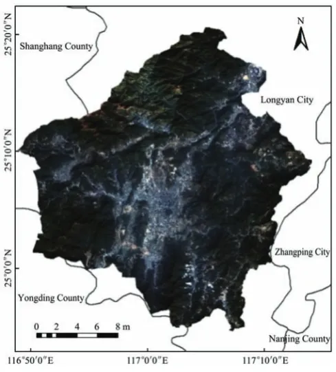
Figure 1 Remote sensing image from the Gaofen-2 satellite of the Yanshi River basin in 2014
Remote sensing technology expands the spatial capability of non-point source pollution research and compensates for the lack of ground monitoring technology[23,24]. Therefore, this paper applied remote sensing and GIS technology to study the non-point source pollution in the Yanshi River basin. The data used to build the geo-cognitive computing model for “source-sink” landscapepatterns of non-point pollution in the river basin include a GenFen-2 image from 2014, DEM (Digital Elevation Model) data of the Yanshi River basin with a 30-m spatial resolution, 1:1 million Chinese soil-type data, and precipitation data from the 2014 statistical yearbook of Fujian Province. Firstly, the GenFen-2 image was pre-processed (including geometric rectification, image registration and image fusion) to produce integrated satellite images of the Yanshi River basin. Secondly, the land-use classification of the study
area was obtained by visual interpretation using the Arc GIS 10.2 platform to produce a more accurate map of “source” and “sink” landscapes types. Thirdly, the DEM data were used to obtain slope data and the surface distance from the Yanshi River and catchment area. The soil types and available water content (AWC) of soil were obtained using the China 1:100 million soil database and the main soil types in the study area. The annual precipitation data were produced by spatial interpolation. 2.2 Landscape “source-sink” theory
“source-sink” landscapepatterns of non-point pollution in the river basin and comprehensively considered the effects of landscape patches and ecological processes on non-point source pollution.
2.3 Construction of the geo-cognitive computing model for the “source-sink” landscape patterns of non-point pollution in the river basin
The study in the Yanshi River basin was carried out based on the preceding “source-sink” theory and multidisciplinary theory and practice. Due to different catchment areas with special hydrologic properties, the catchment areas in the Yanshi River basin were divided, and the relationships between “source-sink” landscape patterns and non-point source pollution were evaluated in 24 catchment areas. The factors affecting the hydrological phenomena in the catchment area include geology, topography, meteorology (energy, precipitation, evaporation, evapotranspiration), soil, vegetation, and human activities. Therefore, it was very important to choose the appropriate evaluation unit for the quantitative study of the relationship between landscape pattern and non-point source pollution. A hydrological response unit (HRU) refers to a region in which the underlying surface is relatively uniform and homogeneous, and the
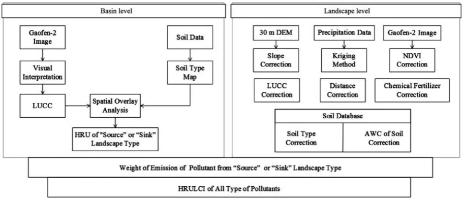
grids in this region have similar hydrological characteristics[25]. The method of HRU division can fully reflect both heterogeneity and similarity in the basin space. Theoretically, the hydrological response of landscape pattern based on a HRU scale is much higher than that based on the basin scale. Therefore, this study used a HRU as a minimum computational unit to analyse non-point source pollution in the basin. On this basis, this paper constructed the method of geo-cognitive computing for identifying “source-sink” patterns of the non-point source pollution landscape from two levels (Figure 2). Through the analysis of watershed level and landscape level, the landscape spatial pattern analysis was closely integrated with the ecological processes and thus quantitatively described the spatial distribution characteristics of the “source-sink” landscape types and their relationships with non-point source pollution. The index reflects the relative distribution of “source-sink” landscape types in space; the larger the index is, the greater the impact the basin (catchment area) has on the non-point source pollution process. Based on the above steps, the spatial distribution characteristics of the “source-sink” landscape types and their relationships with non-point source pollution are quantitatively described.
Figure 2 Research method flowchart
2.3.1 Catchment area division
The process of catchment area division was divided into five steps: DEM generation, flow direction setting, calculation of confluence accumulation, extraction of river network, and catchment area division. The Hydrology Model in Arc GIS version 10.2 provides an
by calculating the length error between the observed value and the calculated value of the starting point of flow direction to set a reasonable threshold.
1 1
( n ( )i m n ( ) ) /j m L
m m
R S S S
= =
=
∑
+∑
(1)where, Si is the insufficient water flow length, m; Sj is the
excessive water flow length, m; SL is the total length of the
river (m), which refers to the reach with insufficient or excessive water flow length; n refers to the total number of reaches with insufficient or excessive water flow length; R is the moderate index. The corresponding threshold is considered most reasonable when the value of R is small.
According to the geomorphological features of the study area, different catchment area thresholds were selected to extract the river network. Through the projection transformation and image registration, the processed images were superimposed on the remote sensing images of the same area. The starting point of the river was determined by Arc GIS10.2 software, and the excessive and insufficient water flow length of each image was calculated separately using Equation (1) to calculate the value of R. By performing function fitting for the value of R with the corresponding threshold, the threshold corresponding to the minimum R value was selected for subsequent processing. With the support of GIS and spatial analysis software and by using the DEM data and terrain features, the study area was divided into 24 catchment areas (Figure 3).
Figure 3 Catchment area division in the Yanshi River basin
2.3.2 Hydrological response unit division
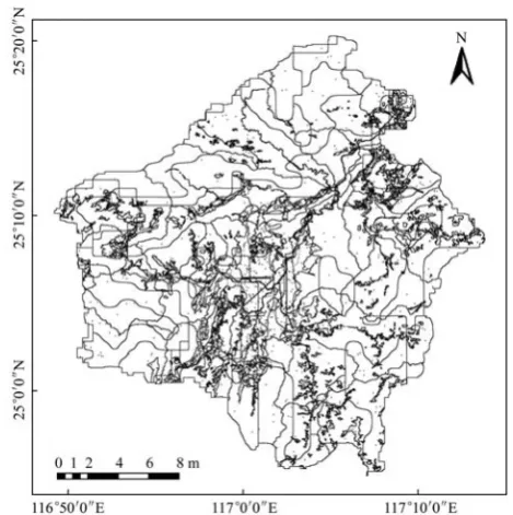
A hydrological response unit (HRU) refers to a region with the same land-use type and soil type, and the grids within this region have similar hydrological characteristics. The division of HRU can fully reflect the heterogeneity and similarity of the river basin. The process of HRU division is as follows. 1) Obtain the spatial distribution map of “source-sink” landscape types in the study area. The Gaofen-2 image was used to extract watershed landscape information, and land-use types were divided into two categories by artificial visual interpretation: “source” landscape types and “sink” landscape types. 2) Obtain soil type map. Soil information was obtained from the 1:100 million Chinese soil texture data. According to the actual situation of the study area, the main soil types were obtained and included red soil, paddy soil, purple soil, and yellow soil. 3) Determine hydrological response unit division. The spatial overlay was made using the catchment area map, the “source-sink” landscape type spatial distribution map and the soil type map so that each HRU only has a single land-use type and soil type. The result of the hydrological response unit division was obtained by the method described above (Figure 4).
Figure 4 Hydrological response unit division in the Yanshi River basin
2.3.3 Geographical factors and correction coefficient calculation
different roles in the process of non-point source pollution formation, the distance, relative height and slope of the landscape relative to the basin can influence the non-point source pollution in the basin. In addition, the transmission and migration of non-point source pollutants are affected by factors such as rainfall, soil type, available water content of soil, vegetation distribution, and fertilizer application. Considering the influence of geographical factors on non-point source pollution transmission in the basin, land-use and land-cover change (LUCC), slope, precipitation, effective distance, normalized difference vegetation index (NDVI), soil type, chemical fertilizer, and available water capacity (AWC) of soil were selected as influencing factors and used to quantitatively describe the contribution of different landscape types and geographical factors to non-point source pollution. The factors have two functions: the relationships between “source-sink” landscape types and ecological processes and non-point source pollution are intuitively described, and the factors are used to obtain the emission weight of a certain pollutant from a “source” landscape type or a “sink” landscape type to quantitatively evaluate how different landscape composition and spatial structure affect the transmission process of non-point source pollutants in different regions. With reference to the Chinese standard for the discharge coefficient of farmland runoff pollutants and the actual situation of the study area in 2014, we revised the influencing factors.
1) LUCC correction: Land use is the most direct form of human activity. Land cover change is closely related to the evolution of the natural environment and increasing human activities[27]. Inappropriate land-use activities and land management patterns lead to soil erosion and the loss of nutrients, resulting in large areas of non-point source pollution in the basin. In fact, the contribution of different landscape types to soil erosion and nutrient loss is quite different. Generally, cultivated land, orchard and urban construction land are the main areas of non-point source pollutants, while forest land, shrub land and grassland can intercept the nutrients or non-point source pollutants. For non-point source pollution, the contribution of “source” landscapes to non-point source pollution is mainly related to the use of pesticides and
fertilizers. Therefore, cultivated land is used as the reference landscape type. According to the consumption of pesticides, fertilizers and other sources of pollution, the weights of different “source” landscape types are determined. For the “sink” landscape type, forest land is used as the reference landscape type. The weights of different “sink” landscape types are determined based on their role in intercepting non-point source pollution. Therefore, the correction coefficient of cultivated land was approximately 1.7, the correction coefficient of orchards was 1.5, and the correction coefficient of industrial land and residential land was approximately 1.3. The correction coefficient of forest land and shrub land was approximately 0.7, the correction coefficient of wetland was 0.9, the correction coefficient of river and lake was approximately 0.5, and the correction coefficient of unused land was 0.3.
2) Slope correction: When the slope of the land is below 25°, the nutrient loss coefficient is 1.0-1.2; when the slope is greater than 25°, the nutrient loss coefficient is 1.2-1.5.
3) Precipitation correction: The correction coefficient of annual precipitation below 400 mL is 0.6-1.0, the correction coefficient of annual precipitation between 400 mL and 800 mL is 1.0-1.2, and the correction coefficient of annual precipitation above 800 mL is 1.2-1.5.
4) Effective distance correction: The closer the “source” landscape type is to the monitoring site, the greater the influence the “source” landscape has on the monitoring site. Conversely, its contribution to the monitoring site is smaller. However, the effect of a “sink” landscape on non-point source pollution is opposite of the effect of a “source” landscape.
Thus, the greater the NDVI value is, the greater the vegetation coverage.
NDVI NIR R NIR R
− =
+ (2)
where, NIR is the reflectance value near the infrared band and R is the reflectance value at the red band.
6) Soil type correction: The soil of the study area is divided according to the soil composition into sandy soil, loam and clay. The correction coefficient of loam is 1, the correction coefficient of sandy soil is 0.8-1.0, and the correction coefficient of clay is 0.6-0.8.
7) Chemical fertilizer correction: The value of the chemical fertilizer correction coefficient is determined according to the amount of fertilizer applied. If the amount of chemical fertilizer per mu is below 25 kg, the correction coefficient is 0.8-1.0; if the amount of chemical fertilizer per mu is between 25 kg and 35 kg, the correction coefficient is 1.0-1.2; and if the amount of chemical fertilizer per hectare is more than 2.3 kg, the correction coefficient is 1.2-1.5.
8) Available water content (AWC) of soil correction: The available water content of soil directly affects vegetation growth, soil nutrient migration and transformation, soil erosion and hydrological processes[28,29]. The soil suction is related to the available soil water content, which can be used as a driving force for water movement in the soil profile[30]. Smaller soil suction occurs in areas with higher soil water content, while soil water content decreases with sharply increasing soil suction.
2.3.4 Construction of the HRULCI
Different “source” and “sink” landscape types are different in the extent they discharge, absorb, or intercept non-point source pollution. Considering the influence of geographical factors in the process of non-point source pollution transmission in the watershed, the HRULCI is constructed to quantitatively evaluate the different effects “source” and “sink” landscape types and ecological processes may have on non-point source pollution. The HRULCI has a relatively comparative significance, the calculation result based on the HRULCI is larger, the contribution of the landscape spatial pattern and of the ecological processes on non-point source pollution in the
watershed (catchment area) is greater, and the risk of nutrient loss is greater. Conversely, the smaller the contribution. By comparing the HRULCI values of different catchment areas, it is possible to estimate the risk of non-point source pollution in the basin.
According to “source-sink” theory and catchment area division, the calculation equation of location-weighted landscape contrast index (HRULCI) is expressed as:
HRULCIi=Wi×Ai (3)
where, i is a special HRUi; Ai is the area of HRUi; Wi is the
emission weight of a certain pollutant from a “source” landscape type or a “sink” landscape type; Wi represents
the influence of various geographical factors in the transmission of non-point source pollution in the watershed.
The “source” and “sink” landscape types play different roles in the formation of non-point source pollution, and the influence of “source-sink” landscape pattern on non-point source pollution is mainly reflected by the slope, distance, height of the landscape relative to the monitoring site, vegetation distribution, precipitation process and other factors. In turn, these factors affect the spread of pollutants as well as interception, absorption and transformation. Therefore, this paper selected land-use and land-cover change (LUCC) correction, slope correction, precipitation correction, effective distance correction, normalized difference vegetation index (NDVI) correction, soil type correction, chemical fertilizer correction, and available water capacity (AWC) of soil correction as the non-point source pollutant correction weighting factors to calculate the value of weight Wi. Wi is expressed as:
Wi=F L P R D N S F A( , , , , , , , ) (4)
where, L is the LUCC correction; P is the slope correction; R is the precipitation correction; D is the effective distance correction; N is the NDVI correction; S is the soil type correction; F is the chemical fertilizer amendment correction; and A is the AWC of soil correction.
max i
W W
W
= (5)
where, Wi is a non-point source pollutant correction
weighting factor for the watershed landscape pattern; Wmax is the maximum value of the non-point source pollutant correction coefficient in the watershed landscape pattern.
During the formation of non-point source pollution, some landscape types play the role of “source” and can promote the transmission of non-point source pollution, while other landscape types play the role of “sink” and prevent and inhibit non-point source pollution. Therefore, according to the “source-sink” theory, the differences between the “source” and “sink” landscape types and ecological conditions in different catchment areas can be measured by the following equation:
1 1
n n
x ix i jx j
i j
CALCI W A W A
= =
=
∑
× −∑
× (6)where, CALCIx is the sum of HRULCIx in a catchment
area, and it represents the contribution of catchment area to pollutant X; i is a special HRUi of a “source” landscape;
j is a special HRUj of a “sink” landscape; Ai is the area of
HRUi; Aj is the area of HRUj; Wix is the emission weight
of pollutant X from a certain “source” landscape type; Wjx
is the weight of pollutant X that a certain “sink” landscape type accepts. Since the area of each catchment is different, in order to compare the calculation results of different catchment areas, any differences caused by the catchment areas are eliminated with the following equation:
/ x x CA
R =CALCI S (7)
where, SCA is the area of each catchment.
Considering the existence of various types of pollutants, CALCI can be expressed as:
xy x y
R =R +R (8)
where, x and y refer to different pollutants within the study.
When comparing the Rxy between different catchment
areas, the larger the value is, the greater contribution the landscape spatial pattern and ecological processes have on the non-point source pollution in the basin, and thus, the stronger the non-point source pollution effect.
3 Results
3.1 “Source” and “sink” classification
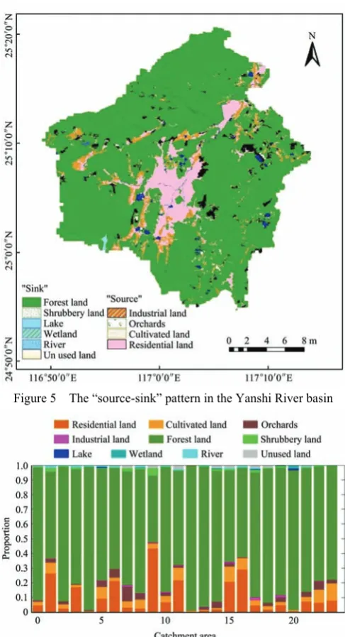
The “source” and “sink” landscape types in the Gaofen-2 image were classified by visual interpretation using ENVI 5.2 (Figure 5). The “source” landscape types included cultivated land, orchard, industrial land and residential land, and the “sink” landscape types included forest land, shrub land, lake, wetland, river and unused land. With the help of the MATLAB R2014a platform, the proportion of each land-use type in each catchment area was calculated. Then, the proportion histogram of “source” and “sink” landscape types in each catchment area was obtained. Figure 6 shows the area composition of the “source-sink” landscape types for each catchment.
Figure 5 The “source-sink” pattern in the Yanshi River basin
By analysing the results shown in Figure 6, the No. 9, 16, 1, 11, 6, and 15 catchment areas have a greater proportion of residential area. The No. 23, 15, 22, 11, 5, and 16 catchment areas have a greater proportion of cultivated land area. The No. 7, 6, 22, 8, 5, and 14 catchment areas have a greater proportion of orchard area, and the No. 23, 15, 22, 11, 5, and 16 catchment areas have a greater proportion of industrial land area. Due to the forest land of the Yanshi River basin accounting for more, forest and shrub lands are analysed as the main “sink” landscape types. It can be concluded that the No. 12, 4, 13, 20, 2, and 18 catchment areas have a greater proportion of forest area. The proportion of shrub land area, in decreasing order, is as follows: catchment area No. 9, 1, 7, 17, 14, and 19.
3.2 Realizing process of geographical correction factors
The eight geographical correction factors listed above were processed separately. The input data for
slope correction was extracted from DEM data in the study area using Arc GIS 10.2 (Figure 7a). The precipitation distribution in the study area was obtained using the Kriging interpolation method as was used as the input data for the precipitation correction. For effective distance, Arc GIS 10.2 was used to calculate the distance from the water body (Figure 7b) and to define the 20-km maximum for local water source protection as the most effective surface distance. The NDVI in the study area was calculated by ENVI 5.3 (Figure 7c). The soil type and available water content of soil were extracted from the China 1:100 million soil database. For the chemical fertilizer correction, information from the statistical yearbook of Fujian Province indicated that in 2014, the amount of chemical fertilizer used on cultivated land and orchards was approximately 16 693 kg/hm2. Therefore, the correction coefficient of cultivated land and orchard was 1.4, and that of other surface types was 0.8.
a. Slope b. Distance c. NDVI
Figure 7 Slope, distance and NDVI in the Yanshi River basin 3.3 Calculation results of the R value
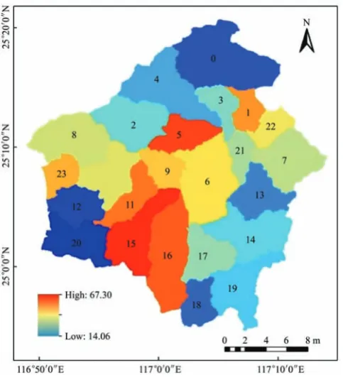
By analysing the quantitative results of the non-point source pollutant transmission process in different ecological conditions and “source-sink” landscape patterns within the catchment areas (Figure 8), it can be concluded that the calculated results of the R value within catchment areas 15, 5, 16, 11, 1, 23, and 9 were higher. Analysing the “source-sink” landscape patterns in these areas revealed that the area of cultivated land, residential and other “source” landscape types were relatively high. Compared with the natural landscape, artificial
and underground leakage and result in water pollution. The R values in catchment areas 6, 22, 10, and 8 were calculated. The “source” landscape types in these regions have large areas of orchards and residential land. Compared with cultivated land, the soil in orchard land is harder, and the soil and water conservation capacity is higher, leading to relatively low values of R. In addition, the “sink” landscape types in these regions were more abundant, which greatly weakens the transmission process of non-point source pollutants. The areas with low R values are mainly distributed in catchment areas 20, 0, 12, 13, 18 and 4. Additionally, the vegetation coverage in these areas is higher, and the forest, shrub, and wetland landscape types are widely distributed. Vegetation forms physical and biogeochemical barriers, increasing rainfall infiltration and reducing peak discharge, surface runoff velocity and sediment carrying capacity. On one hand, vegetation can reduce the generation of non-point source pollutants, but on the other hand, the pollutants carried by the water flow are intercepted, absorbed and transformed into harmless substances during migration. Thereby, the resilience of the ecosystem and the internal material circulation is enhanced, which greatly reduces harm caused by non-point source pollution.
Figure 8 The R value of each catchment area in the Yanshi River basin
From the perspective of spatial distribution, the R value of the central region of the Yanshi River basin is higher, likely because the area is very disturbed by human activities and other external factors, and the vegetation density in the area is relatively small. However, the R value is lower on the peripheral part of the central region.
The quantitative calculation results were graded by the natural breaks (Jenks) provided by Arc GIS: 14.06≤R1<28.26, 28.26≤R2<45.17, and 45.17≤R3<67.30 (Table 1). The
R
value represents the influence of landscape spatial pattern and ecological processes on the non-point source pollution in the basin. It can be concluded that the highest proportion was in the R2 range, accounting for 40.81% of the total basin area. The R1 range was second, accounting for 33.52%, and the R3 range accounted for 25.67%. The results showed that the current “source-sink” landscape pattern is good in the Yanshi River basin, and the negative effects of the ecological processes and geographical factors on the non-point source pollution process are not very significant; however, some areas with high R values still need to strengthen their management of non-point source pollution.Table 1 The proportion of R values in different grades
R R1 R2 R3
Proportion 33.52% 40.81% 25.67%
4 Discussion
The “source-sink” theory provides a new approach for studying non-point source pollution in the basin. In this paper, by analysing the spatial distribution of different “source” and “sink” landscape types as well as the effects of ecological factors on the formation and transmission of non-point source pollution, the location-weighted landscape contrast index based on the minimum hydrological response unit (HRULCI) was constructed to quantitatively evaluate the contribution of different landscape types and geographical factors to non-point source pollution in different catchment areas. The method has the following characteristics:
hydrological response unit and used to evaluate the non-point source pollution process in different catchment areas. In future studies, the method can be extended to larger research areas or applied to different small basins.
2) The non-point source pollution is affected by many factors, and the mechanisms of pollutant formation, transformation and migration are complicated. Therefore, this paper considered the influence of multiple geographical factors on the transmission of non-point source pollutants, thus avoiding the incomplete evaluation of the process by a single factor. In addition, the HRULCI reflects the relative spatial distributions of “source” and “sink” landscape types. In general, this method has important reference value in future evaluations of non-point source pollution risk, and the results can be used for regional landscape ecological planning.
3) The correlation between the spatial distribution of landscape patterns and the river water quality is very significant. Therefore, the non-point source pollution process is also influenced by the combination of the “source-sink” landscape pattern and spatial structure. According to the characteristics of different developing areas (rural areas, urban areas, etc.), the spatial distribution pattern of “source” and “sink” landscape types can be regulated and planned in areas with serious non-point source pollution using the quantitative calculation method proposed in this paper. For some heavily polluted areas, the reduction of “source” landscape types may control the movement of nutrients, increase the proportion of “sink” landscape types and improve the stability of fixed nutrients, ultimately promoting a more rational layout of “source” and “sink” landscapes.
5 Conclusions
The “source” and “sink” landscape is the transformation route for non-point source pollutants, and a change in the “source-sink” landscape pattern will affect the occurrence, migration and transformation of non-point source pollutants. The aim of this study was to quantitatively evaluate the influence of landscape
Acknowledgements
The authors would like to thank the anonymous reviewers for their constructive comments and suggestions. The study was funded by the National Key R&D Programs of China (Grant No. 2017YFB0504201, 2015BAJ02B02), the Natural Science Foundation of China (Grant No. 61473286, 61375002) and the Natural Science Foundation of Hainan Province (Grant No. 20164178).
[References]
[1] Munafò M, Cecchi G, Baiocco F, Mancini L. River pollution from non-point sources: a new simplified method of assessment. Journal of Environmental Management, 2005; 77: 93–98.
[2] Corwin D L, Vaughan P J, Loague K. Modeling non-point source pollutants in the vadose zone using GIS. Environmental Science and Technology, 1997; 31(8): 2157–2175.
[3] United States Environmental Protection Agency. National Water Quality Inventory, USA: 1998 Report to Congress, 2000.
[4] Boers P C M. Nutrient emissions from agriculture in the Netherlands, causes and remedies. Water Science and Technology, 1996; 4-5: 183–189.
[5] Cheng H F, Hu Y A, Zhao J F. Meeting China’s water shortage crisis: Current practices and challenges. Environmental Science and Technology, 2009; 43: 240–244. [6] Liu S L, Fu B J. Application of landscape ecology principle
in soil science. The Journal of Soil and Water Conservation, 2001; 15(3): 102–106.
[7] Verburg P H, Steeg J V D, Veldkamp A, Willemen L. From land cover change to land function dynamics: a major challenge to improve land characterization. Journal of Environmental Management, 2009; 90(3): 1327–1335. [8] Kibena J, Nhapi I, Gumindoga W. Assessing the
relationship between water quality parameters and changes in landuse patterns in the Upper Manyame River, Zimbabwe. Physics and Chemistry of the Earth, 2014; 67-69: 153–163. [9] Rajaei F, Sari A E, Salmanmahiny A, Delavar M, Bavani A
R M, Srinivasan R. Surface drainage nitrate loading estimate from agriculture fields and its relationship with landscape metrics in Tajan watershed. Paddy and Water Environment, 2017; 15(3): 541–552.
[10] Liess A, Le Gros A, Wagenhoff A, Townsend C R, Matthaei C D. Landuse intensity in stream catchments affects the benthic food web: consequences for nutrient supply, periphyton C:nutrient ratios, and invertebrate richness and
abundance. Freshwater Science, 2012; 31(3): 813–824. [11] Derek R. Implementing landscape indices to predict stream
water quality in an agricultural setting: an assessment of the Lake and River Enhancement (LARE) protocol in the Mississinewa River watershed, East-Central Indiana. Ecological Indicators, 2010; 10: 1102–1110.
[12] Chen L D, Fu B J, Xu J Y, Gong J. Location-weighted landscape contrast index: a scale independent approach for landscape pattern evaluation based on “Source-Sink” ecological processes. Acta Ecologica Sinica, 2003; 23(11): 2406–2413. (in Chinese)
[13] Wang J L, Shao J A, Wang D, Ni J P, Xie D T. Identification of the “source” and “sink” patterns influencing non-point source pollution in the Three Gorges Reservoir Area. Journal of Geographical Sciences, 2016; 10: 1431–1448.
[14] Bhaduri B, Harbor J, Engel B, Grove M. Assessing watershed-scale, long-term hydrologic impacts of land use change using a GIS-NPS model. Environment Management, 2000; 26(6): 643–658.
[15] Li Z, Liu W Z, Zhang X C, Zheng F L. Impacts of land use change and climate variability on hydrology in an agricultural catchment on the Loess Plateau of China. Journal of Hydrology, 2009; 377: 35–42.
[16] Merz R, Blǒschl G, Parajka J. Spatio-temporal variability of event runoff coefficients. Journal of Hydrology, 2006; 331: 591–604.
[17] Gergel S E.Spatial and non-spatial factors: When do they affect landscape indicators of watershed loading? Landscape Ecology, 2005; 20: 177–189.
[18] Moreno J L, Navarro C, Heras J D L. Abiotic ecotypes in south-central Spanish rivers: Reference conditions and pollution.Environmental Pollution, 2006; 143: 388–396. [19] Basnyat P, Teeter L D, Flynn K M, Lockaby B G.
Relationships between landscape characteristics and non-point source pollution inputs to coastal estuary. Environmental Management, 1999; 23(4): 539–549.
[20] Wu J G. Paradigm shift in ecology: an overview. Acta Ecologica Sinica, 1996; 16(5): 449–460.
[21] Shen Z Y, Hou X S, Li W, Aini G. Relating landscape characteristics to non-point source pollution in a typical urbanized watershed in the municipality of Beijing. Landscape and Urban Planning, 2014; 123: 96–107.
[22] Chen L D, Tian H Y, Fu B J, Zhao X F. Development of a new index for integrating landscape patterns with ecological processes at watershed scale. Chinese Geographical Science, 2009; 19: 37–45.
[24] Tim U S. Coupling vadose zone models with GIS: Emerging trends and potential bottlenecks. Journal of Environmental Quality, 1996; 25(3): 535–544.
[25] Ning J C, Gao Z Q, Lu Q S. Runoff simulation using a modified SWAT model with spatially continuous HRUs. Environmental Earth Sciences, 2015; 7: 5895–5905.
[26] Lin W-T, Chou W-C, Lin C-Y, Huang P-H, Tsai J-S. Automated suitable drainage network extraction from digital elevation models in Taiwan’s upstream watersheds. Hydro Process, 2006; 20(2): 289–306.
[27] Guo X D, Chen L D, Fu B J. Effects of land use / land cover changes on regional ecological environment. Chinese Journal of Environmental Engineering, 1999; 7(6): 66–75. (in
Chinese)
[28] Ersahin S, Brohi A R. Spatial variation of soil water content in topsoil and subsoil of a Typic Ustifluvent. Agricultural Water Management, 2006; 83(1-2): 79–86. [29] Western A W, Zhou S L, Grayson R B, McMahon T A,
Bloöschl G, Wilson D. Spatial correlation of soil moisture in small catchments and its relationship to dominant spatial hydrological processes. Journal of Hydrology, 2004; 286(1): 113–134.