Optimal design of velocity sensor for open channel flow using
CFD
Joseph Scot Dvorak
1*,
Naiqian Zhang
2(1. Department of Biosystems and Agricultural Engineering, University of Kentucky, Lexington, Kentucky 40546-0276, USA; 2. Department of Biological and Agricultural Engineering, Kansas State University, Manhattan, Kansas 66506, USA)
Abstract: In this study, computational fluid dynamics (CFD) was used to design the geometry of a new velocity sensor for
measuring open channel flows. This sensor determined velocity by observing the travel of dye carried in the flow. Evaluation of this design required the development of fluid dynamics models to determine potential errors in fluid velocity measurement due to velocity changes caused by intrusion of the sensor in the fluid. It also required an analysis technique to determine the expected sensor response to the flow fields that resulted from the CFD modeling. These models were then used to improve the geometry of the sensor to minimize the measurement error. Starting with a simple design for the sensor geometry, the CFD analysis modeled the open channel flow around the sensor as turbulent using both the k-ω and k-ε Reynolds Averaged Navier-Stokes (RANS) turbulence models. The model predicted that the original sensor design would underestimate the free-stream velocities of open channels by 7.9% to 2.0% across a range from 0.1 m/s to 5.0 m/s. After using CFD to improve the sensor design, the velocity measurement error was limited to less than 4% across the same velocity range.
Keywords: computational fluid dynamics, flow measurement, sensors, flow velocity, open channel DOI: 10.3965/j.ijabe.20171003.2147
Citation: Dvorak J S, Zhang N Q. Optimal design of velocity sensor for open channel flow using CFD. Int J Agric & Biol
Eng, 2017; 10(3): 130–142.
1 Introduction
For contact type open channel water velocity sensors, loading effect is always a major concern. When the sensor is placed within the fluid, it changes the local fluid velocities, thus yielding measurement errors. With traditional mechanical anemometer flow meters, careful and frequent calibration is required to account for this
Received date: 2015-09-23 Accepted date: 2016-12-08 Biographies: Naiqian Zhang, Professor, research interests:
automatic tractor and engine control, machine vision applications on precision agriculture, optical sensors, dielectric sensors, precision agriculture technologies, wireless sensor network, embedded systems, and plant phenotyping, Email: [email protected].
*Corresponding author: Joseph Scot Dvorak, Assistant Professor, research interests: agricultural machinery automation, hybrid and alternative energy drivetrains, sensors, machinery management and route optimization. Department of Biosystems and Agricultural Engineering, University of Kentucky, 128 C.E. Barnhart Building, Lexington, KY 40546-0276, USA. Tel: +1-859-257- 5658, Email: [email protected].
effect[1]. More recently developed sensor technologies
like acoustic Doppler velocimeters rely on non-contact techniques[2], and the fact that the velocity measuring point is not directly in contact with the sensor rather than calibration to adjust for the loading effect[3]. However, the sensors must still be in contact with the flow at some point. To address concerns about loading effects, the flow around the sensor body for any flow velocity sensor needs to be analyzed using tools such as computational fluid dynamics (CFD). After analyzing the design, improvements can be made to the sensor geometry to reduce the loading error.
Environmental sensors are becoming more ubiquitous and researchers are developing new sensors and methods to use this information in ever more powerful ways[5,6].
They can serve vital roles in aquaculture systems to monitor water quality and maintain optimal productivity[7], to monitor marine shellfish[8], and to manage nitrogen pollution[9]. This increased influence and impact makes it vital to consider geometry in design of open channel sensors. The complex geometry of many sensors and the complexity of natural flow systems frequently make traditional fluid flow analysis techniques impractical, and most designs must be based on simplifications and intuition. New tools like CFD and the analysis performed in this project enable a more thorough investigation of flows around these sensors.
Several researchers have used CFD in evaluating sensors built to monitor fluid flow. Mueller and colleagues[10] described using CFD to evaluate the effect of an acoustic Doppler profiler on the velocity of the fluid flow passing the probe. They used the renormalized group turbulence model, a refinement of the k-ε Reynolds Averaged Navier Stokes (RANS) model in their study. In addition to simulating the effect using CFD, they tested the system in the laboratory using particle image velocimetry. Through comparison, they found that the CFD simulations, while not perfect, were reasonable for use in evaluating the effect the sensor had on fluid flow velocity. In another study, Tokyay et al.[11] utilized Large Eddy Simulations (LES) to determine the flow disturbances caused by an acoustic Doppler current profiler mounted on a boat. They were able to determine that the sensor itself had an effect on the measured velocity. When comparing the laboratory measurements with simple RANS-based CFD models, they concluded that CFD modeling provided significant benefits for fluid flow studies around sensors.
The sensor designed in this project is a correlation-based optical flow velocity sensor. While ultrasonic-based sensors are commonly used for open-channel flow measurements, their sensing elements are expensive and susceptible to damage when mounted in streams[12], which is not the case for the robust LEDs
and phototransistors used in this sensor’s design. In addition, this sensor has been designed to provide
information on soil sediment concentration[13] as well as
velocity measurements. The basics of this sensor’s operation have been described by Zhang et al.[14] in more
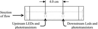
detail. The initial sensor design is shown in Figure 1. The sensor body was made of solid plastic material, into which were mounted two sets of LEDs and phototransistors—labeled upstream and downstream in Figure 1a. Within each set, light emitted by an LED was detected by two corresponding phototransistors. The LEDs and phototransistors in each set were located around a channel through the sensor and arranged as shown in Figure 1b. To measure velocity, a small amount of dye was released in the water upstream from the sensor, and the water carried the dye through the sensor. The dye first affected the signals from the upstream and then those from the downstream phototransistors. The sensor determined velocity by the time difference between the effects of the dye on the upstream and downstream phototransistors. This time difference was calculated using cross covariance. This same basic structure has proven useful in determining flow rates through sprayer nozzles[15] and with different calculation methods and calibrations for determining chemical concentrations in fluid flows[16].
a. Side view showing the two sets of LEDs and phototransistors
b. End view showing the placements of LED and phototransistors within each set
c. Three-dimensional view of the initial sensor design
d. Three-dimensional view of the initial sensor with an extension for dye injection
Figure 1 Internal structure of sensor
The extension of the sensor ensured detection of dye, but further improvements had to be made as the original electronics were designed for low power operation for other parts of the sensor system. Because of limited memory and processing speed, the electronics on the original sensor could only perform the cross covariance calculation which is used to determine velocity once every few minutes. Even then, the electronic limitations required a tradeoff between resolution of the velocity estimate or range over which the sensor could estimate velocity. Because of these velocity measurement limitations, the sensor was redesigned. As the electronics were improved to permit the velocity calculation within seconds, the physical geometry of the sensor was investigated to determine what effect it might
have on the measured velocity and how it could be improved. For this reason, the CFD analysis described here was carried out.
This sensor is intended to be installed in creeks for long periods of time to provide information about the flow velocity conditions. Therefore, it is expected that the sensor will be installed in relatively stable flow regions that reflect the general conditions in the entire creek. For this purpose, the sensor will be installed completely beneath the surface of the water and away from the bed or any wall where a particular geometry would have a significant boundary effect on the result. With this assumption, the analysis did not have to consider approximations for the free surface of the water or a myriad of different geometries for the streambed.
The objectives of this study were:
1) To simulate flow velocity changes due to intrusion of a physical fluid velocity sensor into an open channel and estimate the velocity measurement error within the free-stream water velocity range of 0.1 m/s to 5.0 m/s using the CFD method.
2) To develop a method to predict the velocity sensor readings based on the CFD results and to identify fluid flow features that are impacting the sensor readings.
3) To produce a final design of the sensor that would minimize the velocity measurement error to ±4% within the 0.1 m/s to 5.0 m/s velocity range.
2 Methods
2.1 CFD problem definition
the rear of the sensor. This resulted in a test volume that was a rectangular box or cuboid with dimensions of 400 mm plus the sensor’s width, 400 mm plus the sensor’s height, and 1 m plus the sensor’s length, which made the sensor a small part of a much larger flow.
When installed in the field, the sensor was supported through a connection point on the top of the sensor. Preliminary simulations included the bolts, nuts and brackets that provided the support hardware, but these items all mounted on the top of sensor toward the rear had no effect on the velocities through the flow detection channel in the sensor. The complexities of these multiple small hardware parts were removed because they significantly increased CFD processing time, and did not provide any additional benefit to the results.
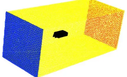
Figure 2 shows the sensor and the volume around the sensor used in the CFD analysis. In this figure, the face of the box upstream from the sensor is blue, the sides of the box are yellow, the sensor is black and the downstream face is red. The boundaries of this volume were defined to simulate the conditions of the sensor when it was installed in a stable part of a stream, away from the side, bed or surface of the stream. The surface of the sensor was modeled as a stationary, no-slip wall. The sides of the volume (highlighted in yellow in Figure 2) were defined as a symmetric boundary with zero normal velocity across the boundary and zero gradients for all properties at the boundary. The downstream face was set to allow the outflow of the fluid. The upstream face of the volume was set as the fluid inlet with a constant velocity normal to the boundary. Different free-stream velocities could be tested by varying the velocity setting at the inlet.
Figure 2 Sensor and volume around the sensor used for CFD analysis
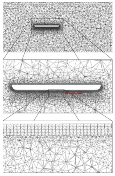
The geometry was modeled using two different computer programs. The geometry of the sensor body itself was modeled in the CAD program of Solid Works developed by Dassault Systèmes SolidWorks Corp (Waltham, Massachusetts). The resulting 3D representation of the sensor geometry was then exported as an STL file and imported into TGrid (version 13.0.0) by ANSYS (Canonsburg, Pennsylvania). TGrid was used to define the geometry around the sensor, the boundary conditions of that volume and the volume mesh. Although the STL file represented the sensor surface with a triangle mesh, this mesh was not well suited for performing CFD calculations as its skewness level and aspect ratio were too large. The wrap process within TGrid was used to replace the unsuitable surface mesh with one that was more suited to CFD analysis. The surface of the volume surrounding the sensor was created in TGrid using an edge length of 20 mm. TGrid was then used to create a volume mesh filling the entire analysis volume. The primary area of interest for the CFD analysis was near the surface of the sensor. Therefore, the boundary layers around the sensor and the sensor’s effect on water flow through and around the sensor were considered most important, and a meshing strategy that emphasized this area was employed. For relatively complex geometries, a tetrahedral mesh with prism layers was suggested by ANSYS[17]. Thus, the
first four layers around the sensor surface were generated as a prism mesh and the rest of the volume was created as a tetrahedral mesh (Figure 3).
2.2 Fluid dynamics models
Figure 3 A cross section of the mesh structure used for the CFD simulation. The top image is of the entire simulation volume with
additional zoom levels presented to show the more detailed mesh structure around the sensor. In the second level zoom, the most
critical region for sensor operation (defined as the velocity calculation line below) is highlighted in red
As the sensor was to be installed in natural open channel flows that are often turbulent, turbulence flow models, specifically RANS models were utilized. Two different turbulence models were used in analyzing the sensor’s geometry. The Realizable k-ε model with Enhanced Wall Treatment was used in analyzing all sensor geometries. This turbulence model is based on the standard k-ε model proposed by Launder and Spalding[18] and modified by Shih et al.[19] to be mathematically realizable and to improve handling of separated flows and flows with complex secondary flows. With Enhanced Wall Treatment, the standard wall functions proposed by Launder and Spalding[18] were replaced by a two-layer model with “enhanced” wall functions[20]. The k-ε model was used in the fully
turbulent region, but the one-equation model proposed by Wolfshtein[21] was used in the viscosity-affected near-wall region with blending between the regions using the functions from Jongen[22]. The entire model consists of a large set of equations; however, the primary transport equations are:
( ) ( ) t
j
j j k j
k b M k
k
k ku
t x x x
G G Y S
μ
ρ ρ μ
σ ρε ⎡⎛ ⎞ ⎤ ∂ + ∂ = ∂ + ∂ + ⎢⎜ ⎟ ⎥ ∂ ∂ ∂ ⎢⎣⎝ ⎠∂ ⎥⎦ + − − + (1) 2
1 2 1 3
( ) ( ) t
j
j j j
b
u
t x x x
C S C C C G S
k
k v
ε
ε ε ε
μ ε
ρε ρε μ
σ
ε ε
ρ ε ρ
ε ⎡⎛ ⎞ ⎤ ∂ + ∂ = ∂ + ∂ + ⎢⎜ ⎟ ⎥ ∂ ∂ ∂ ⎢⎣⎝ ⎠∂ ⎥⎦ − + + + (2)
where, 1 max 0.43, 5 C η η ⎡ ⎤ = ⎢ ⎥ + ⎣ ⎦ ; k S η ε
= ; S= 2S Sij ij ;
ρ is density, kg/m3; k is the turbulent kinetic energy, J/kg;
μ is the dynamic viscosity, Pa·s; μt is the turbulent viscosity, Pa·s; Gk is the generation of turbulence kinetic energy due to the mean velocity gradients, J/m3·s; Gb is the generation of turbulence kinetic energy due to buoyancy, J/m3·s; ε is the turbulent dissipation rate, m2/s3;
YM is produced by the fluctuating dilation in compressible turbulence to the overall dissipation rate, J/m3·s; C2 and
C1εare constants; σk is the Prandtl number for k; σεis the Prandtl number for ε; and Sk (J/m3·s) and Sε (J/m3·s2) are user-defined source terms.
Since the k-ε model has problems in simulating adverse pressure gradients and boundary layer separation[17], the Shear-Stress Transport (SST) version of the k-ω model was used to check results. The SST version of this model was developed by Menter[23] to combine the robustness and accuracy of the k-ω model in the near-wall region with the free-stream independence of the k-ε model. As with the realizable k-ε model, the entire SST k-ω model consists of a large set of equations, but the primary transport equations are:
(3)
( ) ( j)
j j j
u G Y D S
t x x ω x ω ω ω ω
ω
ρω ρω ⎡ ⎤
∂ + ∂ = ∂ Γ ∂ + − + +
⎢ ⎥
∂ ∂ ∂ ⎢⎣ ∂ ⎥⎦
(4) where, ω is the specific dissipation rate, s-1; is the generation of turbulence kinetic energy due to mean velocity gradients, J/m3·s; G
ω is the generation of ω, kg/m3·s2; Γk and Γωare the effective diffusivity of k and
ω, respectively, kg/m·s; Yk (J/m3·s) and Yω (kg/m3·s2) are the dissipation of k and ω due to turbulence, respectively;
Sω (kg/m3·s2) are user-defined source terms; and other terms are as previously defined.
Using these RANS turbulence models required defining the turbulence parameters at the inlet. As suggested by Fourniotis et al.[24] in their open channel CFD experiments, the flow at the inlet was set to a turbulence intensity, I, of 3% and a turbulent viscosity ratio, μt/μ, of 10. Setting the inlet conditions using turbulence intensity and turbulent viscosity ratio provided a method of expressing inlet turbulence conditions independent of the free stream velocity. Turbulence intensity is related to the kinetic turbulent energy term, k, of the k-ε and the k-ω turbulence models through:
2 3
( )
2 avg
k= U I (5)
where, k is the turbulent kinetic energy, J/kg; uavg is the mean flow velocity, m/s; I is the turbulence intensity, dimensionless.
The specific dissipation rate, ω, of the k-ω turbulence model is determined as:
1
t
k μ
ω ρ μ μ
−
⎛ ⎞
= ⎜ ⎟
⎝ ⎠ (6) where, the terms are as previously defined.
The turbulent dissipation rate, ε, of the k-ε turbulence model is determined as:
1 2
t
k
Cμ μ
ε ρ
μ μ
−
⎛ ⎞
= ⎜ ⎟
⎝ ⎠ (7) where, Cμis a variable within k-ε turbulence models and in the realizable k-ε model used in this study is a function of the mean strain and rotation rates, the turbulence fields and the angular velocity of system rotation.
FLUENT ran calculations until a convergent solution was reached in each simulation.
2.3 CFD solution analysis
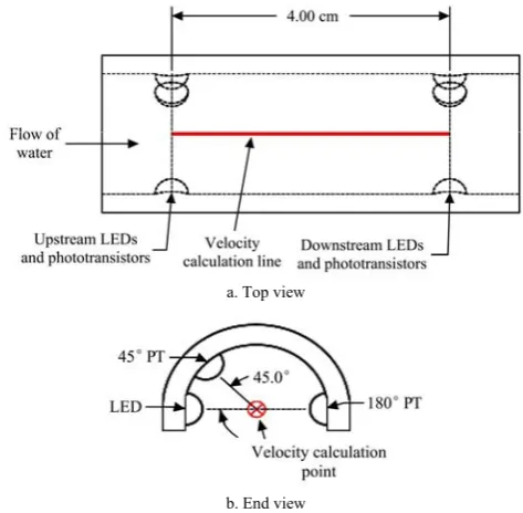
The CFD analysis of the sensor body created a great deal of information about the flows around the sensor. However, only the flow of the water between the upstream and downstream phototransistor/LED pairs affected the velocity measurement because the velocity was determined by the travel time of dye between the pairs. In the simulation, it was assumed that the dye detected by the phototransistors flowed in the center of the sensor directly between the LEDs and 180°
phototransistors along the path highlighted in red and labeled “velocity calculation line” in Figure 4. This assumption was justified for two reasons. First, the shortest flow path would be a straight line between the upstream and downstream locations. This path would be in the center of the channel where boundary layer effects created by the walls of the channel were at a minimum. The dye carried by this flow would be the first to pass the phototransistors to change their signals. Second, the dye flowing along the “velocity calculation line” was the dye that had the greatest effect on the 45° and 180° phototransistors because: (1) this line passed through the center line of the LED where luminous intensity was the highest and (2) it was also the center line of both phototransistors where the sensitivities of the phototransistors were the highest.
a. Top view
b. End view
Figure 4 Close-up view of sensor: LEDs and the line (in Red) used for determining velocity as measured by the sensor 2.3.1 Flow velocity calculation
When built and used in the field, the sensor was programmed to estimate velocity using the travel time and the known distance between the upstream and downstream locations:
sensor measurement travel
d V
t
= (8)
where, Vsensor measurement is the flow velocity as measured
by the sensor, m/s; ttravel is the dye travel time from the
between the upstream and downstream locations (also the length of the velocity calculation line), m.
During sensor operation, the dye travel time was determined using a cross covariance calculation to estimate the time difference between the dye’s effect on the upstream and downstream phototransistors. For the simulation, however, this time was calculated from the simulation results, as explained in the next section. 2.3.2 Flow velocity estimate from the CFD simulation
In the CFD simulation, the velocity along the dye travel path varied from cell to cell within the mesh and the path length within each cell also varied (see Figure 3). Therefore, the travel time within each cell had be calculated first, and the time spent in all cells along the velocity calculation line were added to determine the total travel time, as shown in the denominator of Equation (2). The numerator of Equation (2) is the length of the velocity calculation line represented as the sum of the lengths of that line within each cell.
1 CFD
1 V
N i i
N i
i i
d d V
= =
=
∑
∑
(9)where, VCFD is the average flow velocity within the
velocity calculation line estimated by the CFD simulation, m/s; i is the index for cells in the velocity calculation line;
N is the total number of cells in the mesh along the velocity calculation line; Vi is the velocity of fluid in the
i-th cell along the velocity calculation line, m/s; di is the length of the i-th cell along the velocity calculation line i, m.
VCFD provides a velocity estimate from the CFD
analysis that corresponds to the calculation shown in Equation (1) that was performed by the sensor when installed in the field. Once VCFD was calculated, it was
compared to the free-stream velocity to estimate the potential velocity measurement error caused by the presence of the sensor in the fluid.
The standard analysis techniques embedded within the CFD package do not provide VCFD automatically.
Spatial or volume based averages of various properties are available, but Equation (2) is not a simple spatial average. Equation (9) was integrated into the CFD analysis by adding the following steps: (1) the
velocity-calculation-line shown in Figure 4 was added to the CFD model. (2) The velocity within each cell, Vi, was calculated as the projection of the cell’s velocity vector in the direction of the velocity-calculation-line. (3) The velocity within each cell and the points where the velocity calculation line intersected the cell were then exported from the CFD model for further processing. (4) The points of intersection were then used to calculate the length of the velocity calculation line passing through the cell, di, and, finally, (5) VCFD was calculated using
Equation (2).
2.4 Simulations performed
It was desired that the sensor be able to operate with a free-stream water velocity range of 0.1 m/s to 5.0 m/s with minimal velocity estimation errors. Therefore, the free-stream velocities evaluated were 0.1, 0.25, 0.5, 0.75, 1, 1.5, 2, 2.5, 3, 3.5, 4, 4.5, and 5 m/s. At each of these test velocities, the CFD analysis was used to predict the velocity that would be estimated by the sensor and that velocity was compared to the free-stream velocity.
3 Results
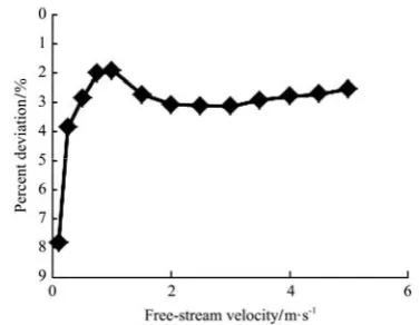
The analysis outlined in the previous section was applied to the original sensor design with the 10 cm extension necessary to ensure the dye flowed through the sensor (Figure 1d). Figure 5 shows the deviation between the velocity measured by this original design according to the CFD model performed with the k-ε
turbulence model and the free-stream velocity. The velocities within the measurement range (0-5 m/s) would all be underestimated by the original sensor design, and the measurement error would reach –8% at low velocities.
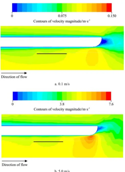
To determine why the velocity measured by the sensor deviated from the free-stream velocity, contour maps (Figure 7) were produced on the vertical cross sectional plane depicted in Figure 6 for all the velocities tested. This cross sectional plane contained the velocity calculation line so the variations along that line could be observed. The velocity contour map on this plane also depicted the flow in regions up- and down-stream of the velocity calculation line, which helped identify what was affecting the flow velocity and causing measurement errors. In general, a certain set of features of the sensor had stronger effects at the lowest free-stream velocities tested (around 0.1 m/s) (Figure 7a), and a different set of features more strongly affected free-stream velocities closer to 5.0 m/s (Figure 7b). In these figures, higher velocities are shown with warmer colors while lower velocities are shown with cooler colors. The vertical cross section intersects only a portion of the sensor body (as illustrated by dark gray region in Figure 6), and therefore, the white region representing the sensor body in the image is thinner than the maximum height of the
a. Front view of the sensor with the contour plane at the center
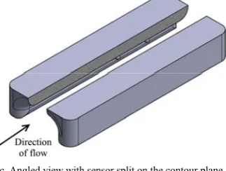
b. Front view of the sensor split on the contour plane
c. Angled view with sensor split on the contour plane
Figure 6 Illustration of location of the cross sectional plane used to produce the velocity contour maps (dark gray represents where
the sensor intersects with the contour plane)
sensor body. These contour maps also illustrate that the volume used for CFD analysis was sufficiently large. The sensor’s effect on the flow remains well away from the upstream and side boundaries of the volume. On the downstream edge of the volume, the sensor’s effect has reached a consistent state and would not produce changes in the flow around the sensor, which was well upstream of this point.
a. 0.1 m/s
b. 5.0 m/s
Figure 7 Velocity contours around original sensor design: at free-stream velocities of 0.1 m/s and 5.0 m/s
increased water velocity (labeled Fast Regions in Figure 7) were caused by the funnel-like geometry of these parts of the sensor. The flow along the velocity calculation line was primarily affected by the boundary layer slow region and the fast region caused by the funnel-like channel exit. The size and the shape of these regions of different local velocities—and thus the deviation from free stream velocity—varied as the free-stream velocity changed. For the original sensor design, in the 0.1 m/s to 5.0 m/s velocity range, the slower boundary layer region always overpowered the faster region at the exit of the sensor, which was why the sensor always underestimated velocity.
a. 0.1 m/s
b. 5.0 m/s
Figure 8 Detailed velocity contours around original sensor design in the region of the velocity calculation line (black line in contour
map): at free-stream velocities of 0.1 m/s and 5.0 m/s Using the CFD analysis to evaluate the effects of design changes, the sensor geometry was improved. The final resulting geometry is shown in Figure 9. To limit the development of a slow region caused by formation of a boundary layer, the sensor was made as short as possible while still maintaining the 10 cm distance between the dye release point and upstream
detection location and the 4 cm distance between detection locations. This meant that the dye release point and the downstream LEDs/phototransistors were located as close as possible to the entrance and exit, respectively. Placing these components so near the ends of the sensor prevented the sensor from having a smooth, streamlined profile. However, the velocity variations produced by the sharp edges were all confined to the top and sides of the sensor, away from the channel. Although limiting the length of the sensor reduced the slow region from the boundary layer, the boundary layer still had an effect. This was mitigated by fast regions produced by a slight curvature at the entrance and exit of the sensor. This curvature is significantly less than that of the original funnel-like design. Repeated CFD analysis was used to evaluate design changes to find the appropriate balance between creation of the fast regions and the boundary layer development at all flow velocities of interest.
Figure 9 Views of improved sensor design (shaded views included for complex geometry)
Figure 10 compares the final design with the original. The final design reduced the measurement error to less than ±4% within the entire velocity range. The analyses used to improve the sensor design were all performed using the k-ε model. The results obtained using this model were checked using the k-ω turbulence model and both results are displayed in Figure 10. The k-ω
turbulence model yielded slightly higher error at the higher velocities than the k-ε turbulence model. The k-ω
k-ε model, the error levels remained within the same ±4% bounds.
Figure 10 Comparison of velocity measured by final sensor to free-stream velocity
The velocity contours around the final design at free-stream velocities of 0.1 m/s and 5.0 m/s are displayed in Figures 11a and 11b, respectively. These contours show that the intensity of the fast regions has been reduced compared to the original design and the size of the slow region that impacts the velocity calculation line has been significantly reduced and no longer reaches the velocity calculation line (Figure 12).
a. 0.1 m/s
b. 5.0 m/s
Figure 11 Velocity contours around final sensor design: at free-stream velocities of 0.1 m/s and 5.0 m/s
a. 0.1 m/s
b. 5.0 m/s
Figure 12 Detailed velocity contours around final sensor design in the region of the velocity calculation line (black line in contour
map): at free-stream velocities of 0.1 m/s and 5.0 m/s
4 Discussion
Identifying a design that minimized errors required testing many different geometries, and the final sensor design was selected only after testing over twenty different geometries. This testing enabled recognition of fluid flow characteristics that affected the velocity estimate and the sensor structures that influenced these characteristics. The most important of these was the development of the boundary layer. Boundary layer development produced lower velocity flow along the surface of the sensor and, in certain circumstances, could reach the velocity calculation line and cause the sensor to underestimate velocities. This underestimation was larger (in terms of percent deviation) at lower free-stream velocities. The influence of the boundary layer was dependent on the length of the sensor with shorter sensor geometries exhibiting a reduced effect from the boundary layer.
funneling structures in the sensor geometry. When these faster flow regions reached the velocity calculation line, they caused an overestimate of flow velocity. The magnitude of the overestimate was dependent on the size of the funneling structures and how close they were to the velocity calculation line. In terms of percent deviation, the effect of these faster flow regions was consistent across the tested velocity range.
A final sensor design characteristic that influenced velocity estimation was the existence of protruding LEDs and phototransistors. While both the original and final design of the sensor had optical components that protruded into the channel, these components could have been mounted flush with channel surface instead. The CFD modeling indicated that protruding LEDs and phototransistors caused underestimation of velocity, but the effect was more pronounced at higher free-stream velocities. Based on these factors, the final design minimized its length to reduce the effect of the boundary layer. It used protruding LEDs and phototransistors to balance the boundary layer’s underestimation at low free-stream velocities with increased underestimation at higher free-stream velocities. Finally, it incorporated a slightly rounded entrance and exit to the channel in the sensor to counteract the underestimation caused by the other factors.
As depicted in Figure 9, the final design was relatively complicated. However, this complexity was not an issue for production using a 3D printer. The Dimension SST1200es (Stratasys, Eden Prairie, Minnesota) was utilized to produce the final design in ABS plastic. This freedom in the production process allowed consideration of a wider variety of complex designs.
The final sensor design was constructed and tested in a natural open channel stream to evaluate overall system function including electronics and data storage. The velocities estimated by the new design (with improved electronics) were compared against an acoustic Doppler velocimeter, the Flowtracker Handheld-ADV from Sontek (San Diego, California). These tests focused on system improvements over the original sensor and were not designed to confirm the error predicted by the CFD
analysis, which, according to the data presented in Figure 10, should be less than 4% at all velocities considered. The field-testing was performed in the intended target environment, a natural stream, so turbulence was present. This turbulence generated noise and variance in the data and limited the ability of the test to determine small percent differences. The CFD models provided solutions based on flows where the turbulence effects are removed through time-averaging so comparisons must to be made to average measurements from the installed sensor which would require a large number of individual measurements at constant stream conditions. The field-testing was focused on capturing a wide variety of flow rates and was not designed to produce the hundreds of velocity measurements that would be necessary to detect a less than 4% average error at all the velocities of interest. Similarly, field tests with the original sensor design were not powerful enough to detect up to 8% error as it could only provide one measurement every few minutes. Although the field-testing could not confirm the CFD results, it did generate useful information on sensor sub-systems and operation which will be presented in other publications.
Further, given that other researchers[10,11] have performed field tests to confirm the ability of CFD to predict errors in sensor operation, yet another confirmation of an established procedure appears unnecessary. Rather, this paper focuses on the applicability of this tool to develop a better sensor design. The long computation times of CFD analysis combined with the large number of variables that could describe possible geometries preclude using an optimization algorithm to create sensor geometries. Therefore, analytical methods such as those described here are necessary to use CFD to improve sensor designs.
5 Conclusions
2%-8% within the velocity range of 0.1 m/s to 5.0 m/s. The final sensor design had a short sensor body that limited boundary layer formation at low free-stream velocities. The entrance and exit to the flow channel on the sensor were sharper than the original design because the rounded entrance and exit created regions of increased velocity. All sharp edges on the surface of the sensor required to support the LEDs and dye injection, were confined to the sides of the sensor, away from the flow channel. This prevented the sharp changes in velocity within the channel where the velocity was measured. The maximum velocity measurement error of the final design as predicted by both the k-ε and k-ω turbulence models was within ±4% for the velocity range of 0.1 m/s to 5.0 m/s.
The original sensor geometry was developed by engineers who focused on creating a relatively smooth profile. Without the benefit of CFD analysis, they were unaware that the large funnel-like entrance and exit generated significant effects on flow characteristics or that these had to be balanced with boundary layer formation to produce accurate readings across the desired velocity range. The CFD simulation was used to predict the velocity measurement expected with potential sensor designs using a mathematical analysis of the results along the velocity calculation line. Velocity contour maps were also used to illustrate potential issues affecting the flow. As a result, a final design that significantly reduced the velocity measurement error was developed. Future researchers developing other sensors for operation in open channels could employ similar methods to ensure their sensor geometries were appropriate and hopefully produce similar improvements.
Acknowledgements
The authors of this paper would like to thank the Environmental Security Technology Certification Program (ESTCP) for funding this research. Also, the NSF GK-12 Program is acknowledged for providing a fellowship for one of the authors during this study.
[References]
[1] Camnasio E, Orsi E. Calibration method of current meters.
J Hydraul Eng, 2011; 137(3): 386–97.
[2] Muste M, Vermeyen T, Hotchkiss R, Oberg K. Acoustic velocimetry for riverine environments. J Hydraul Eng, 2007; 133(12): 1297–8.
[3] Rehmel M. Application of acoustic Doppler velocimeters for streamflow measurements. J Hydraul Eng, 2007; 133(12): 1433–8.
[4] Song Z,Wu T,Xu F,Li R. A simple formula for predicting settling velocity of sediment particles. Water Science and Engineering, 2008; 1(1): 37–43.
[5] Reis S, Seto E, Northcross A, Quinn N W T, Convertino M, Jones R L, et al. Integrating modelling and smart sensors for environmental and human health. Environmental Modelling & Software, 2015; 74: 238–46.
[6] Wong B P, Kerkez B. Real-time environmental sensor data: An application to water quality using web services. Environmental Modelling & Software, 2016; 84: 505–17. [7] Luo H, Li G, Peng W, Song J, Bai Q. Real-time remote
monitoring system for aquaculture water quality. Int J of Agric & Biol Eng, 2015; 8(6): 136–143.
[8] Jin N, Ma R, Lv Y, Lou X. A novel design of water environment monitoring system based on WSN. International Conference on Computer Design and Applications, IEEE, 2010; V2-593-V2-597.
[9] Gartia M R, Braunschweig B, Chang T-W, Moinzadeh P, Minsker B S, Agha G, et al. The microelectronic wireless nitrate sensor network for environmental water monitoring. Journal of Environmental Monitoring, 2012; 14(12): 3068–75.
[10] Mueller D S, Abad J D, Garcia C M, Gartner J W, Garcia M H, Oberg K A. Errors in acoustic Doppler profiler velocity measurements caused by flow disturbance. J Hydraul Eng, 2007; 133(12): 1411–20.
[11] Tokyay T, Constantinescu G, Gonzalez-Casto J A. Investigation of two elemental error sources in boat-mounted acoustic Doppler current profiler measurements by large eddy simulations. J Hydraul Eng, 2009; 135(11): 875–87. [12] Levesque V A, Oberg K A. Computing discharge using the
index velocity method. Techniques and Methods 3–A23. Reston, Va.: U.S. Geological Survey, 2012.
[13] Bigham D. Calibration and testing of a wireless suspended sediment sensor. MS Thesis. Manhattan, Kans.: Kansas State University, 2012.
[14] Zhang N, Dvorak J S, Zhang Y. A correlation-based optical flowmeter for enclosed flows. Transactions of the ASABE, 2013; 56(6): 1511–22.
[15] Dvorak J S, Bryant L E. An optical sprayer nozzle flow rate sensor. Transactions of the ASABE, 2015; 58(2):251–259. [16] Dvorak J S, Stombaugh T S, Wan Y. Nozzle Sensor for
[17] ANSYS. ANSYS FLUENT Users Guide. Release 13.0. Canonsburg, Pa. 2010.
[18] Launder B E, Spalding D B. Lectures in mathematical models of turbulence. New York,: Academic Press; 1972. p 169.
[19] Shih T H, Liou W W, Shabbir A, Yang Z, Zhu J. A new k-ϵ eddy viscosity model for high reynolds number turbulent flows. Computers & Fluids, 1995; 24(3): 227–38.
[20] ANSYS. ANSYS FLUENT Theory Guide. Release 13.0. Canonsburg, Pa.2010.
[21] Wolfshtein M. The velocity and temperature distribution in one-dimensional flow with turbulence augmentation and pressure gradient. Int J Heat Mass Tran, 1969; 12(3): 301–18.
[22] Jongen T. Simulation and modeling of turbulent incompressible fluid flows: École polytechnique fédérale de Lausanne; 1998.
[23] Menter F R. Two-equation eddy-viscosity turbulence models for engineering applications. AIAA Journal, 1994; 32(8): 1598–605.
[24] Fourniotis N T, Toleris N E, Dimas A A, Demetracopoulos A C. Numerical computation of turbulence development in flow over sand dunes. Advances in Water Resources and Hydraulic Engineering. Berlin Heidelberg: Springer; 2009. pp. 843–8.
[25] Blasius H. Grenzschichten in Flüssigkeiten mit kleiner Reibung. Organ für angewantde mathematik, 1908; 56: 1–38.
[26] Blasius H. Das Ähnlichkeitsgesetz bei Reibungsvorgängen in Flüssigkeiten: Springer; 1913.