Convolutional neural network-based automatic image recognition for
agricultural machinery
Kun Yang
1,2,
Hui Liu
1*,
Pei Wang
2,
Zhijun Meng
2,
Jingping Chen
2(1. Information Engineering College, Capital Normal University, Beijing 100048, China;
2. National Engineering Research Center for Information Technology in Agriculture, Beijing 100097, China)
Abstract: An internet of things-based subsoiling operation monitoring system for agricultural machinery is able to identify the type and operating state of a certain machinery by collecting and recognizing its images; however, it does not meet regulatory requirements due to a large image data volume, heavy workload by artificial selective examination, and low efficiency. In this study, a dataset containing machinery images of over 100 machines was established, which including subsoilers, rotary cultivators, reversible plows, subsoiling and soil-preparation machines, seeders, and non-machinery images. The images were annotated in tensorflow, a deep learning platform from Google. Then, a convolutional neural network (CNN) was designed for targeting actual regulatory demands and image characteristics, which was optimized by reducing overfitting and improving training efficiency. Model training results showed that the recognition rate of this machinery recognition network to the demonstration dataset reached 98.5%. In comparison, the recognition rates of LeNet and AlexNet under the same conditions were 81% and 98.8%, respectively. In terms of model recognition efficiency, it took AlexNet 60 h to complete training and 0.3 s to recognize 1 image, whereas the proposed machinery recognition network took only half that time to complete training and 0.1 s to recognize 1 image. To further verify the practicability of this model, 6 types of images, with 200 images in each type, were randomly selected and used for testing; results indicated that the average recognition recall rate of various types of machinery images was 98.8%. In addition, the model was robust to illumination, environmental changes, and small-area occlusion, and thus was competent for intelligent image recognition of subsoiling operation monitoring systems.
Keywords: agricultural machinery, monitoring system, automatic image recognition, convolutional neural network
DOI: 10.25165/j.ijabe.20181104.3454
Citation: Yang K, Liu H, Wang P, Meng Z J, Chen J P. Convolutional neural network-based automatic image recognition for agricultural machinery. Int J Agric & Biol Eng, 2018; 11(4): 200–206.
1 Introduction
Nowadays there have been rapid development and wide application of the Internet of things in intelligent recognition, positioning, monitoring, and management of agricultural machinery cluster operations by using satellite positioning devices, agricultural machinery operation state sensors, and image sensors for real-time detection of machinery operating states based on communication networks and the Internet[1-3]. To promote
farmers to use subsoiling operations that can enhance permeabilities of soil, improve soil physico-chemical properties, grow crop root system environments without disturbing soil layer structure, and facilitate increases in crop yield, the Chinese government has launched subsoiling subsidy programs in a number of provinces. However, there were some problems during implementation of the policy, such as subsoiling quality differences and false declaration of operation areas. As a result, an Internet of
Received date: 2017-04-26 Accepted date: 2018-01-09
Biographies: Kun Yang, MA, research interests: computer vision, Email: [email protected]; Pei Wang, Assistant Research Fellow, research interests: multi-source spatial data analysis in precision agriculture Email: [email protected]; Zhijun Meng, Professor, research interests: intelligent agricultural equipment. Email: [email protected]; Jingping Chen, Senior Engineer, research interests: multi-source spatial data analysis in precision agriculture. Email: [email protected].
*Corresponding author: Hui Liu, Associate Professor, research interests: ICT application in precision agriculture. No.56, North Road of Western 3rd-Ring, P.O.Box 801, Beijing 100048, China. Tel: +86-10-68901370, Email: [email protected].
things-based subsoiling operation supervision system for agricultural machinery was developed to assist the government with machinery subsoiling operation quality supervision based on data from a global positioning system (GPS) and depth sensors, such as machinery path and operation depth[4-6]. Currently, over
13 000 sets of this system have been widely used in 16 provinces and cities, including Anhui, Shandong, and Xinjiang. Automatic recognition of machinery type and operating state by means of image recognition, which is a key technique for subsoiling operation supervision systems, is helpful to reduce the workload of artificial selective examination, strengthen supervision, and improve the intelligence of the system.
Image recognition has been widely applied in agricultural science, such as for the identification of plant diseases and insect pests[7,8], fruit variety identification[9,10], yield estimation[11,12], and
machinery path plans[13]. These have brought changes to
traditional modes of production, and improved work efficiency. Traditional image recognition methods require image features in advance, with feature operators designed based on priori knowledge; then, a classifier is selected for classification based on the actual situation. convolutional neural network (CNN)-based deep learning algorithms[14,15] are designed for classified image
recognition by simulating the connections among neurons to automatically extract image features, which then go through multilayer iteration and feature abstraction based on the feature layering mechanism of the animal visual system. A classical CNN, such as LeNet[16] and AlexNet[17], consists of a convolutional
the convolutional layer; dimension reduction of a feature map is handled in the pooling layer, with major information preserved; then, after several convolution-pooling connections, image features are transformed from detailed edge information to abstract semantic information that then undergoes iteration in the fully connected layer to realize classified recognition[18-20]. CNN
algorithms, without artificial feature extraction, have been favorably applied in various fields including image recognition[21,22], voice recognition[23,24], and natural language
processing[25,26]. A CNN-based image recognition technique
requires a training dataset that covers a large number of annotated images. Current open-source datasets, such as cifar10, cifar100, and IamgeNet, provide data of general objects, such as faces, automobiles, birds, and fish, yet there is not any open-source data set of agricultural machinery.
To achieve automatic recognition of agricultural machinery images, we employed a CNN-based image recognition technique in this study, and we studied the automatic classification method of massive agricultural machinery images. We developed an image annotation dataset of agricultural machinery by collecting and collating relevant images, and then designed a CNN model according to the practical demands of the supervision system and image features of agricultural machinery.
2 Construction of annotated agricultural machinery
image dataset
2.1 Images collection and collation
Agricultural machinery images were collected from subsoiling operation supervision systems. Vehicle-mounted cameras took
images of the machinery every 2 min during operation. Those images were then uploaded to the supervision system via GPRS wireless network. Machinery images of five types of machines (subsoliers, rotary cultivators, subsoiling and soil-preparation machines, reversible plows, and seeders), as well as images of non-machinery, were sorted by analyzing subsoiling operating images taken in various provinces from September to October 2015, thereby constructing a dataset that contained 100 000 agricultural machinery images. Figure 1 shows several types of agricultural machinery. Of all images, 80 000 were used to construct the training dataset and the other 20 000 for data verification. Table 1 shows the distribution of different types of agricultural machinery images in the dataset. The number of each type of machinery image was determined based on the proportion in all original images. The resolution of the original image is 320×240 pixels, in order to accommodate network input, the size of each image in the dataset was converted to 64×64 pixels.
Table 1 Distribution of different types of machinery
Machinery type set/imageTraining Verification set/image Sample size/pixels
Subsoilers 30000 7500 64×64
Subsoiling and
soil-preparation machines 15000 3750 64×64
Seeders 5000 1250 64×64
Reversible plows 8000 2000 64×64
Rotary cultivators 15000 3750 64×64
Abnormal images 7000 1750 64×64
Total 80000 20000 64×64
Figure 1 Agricultural Machinery Images
2.2 Dataset Annotation
Since CNN algorithms belong to supervised classification, annotation of massive data was required. In this study, the machinery image dataset was annotated following tensorflow, a deep learning platform from Google. Firstly, the collated
functions of tensorflow were used to convert each image into a fixed-length binary data, of which the first byte was the image label and other 64×64×3 bytes were image information. Finally, the training set and verification set were converted into 2 independent binary files, thus obtaining the annotated dataset of agricultural machinery.
3 Automatic recognition algorithm of agricultural
machinery image
3.1 Structure of CNN
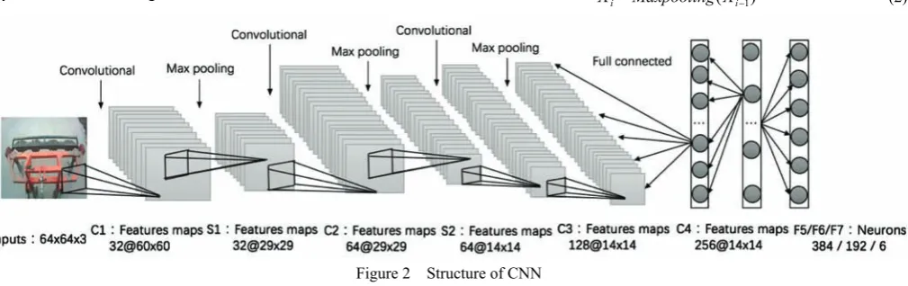
As shown in Figure 2, the CNN structure designed in this study was composed of seven layers, i.e., four convolutional layers and three fully connected layers. The first two convolutional layers were connected to the pooling layers, and the last fully connected layer was classified using the softmax function.
If Xi represented the feature map of the ith layer of the CNN, and network input X0 was the original 64×64×3 image, then the
convolutional layer Xi could be described as
Xi= f(∑iXi−1⊗Wi+bi) (1) where, Wi is the weight vector of the convolutional kernel of the ith layer; the operator ⊗ represented the convolution operation between the convolutional kernel and image of the ith layer or
feature map, with the convolution result added to offset bi; and the feature map of the ith layer is obtained using non-linear excitation
function f(x), a Relu function that features good convergence performance and low computation complexity.
The most common pooling methods include average pooling and max pooling. We employed the latter in this study. If Xi is the pooling layer, Xi could be described as:
1
( )
i i
X =Maxpooling X− (2)
Figure 2 Structure of CNN Table 2 lists the detailed design parameters of the CNN.
There were 32 5×5×3 convolutional kernels in layer C1, with a step length of 1. Thirty-two types of features and 32 60×60 feature maps were extracted after image convolution. Then, 32 29×29 feature maps were obtained after layer S1. Since there were 64 5×5×32 convolutional kernels in layer C2, 64 29×29 could be obtained after convolution of feature maps output by layer S1. Then, 64 14×14 feature maps were obtained after layer S2. Since there were 128 5×5×64 convolutional kernels in layer C3, 128 14×14 could be obtained after convolution of feature maps output by layer S2. Then, since there were 256 5×5×128 convolutional kernels in layer C4, 256 14×14 feature maps could be obtained and exported to layer F5 where 384 neurons were used for fully connected processing of 256 14×14 feature maps. The 192 neurons in layer F6 were used for fully connected processing of 256 neurons. In layer F7, the softmax function was employed to classify eigenvector results into 6 categories.
Table 2 Parameter design of CNN
Layer
Detailed parameters Number of
Features Maps
Size of convolution
kernel
Strides C1 (Convolutional layer 1) 32 5×5 1
S1 (MaxPooling layer 1) 32 3×3 2
C2 (Convolutional layer 2) 64 5×5 1
S2 (MaxPooling layer 2) 64 3×3 2
C3 (Convolutional layer 3) 128 5×5 1 C4 (Convolutional layer 4) 256 5×5 1 F5 (Fully connected layer 1) Number of neurons: 384
F6 (Fully connected layer 2) Number of neurons: 192 F7 (Softmax layer) Number of neurons: 6
3.2 Overfitting reduction
The phenomenon that the CNN model has a high recognition rate of the training set and low recognition rate for the verification set is known as overfitting. This is usually caused by excessive model complexity, inadequate training data, or uneven distribution of training set images. In this study, we used data augmentation and model regularization method to reduce overfitting.
3.2.1 Data augmentation
Two types of dataset enhancement were employed in this study: increasing the volume of the dataset, and improving dataset richness.
The volume of the dataset is the primary condition to reduce overfitting and guarantee network performance. The dataset volume was increased by random cropping and vertical flip: firstly, a 60×60 area was extracted from the center and 4 corners of the image for training, respectively, i.e., the dataset was enlarged by 5 times; Due to different installation method, some machinery images were flipped upside down. To balance the data of these images and improve the model’s recognition capability, all images were vertically flipped, by which the dataset volume was doubled while guaranteeing data richness.
The above two ways improves the richness of dataset, so as to enhance model’s recognition capability of machinery images in various conditions.
3.2.2 Model regularization
Regularization is a method for model complexity reduction. Optimization of the loss function tended to select small parameters as a result of introducing prior distribution when constraint terms are added to the function. The L2 regularization method used in this study also does this; a regularization term was added after the loss function, thereby obtaining a new loss function:
2 0
2 ω
λ
C C ω
n
= +
∑
(3)where, C0 is the original cost function; and 2
2 ω
λ ω
n
∑
is theregularization term, where the square of all parameters ωis divided by the size of the training set sample n, and then multiplied by regularization coefficient λ. This weighs the proportion of the regularization term in the original cost function C0. According to
the parameter update rule of the gradient descent method, the derivative of the new loss function was taken first, by which the updated parameter value ω' could be worked out:
0
0
1
C
ω ω η
ω
C λ
ω η η ω
ω n ηλ C ω η n ω ∂ ′ = − ∂ ∂ ⎛ ⎞ = −⎜ + ⎟ ∂ ⎝ ⎠ ∂ ⎛ ⎞ = −⎜ ⎟ − ∂ ⎝ ⎠ (4)
As seen in Equation (4), there was an attenuation factor
1 ηλ 1
n
⎛ − ⎞< ⎜ ⎟
⎝ ⎠ when the parameter of the loss function was updated.
As a result, L2 regularization is also known as weight reduction, and plays two roles: reducing the impact of important characteristics to avoid poor generalization capability due to the model learning too many characteristics, and guaranteeing that the model has selected smaller parameters with gradient descent so that model complexity can be reduced.
3.3 Improvement of model training efficiency
3.3.1 Image normalization
Image normalization is a method commonly used for dataset pre-processing in computer vision technology, following the basic idea of seeking a group of parameters that are able to eliminate the impact of other transformation functions on image transformation using the image’s invariant moment, i.e., enhancing the image’s affine transformation by transforming it into standard form. In CNN algorithm, UNIT-type data whose pixel value is between 0-255 is normalized to 0-1 to simplify calculation, accelerate network convergence performance, and improve network calculation precision. Normalization can be divided into dispersion normalization and standard deviation:
* x μ
x
σ
−
= (5)
where, μis the average pixel value, and σis the standard deviation of all pixels.
A normalized image is of standard normal distribution when it had a mean value of 0 and standard deviation of 1. Training and prediction of the CNN is conducted according to statistical probability of a sample in the event. The data are normalized to 0-1 for probability distribution statistics. The mean value of all pixels of the sample is 0, and with a consistent standard deviation,
network learning rate and network convergence could be accelerated.
3.3.2 Multi-GPU training
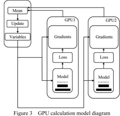
Since there were approximately 20 000 000 parameters mostly generated from fully connected layers and a few generated from convolutional layers to be trained for the machinery recognition model in this study, which involved hundreds of millions of additions and multiplications to process all images, it would take 5-6 d for a traditional CPU to reach convergence of the model via single-thread processing. Such inefficiency is unconducive to parameter modification and network adjustment. However, designed for large-scale and high floating-point data, the GPU computing module had a significantly enhanced operating rate and reduced operating time, owing to its large bandwidth and parallel data computation. Therefore, a 2-GPU parallel computation method was employed in this study to train the network model, as shown in Figure 3.
Figure 3 GPU calculation model diagram
CNN training was aimed to minimize the network’s loss function. The predicted value was obtained after original images underwent forward transmission. The difference between predicted values and actual values was calculated using the square error cost function. En(w,b), i.e., the error function of the nth sample, could be expressed as follows:
2
1
1
( , ) ( )
2
c n n
n k k k
E w b =
∑
= t −y (6)where, n k
t is the kth dimension of the label corresponding to the nth
sample; n k
y is the kth network output corresponding to the nth
sample; c is the number of categories; w is weight; and b is the offset value.
The random gradient descent method was then employed for backward propagation of the loss value, and update network parameters layer-by-layer during training. The parameter update rule is as follows:
( , ) i i
i E w b
W W η
W
∂ = −
∂ (7)
( , ) i i
i E w b b b η
b
∂ = −
∂ (8)
where, Wi is the neuron weight; bi is the offset value of the neuron; η is the learning rate.
0.01. With 8 threads applied, the data was distributed to 2 GPU modules in independent batches. Both GPUs shared the same model parameters and executed synchronously. Since data transmission between 2 GPUs is slow, all parameters obtained were stored and updated in the CPU.
4 Experiment and analysis
4.1 Model training experiment and results
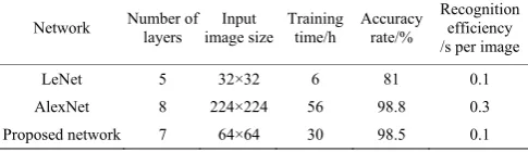
The network model was trained using 2 NVIDIA GeForce GTX 1080 GPU modules in this study. After 100 000 iterations, the loss function was converged to 0.01, and the recognition rate of the model reached 98.2% on the training set and 98.5% on the verification set. For the purpose of comparison, the agricultural machinery image annotation dataset was then trained using LeNet and AlexNet. Table 3 shows parameter configurations and training results of these 3 network.
Table 3 Performance comparison between 3 kinds of CNNs
Network Number of layers
Input image size
Training time/h
Accuracy rate/%
Recognition efficiency /s per image
LeNet 5 32×32 6 81 0.1
AlexNet 8 224×224 56 98.8 0.3
Proposed network 7 64×64 30 98.5 0.1
Table 3 indicates that LeNet featured a simple structure, a small number of network layers, smaller input images, and the lowest training time; however, it had a low recognition rate of 81%, failing to meet practical demands. Both AlexNet and the proposed machinery recognition network were able to meet practical demands with high recognition rates over 98%; however, but AlexNet was a more complicated network that required more parameters and nearly 60 h of training. In comparison, the proposed machinery recognition network boasted a much lower training time, and higher efficiency in testing an image. In summary, the network structure designed in this study could be applied to agricultural machinery recognition, and satisfied actual supervision requirements in terms of network structure and parameters, training time, recognition accuracy, and efficiency.
4.2 Model testing experiment and results
Since there was a great difference in the number of various types of machinery between the training set and verification set, the sample was imbalanced and accuracy inadequate in describing performance in practical application; thus, to construct a verification set for testing, we selected 200 images of each of the 5 types of machinery in various circumstances, such as different brands, illumination conditions, and foreground occlusion, along with an additional 200 non-machinery images taken in Shandong Province in September, 2016. The model was then evaluated with respect to recall rate and robustness.
4.2.1 Confusion matrix and recall rate
Confusion matrices are mainly used to compare a target result and measured value in image recognition accuracy evaluation. If
C[i,j] was a confusion matrix, the jth column represented the
prediction category, and the total number of each column was the number of data that was predicted to be a part of that category; the
ith row was the actual category the data was in, and the total
number of each row stood for the actual number of that category. The value in the matrix was the number of samples actually in category i, but determined to be in category j.
Recall rate is an index evaluating the performance of a classifier. Subset ST was made up of n A-class samples in set S.
When a certain classifier was used for testing S and the samples categorized into class A made up subset S0,
0 T 0
S =S ∩S (9) where, the ratio between m and n (both being the number of elements of S0) was the recall rate of the classifier to A.
Table 4 is elaborated upon as follows:
(1) The value of matrix C[0,0] shows that there were 196 Category 0 recognized as Category 0; the value of matrix C[0,1] means there were 3 Category 0 recognized as Category 1; and the value of matrix C[0,2] indicates that there was 1 Category 0 recognized as Category 2. Therefore, the recall rate of Category 0 (non-machinery images) was 98.0%.
(2) The value of matrix C[1,1] means there were 196 Category 1 recognized as Category 1; the value of matrix C[1,0] means there was 1 Category 1 recognized as Category 0; the value of matrix
C[1,4] suggests that there were 2 Category 1 recognized as Category 4; and the value of matrix C[1,5] indicates there was 1 Category 1 recognized as Category 5. Thus, the recall rate of Category 1(rotary cultivator) was 98.0%.
(3) The value of matrix C[2,2] indicates that there were 197 Category 2 recognized as Category 2; and the value of matrix C[2,4] means there were 3 Category 2 recognized as Category 4. Thus, the recall rate of Category 2 (subsoiling and soil-preparation machine) was 98.5%.
(4) The value of matrix C[3,3] suggests that there were 200 Category 3 recognized as Category 3, which means that the recall rate of Category 3 (reversible plow) reached 100%.
(5) The value of matrix C[4,4] means there were 198 Category 4 recognized as Category 4; and the value of matrix C[4,3] indicates there were 2 Category 4 recognized as Category 3. In other words, the recall rate of Category 4 (subsoiler) was 99.0%.
(6) The value of matrix C[5,5] means there were 199 Category 5 recognized as Category 5; and the value of matrix C[5,4] means there was 1 Category 5 recognized as Category 4. Therefore, the recall rate of Category 5 (seeder) was 99.5%.
Table 4 Confusion Matrix
i 0 1 2 3 4 5 Recall rate/%
0 196 3 1 0 0 0 98.0
1 1 196 0 0 2 1 98.0
2 0 0 197 0 3 0 98.5
3 0 0 0 200 0 0 100
4 0 0 0 2 198 0 99.0
5 0 0 0 0 1 199 99.5 Note: 0-abnormal data, 1-rotary cultivator, 2-subsoiling and soil-preparation machine, 3-reversible plow, 4-subsoiler, 5-seeder.
The average recall rate of all 6 types of images was 98.8%, indicating that this model had favorable robustness and superior practicability due to a high recognition rate to agricultural machinery and correct recognition even with different types of machinery, operating circumstances, non-machinery images, and illumination.
4.2.2 Error analysis
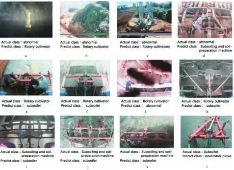
Falsely recognized machinery images were collected, and are shown in Figure 4. The reasons for these false recognitions were determined as follows:
and a subsoiling and soil-preparation machine was falsely recognized as a subsoiler, as shown in Figure 4i.
(2) Soil, crop residues, and people on and around the machinery blocked a large proportion of the machinery, e.g., rotary cultivators were falsely recognized as subsoilers (Figures 4e and 4f), and subsoiling and soil-preparation machines were falsely recognized as subsoilers, as shown in Figures 4h and 4k.
(3) Some machinery had similar shapes, e.g., a subsoiler as shown in Figure4l was falsely recognized as a reversible plow because both machines shared a similar triangular framework and the only difference was that the subsoiler was equipped with a subsoiling shovel.
(4) Inadequate data collection (Figures 4a-4d), and non-machinery images were falsely recognized as rotary cultivators because although they rare, such abnormal images were similar to rotary cultivator in terms of texture and color proportions.
The above analysis suggested some deficiencies in the model: (1) It was weak in recognizing parts some certain machinery or failed to correctly recognize the machinery when there was large-area occlusion or only part of the machinery appeared in the image.
(2) The abnormal image dataset was still inadequate, which resulted in incorrect recognition of some abnormalities.
Figure 4 Falsely-recognized agricultural machinery images
5 Conclusions
1) We constructed an agricultural machinery image annotation dataset covering 6 types of images of over 100 kinds of machinery, i.e., subsoilers, rotary cultivators, reversible plows, subsoiling and soil-preparation machines, and seeders, along with abnormal data. There were 80 000 images in the training set and 20,000 in the verification set. This dataset could be intelligently used for automatic recognition, detection, and tracking of agricultural machinery.
2) A CNN able to automatically recognize agricultural machinery was designed based on practical requirements and data characteristics. The machinery recognition network model whose recognition accuracy reached over 98% and recognition efficiency was 0.1 s/image was obtained with nearly 30 h of training on 2 GPU modules using 80 000 images. The fact that recognition rates of both the training set and verification set reached over 98%
indicated that the network was robust to environmental changes, illumination, and small-area foreground occlusion. It also showed excellent generalization performance since the samples of the training set and verification set did not overlap.
3) Compared with classic LeNet and AlexNet networks, the machinery recognition network developed in this study featured a simpler structure, fewer parameters, and a shorter training time, all while maintaining high recognition accuracy and efficiency.
4) Apart from the training set and verification set, 200 images were randomly selected from each of the 6 types to construct a test set in order to verify the practicability of the model. Test results indicated that the recall rate of various types of machinery images reached an average of 98.8%, indicating superior practicability of the model.
terminals. This was followed by designing a CNN structure and model training, upon which automatic machinery recognition that satisfied practical demands was realized. Follow-up studies will focus on local recognition to further improve the model’s capability to recognize machinery types.
Acknowledgements
This study was financially supported by National Nature Science Foundation of China (Grant No. 31571563 and 31571564), The National Key Research and Development Program of China (Grant No.2016YFD0700303)
[References]
[1] He Y, Nie P C, Liu F. Advancement and trend of internet of things in agriculture and sensing instrument. Transactions of the CSAM, 2013; 44(10): 216–226. (in Chinese)
[2] Qin H B, Li D L, Guo L. Recent advances in development and key technologies of internet of things in agriculture. Journal of Agricultural Mechanization Research, 2014; 4: 246–248. (in Chinese)
[3] Li J, Guo M R, Gao L L. Application and innovation strategy of agricultural internet of things. Transactions of the CSAE, 2015; 31(S2): 200–209. (in Chinese)
[4] Liu Y H, Yuan Y W, Zhang J N, Wang F Z, Niu K. Design and experiment of remote management system for subsoiler. Transactions of the CSAM, 2016; 47(S1): 43–48. (in Chinese)
[5] Zhang X D. Design and implementation of subsoiling monitoring and service system of agricultural machinery based on the android. Shandong Agricultural University, 2016. (in Chinese)
[6] Yin Y X, Meng Z J, Mei H B, Luo C H. Study on tilling depth detection method based on attitude measurement for subsoiler. National Engineering Research Center for Information Technology in Agriculture, Beijing, China, 2015; pp.1331–1337. (in Chinese)
[7] Deng J Z, Li M, Yuan Z B, Jing J, Huang H S. Feature extraction and classification of Tilletia diseases based on image recognition. Transactions of the CSAE, 2012; 28(3): 172–176. (in Chinese)
[8] Wen Z Y, Cao L P. Image recognition of navel orange diseases and insect pests based on compensatory fuzzy neural networks. Transactions of the CSAE, 2012; 28(11): 152–157. (in Chinese)
[9] Tan K Z, Chai Y H, Song W S, Cao X D. Identification of soybean seed varieties based on hyperspectral image. Transactions of the CSAE, 2014; 30(9): 235–242.
[10] Tao H W, Zhao L, Xi J, Yu L, Wang T. Fruits and vegetables recognition based on color and texture features. Transactions of the CSAE, 2014; 30(16): 305–311. (in Chinese)
[11] Qian J P, Li M, Yang X T, Wu B G, Zhang Y, Wang Y N. Yield estimation model of single tree of Fuji apples based on bilateral image
identification. Transactions of the CSAE, 2013; 29(11): 132–138. (in Chinese)
[12] Jia H L, Wang G, Guo M Z, Shah D, Jiang X M, Zhao J L. Methods and experiments of obtaining corn population based on machine vision. Transactions of the CSAE, 2015; 31(3): 215–220.
[13] Zhang T M, Zhuang X L. Identification and navigation system of farmland path for high-clearance vehicle based on DM642. Transactions of the CSAE, 2015; 31(4): 160–167. (in Chinese)
[14] Lecun Y, Bengio Y, Hinton G. Deep learning. Nature, 2015; 521(7553): 436–444.
[15] Schmidhuber J. Deep learning in neural networks: An overview. Neural Networks, 2014; 61: 85–117.
[16] Haykin S, Kosko B. Gradient based learning applied to document recognition. Wiley-IEEE Press, 2009; 86(11): 306–351.
[17] Krizhevsky A, Sutskever I, Hinton G E. ImageNet classification with deep convolutional neural networks. International Conference on Neural Information Processing Systems. Curran Associates Inc. 2012; pp.1097–1105.
[18] Dan C C, Meier U, Gambardella L M, Schmidhuber J. Convolutional Neural Network Committees for Handwritten Character Classification. International Conference on Document Analysis and Recognition. IEEE, 2011; pp.1135–1139.
[19] Szegedy C, Liu W, Jia Y, Sermanet P, Reed S, Angueloy D, et al. Going deeper with convolutions. IEEE Conference on Computer Vision and Pattern Recognition. IEEE Computer Society, 2015; pp.1–9.
[20] Bluche T, Ney H, Kermorvant C. Feature extraction with convolutional neural networks for handwritten word recognition. International Conference on Document Analysis and Recognition. IEEE, 2013; pp.285–289.
[21] He H, Shao Z, Tan J. Recognition of car makes and models from a single traffic-camera image. IEEE Transactions on Intelligent Transportation Systems, 2015; 16(6): 3182–3192.
[22] Liu Z, Luo P, Qiu S, Wang X, Tang X. DeepFashion: Powering robust clothes recognition and retrieval with rich annotations. IEEE Conference on Computer Vision and Pattern Recognition. IEEE Computer Society, 2016; pp.1096–1104.
[23] Noda K, Yamaguchi Y, Nakadai K, Okuno H G, Ogata T. Audio-visual speech recognition using deep learning. Applied Intelligence, 2015; 42(4): 722–737.
[24] Bahdanau D, Chorowski J, Serdyuk D, Brakel P, Bengio Y. End-to-end attention-based large vocabulary speech recognition. IEEE International Conference on Acoustics, Speech and Signal Processing. IEEE, 2016; pp.4945–4949.
[25] Hu B, Lu Z, Li H, Cai Q, Chen Q. Convolutional neural network architectures for matching natural language sentences. Advances in Neural Information Processing Systems, 2015; 3: 2042–2050.