Advanced Techniques for Automatic Change Detection in Multitemporal Hyperspectral Images

Full text

(1)PhD Dissertation. International Doctorate School in Information and Communication Technologies. DISI - University of Trento. ADVANCED TECHNIQUES FOR AUTOMATIC CHANGE DETECTION IN MULTITEMPORAL HYPERSPECTRAL IMAGES. Sicong Liu. Advisor: Prof. Lorenzo Bruzzone Università degli Studi di Trento Co-Advisor: Prof. Peijun Du. Dr. Francesca Bovolo. Nanjing University. Fondazione Bruno Kessler. February 2015.

(2) ii.

(3) If I have seen further, it is by standing on the shoulders of giants. -Isaac Newton.

(4) Dedicated to my mother.. iv.

(5) Abstract. The increasing availability of the new generation remote sensing satellite hyperspectral images provides an important data source for Earth Observation (EO). Hyperspectral images are characterized by a very detailed spectral sampling (i.e., very high spectral resolution) over a wide spectral wavelength range. This important property makes it possible the monitoring of the land-cover dynamic and environmental evolution at a fine spectral scale. This also allows one to potentially detect subtle spectral variations associated with the land-cover transitions that are usually not detectable in the traditional multispectral images due to their poor spectral signature representation (i.e., generally sufficient for representing only the major changes). To fully utilize the available multitemporal hyperspectral images and their rich information content, it is necessary to develop advanced techniques for robust change detection (CD) in multitemporal hyperspectral images, thus to automatically discover and identify the interesting and valuable change information. This is the main goal of this thesis. In the literature, most of the CD approaches were designed for multispectral images. The effectiveness of these approaches, to the complex CD problems is reduced, when dealing with the hyperspectral images. Accordingly, the research activities carried out during this PhD study and presented in this thesis are devoted to the development of effective methods for multiple change detection in multitemporal hyperspectral images. These methods consider the intrinsic properties of the hyperspectral data and overcome the drawbacks of the existing CD techniques. In particular, the following specific novel contributions are introduced in this thesis: 1) A theoretical and empirical analysis of the multiple-change detection problem in multitemporal hyperspectral images. Definition and discussion of concepts as the changes and of the change endmembers, the hierarchical change structure and the multitemporal spectral mixture is given. 2) A novel semi-automatic sequential technique for iteratively discovering, visualizing, and detecting multiple changes. Reliable change variables are adaptively generated for the representation of each specific considered change. Thus multiple changes are discovered and discriminated according to an iterative re-projection of the spectral change vectors into new compressed change representation domains. Moreover, a simple yet effective tool is developed allowing user to have an interaction within the CD procedure. 3) A novel partially-unsupervised hierarchical clustering technique for the separation and identification of multiple changes. By considering spectral variations at different processing levels, multiple change information is adaptively modelled and clustered according to spectral homogeneity. A manual initialization is used to drive the whole hierarchical clustering procedure; 4) A novel automatic multitemporal spectral unmixing approach to detect multiple changes in hyperspectral images. A multitemporal spectral mixture model is proposed to analyse the spectral variations at sub-pixel level, thus investigating in details the spectral composition of change and no-. i.

(6) change endmembers within a pixel. A patch-scheme is used in the endmembers extraction and unmixing, which better considers endmember variability. Comprehensive qualitative and quantitative experimental results obtained on both simulated and real multitemporal hyperspectral images confirm the effectiveness of the proposed techniques. Keywords Change detection (CD), change visualization, change representation, change vector analysis, spectral unmixing, hyperspectral (HS) images, multiple changes, multitemporal analysis, remote sensing, hierarchical analysis.. ii.

(7) iii.

(8) Contents. ABSTRACT…………………………………………………………………………….….......…….…….i LIST OF FIGURES……………………………………………………………………………….…….viii LIST OF TABLES………………………………………………………………………………….….....xi LIST OF ABBREVIATIONS……………………………………………………………….………..…xii LIST OF NOTATION…………………………………………………………………..…….…...……xiv CHAPTER 1 INTRODUCTION............................................................................................................... 1 1.1 INTRODUCTION TO HYPERSPECTRAL REMOTE SENSING SYSTEMS .................................................... 1 1.2 MOTIVATION OF THE THESIS .............................................................................................................. 6 1.3 OBJECTIVES OF THE THESIS ................................................................................................................ 8 1.4 NOVEL CONTRIBUTIONS OF THE THESIS ............................................................................................ 9 1.5 STRUCTURE OF THE THESIS .............................................................................................................. 11 CHAPTER 2 STATE-OF-THE-ART: CHANGE DETECTION TECHNIQUES ............................. 13 2.1 CHANGE DETECTION TECHNIQUES FOR MULTITEMPORAL MULTISPECTRAL IMAGES .................... 13 2.2 CHANGE DETECTION TECHNIQUES FOR MULTITEMPORAL HYPERSPECTRAL IMAGES .................... 17 2.3 PROBLEMS AND CHALLENGES .......................................................................................................... 18 CHAPTER 3 PROPOSED CONCEPTS FOR CHANGE DETECTION IN HYPERSPECTRAL IMAGES .................................................................................................................................................... 21 3.1 ANALYSIS OF THE SPECTRAL DIFFERENCE DOMAIN ........................................................................ 21 3.2 ANALYSIS OF THE SPECTRAL STACKED DOMAIN............................................................................. 24 CHAPTER 4 A NOVEL SEQUENTIAL SPECTRAL CHANGE VECTOR ANALYSIS FOR DISCOVERING AND DETECTING MULTIPLE CHANGES IN HYPERSPECTRAL IMAGES 29 4.1 INTRODUCTION ................................................................................................................................. 29 4.2 MULTIPLE-CHANGE DETECTION BY C2VA IN MULTI/HYPER-SPECTRAL IMAGES ........................... 31 4.2.1 Standard C2VA ......................................................................................................................... 31 4.2.2 Problems and Challenges When Applying C2VA to CD-HS Cases ......................................... 33 4.3 PROPOSED APPROACH ...................................................................................................................... 33 4.3.1 Proposed 2-D Adaptive Spectral Change Vector Representation (ASCVR) ............................ 34 4.3.2 Proposed Sequential Spectral Change Vector Analysis (S2CVA) ............................................ 36 4.4 DATA SET DESCRIPTION AND DESIGN OF EXPERIMENTS ................................................................. 39 iv.

(9) 4.4.1 Description of Data Sets ............................................................................................................39 4.4.2 Design of Experiments ..............................................................................................................42 4.5 EXPERIMENTAL RESULTS ..................................................................................................................42 4.5.1 Simulated Hyperspectral Remote Sensing Data Set ..................................................................42 4.5.2 Simulated Hyperspectral Camera Data Set................................................................................46 4.5.3 Real Hyperion Remote Sensing Satellite Data Set ....................................................................49 4.6 DISCUSSION AND CONCLUSIONS .......................................................................................................53 CHAPTER 5 A NOVEL UNSUPERVISED HIERARCHICAL CLUSTERING METHOD FOR CHANGE DETECTION IN HYPERSPECTRAL IMAGES ................................................................55 5.1 INTRODUCTION ..................................................................................................................................55 5.2 PROPOSED APPROACH .......................................................................................................................56 5.2.1 Pseudo-Binary Change Detection ..............................................................................................57 5.2.2 Hierarchical Spectral Change Vector Analysis (HSCVA) ........................................................58 5.2.3 Generation of the Change-Detection Map by Endmember Clusters Merging ...........................63 5.3 DATA SET DESCRIPTION AND DESIGN OF EXPERIMENTS ..................................................................64 5.3.1 Description of Data Sets ............................................................................................................64 5.3.2 Design of Experiments ..............................................................................................................66 5.4 EXPERIMENTAL RESULTS ..................................................................................................................67 5.4.1 Simulated Hyperspectral Data Set .............................................................................................67 5.4.2 Hyperion Satellite Images of an Irrigated Agricultural Area.....................................................70 5.4.3 Hyperion Images of a Wetland Agricultural Area .....................................................................71 5.5 DISCUSSION AND CONCLUSIONS .......................................................................................................71 CHAPTER 6 A NOVEL UNSUPERVISED MULTITEMPORAL SPECTRAL UNMIXING FOR DETECTING MULTIPLE CHANGES IN HYPERSPECTRAL IMAGES .......................................75 6.1 INTRODUCTION ..................................................................................................................................75 6.2 PROPOSED APPROACH .......................................................................................................................77 6.2.1 Stacking of Multitemporal Images and Image-Patch Generation ..............................................77 6.2.2. Multitemporal Spectral Unmixing (MSU)................................................................................78 6.2.3. Change Analysis .......................................................................................................................79 6.2.4. Abundance Combination and Final Change-Detection Map Generation .................................81 6.3 DATA SET DESCRIPTION AND DESIGN OF EXPERIMENTS ..................................................................81 6.4 EXPERIMENTAL RESULTS ..................................................................................................................83 6.4.1 Simulated Hyperspectral Data Set .............................................................................................83 6.4.2 Real Hyperion Remote Sensing Satellite Data Set ....................................................................88 6.5 DISCUSSION AND CONCLUSIONS .......................................................................................................92. v.

(10) CHAPTER 7 CONCLUSIONS ............................................................................................................... 93 LIST OF PUBLICATIONS ..................................................................................................................... 96 BIBLIOGRAPHY..................................................................................................................................... 98 APPENDIX A.......................................................................................................................................... 105 APPENDIX B .......................................................................................................................................... 106. vi.

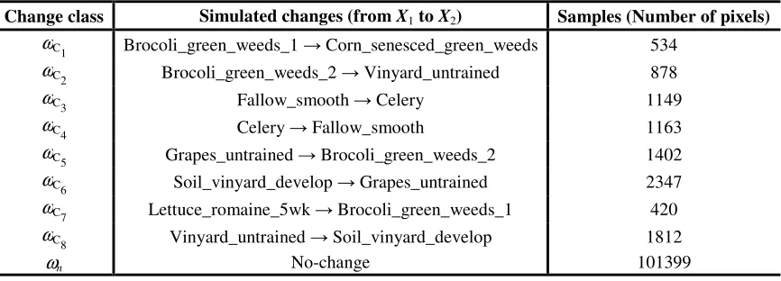
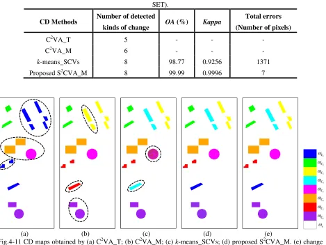
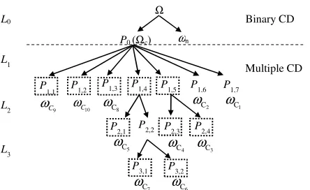
(11) List of Figures. 1-1. A comparison of the measured spectral signature ranges between the hyperspectral EO-1 Hyperion sensor and the multispectral Landsat ETM sensor. .....................................................3. 1-2. Hyperspectral data cube and examples of pixel spectral signatures associated to three landcover materials. ...........................................................................................................................4. 1-3. Heaps’ law of vocabulary growth ...............................................................................................5. 1-4. The whole change-detection processing chain. ...........................................................................6. 1-5. Examples of two change-detection applications. ........................................................................7. 3-1. Example of the SCV signatures associated to three change classes in XD. ...............................22. 3-2. Qualitative illustration of the statistical distribution of the magnitude of SCVs and the sample spectra on SCVs of major changes and subtle changes in XD. ..................................................23. 3-3. Possible change situations of a single pixel in the bi-temporal images based on the pure spectrum and mixed spectrum assumptions. .............................................................................25. 3-4. Illustration of the CD-HS problem in the B-Dimensional difference domain XD and the 2BDimensional multitemporal (stacked) domain XS. ....................................................................26. 3-5. Examples of spectral signatures in the multitemporal domain XS: (a) change and (b) no-change classes........................................................................................................................................27. 4-1. Compressed Change Vector Analysis (C2VA) for representing multiple-changes in the 2-D polar domain. ............................................................................................................................32. 4-2. Block scheme of the proposed CD approach based on S2CVA. ...............................................34. 4-3. Block scheme of the proposed S2CVA step. .............................................................................36. 4-4. Example of the obtained three-level hierarchical tree by the proposed S2CVA........................38. 4-5. The AVIRIS Salinas data set and the reference ground truth data ............................................38. 4-6. False color composite of the real HS image acquired by the AVIRIS sensor in Salinas scenario and the simulated changed image and the change reference map. ............................................40. 4-7. False color composite of the HS image acquired by the Nuance FX HS camera and the simulated image with changes and the Change reference map. ................................................40. 4-8. Real bi-temporal Hyperion images acquired on an agricultural scenario. ................................41. 4-9. Change representation obtained by C2VA_M and by proposed S2CVA_M (simulated hyperspectral remote sensing data set.). ....................................................................................43. 4-10 Three-level hierarchical tree obtained by the proposed S2CVA_M method (simulated hyperspectral remote sensing data set). ....................................................................................44 4-11 CD maps obtained by different apporaches (simulated HS remote sensing data set). ..............45 4-12 Summary of the computational time taken by the proposed technique (in second) on the Salinas simulated hyperspectral data set...................................................................................46 4-13 Change representation obtained by the C2VA_M and the proposed S2CVA_M (simulated hyperspectral camera data set) ..................................................................................................47. vii.

(12) 4-14 Four-level hierarchical tree obtained by the proposed S2CVA_M method (simulated hyperspectral camera data set) ................................................................................................. 48 4-15 Summary of the computational time taken by the proposed technique (in second) on the simulated hyperspectral camera data set. ................................................................................. 49 4-16 Change representations obtained by the C2VA_M and the proposed S2CVA_M approach (real HS Hyperion remote sensing data set). .................................................................................... 50 4-17 Four-level hierarchical tree obtained by proposed S2CVA_M method (real Hyperion remote sensing data set). ...................................................................................................................... 51 4-18 Summary of the computational time taken by the proposed technique (in second) on the real Hyperion hyperspectral data set. .............................................................................................. 53 4-19 Change-detection maps obtained by different approaches (real HS Hyperion remote sensing data set). ................................................................................................................................... 53. 5-1. Block scheme of the proposed change-detection approach to multitemporal hyperspectral images. ..................................................................................................................................... 56. 5-2. Block scheme of the pseudo-binary CD step used for initializing the tree structure................ 58. 5-3. Example of the proposed hierarchical tree for the detection of change endmembers with tree depth D=4 and 8 identified leaves. ........................................................................................... 59. 5-4. Example of definition of the initial cluster number (k0) based on analyzing of the compressed change direction. ...................................................................................................................... 62. 5-5. Block scheme of the HSCVA step in the proposed change-detection approach. ..................... 63. 5-6. False color composite of the HS image acquired by the Nuance FX HS camera (X1) and one of the simulated image (X2) with changes and the reference map ................................................ 64. 5-7. Hyperion images acquired on an irrigated agricultural area. .................................................... 65. 5-8. Hyperion images acquired on a wetland area in China. ........................................................... 65. 5-9. CD results obtained by different approaches on the simulated HS data set. ............................ 68. 5-10 CD results obtained by different approaches on the real Hyperion HS images on an agricultural area. ...................................................................................................................... 70 5-11 CD results obtained by different approaches on the real Hyperion images on a coastal wetland agricultural area in China. ........................................................................................................ 72 6-1. Architecture of the proposed CD approach based on multitemporal spectral unmixing. ......... 77. 6-2. False color composites of the HS image acquired by the AVIRIS sensor in Salinas scenario (X1) and the simulated changed image (X2) and the change reference map ............................. 82. 6-3. Bi-temporal Hyperion images acquired on an agricultural irrigated scenario. ......................... 83. 6-4. Extracted MT-EMs by the proposed MSU approach (simulated data set with SNR=20dB) ... 84. 6-5. Spectral signatures of the MT-EMs extracted by the proposed MSU approach on the simulated data set (SNR=20 dB). ............................................................................................................. 85. 6-6. Final class abundances on the simulated data set (SNR=20dB) ............................................... 85. 6-7. Change-detection maps obtained by the MSU approach on different simulated HS data sets (with SNR=10, 20, 30, 40 dB) ................................................................................................. 86. 6-8. MT-EMs extracted by the proposed MSU approach on the real bitemporal Hyperion data set88 viii.

(13) 6-9. Spectral signatures of MT-EMs extracted by the proposed MSU approach on the real bitemporal Hyperion remote sensing data set ..............................................................................89. 6-10 Final class abundances obtained by MSU on the real bi-temporal Hyperion data set ..............90 6-11 Circle roads that surround the agricultural irrigated fields observed from Google Maps .........90 6-12 Change-detection maps obtained by the considered approaches on the real bitemporal Hyperion data set. .....................................................................................................................91. ix.

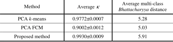
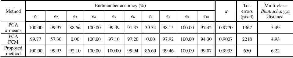
(14) List of Tables. 1-1. Parameters of eight considered hyperspectral instruments ......................................................... 2. 4-1. Simulated changes in salinas data set and the corresponding number of samples ................... 39. 4-2. Number of detected kinds of change, accuracy and error indices obtained by the considered methods (simulated hyperspectral remote sensing data set). ................................................... 45. 4-3. Number of detected kinds of change, detection accuracy and error indices obtained by the considered methods (simulated hyperspectral camera data set). ............................................. 48. 4-4. Number of detected kinds of change in the considered methods (real hyperion remote sensing data set). ................................................................................................................................... 52. 5-1. x-means algorithm for the automatical change clustering. ....................................................... 61. 5-2. Average kappa accuracy and multi-class bhattacharyya distance obtained by the three considered methods on the simulated data sets........................................................................ 67. 5-3. Kappa accuracy, number of detection errors and multi-class bhattacharyya distance obtained by three considered methods on one of the simulated data sets............................................... 69. 6-1. Simulated change classes and related number of samples (salinas data set) ............................ 82. 6-2. Change detection accuracy and error indices obtained by the considered methods (different simulated hs data sets). ............................................................................................................ 87. A-1 Properties of euclidean distance and spectral angle distance ................................................. 105. x.

(15) List of Abbreviations EO RS SAR LiDAR HS MS CD CD-MS CD-HS S2CVA MSU PCC DMC SVM PCA FCM GKC GA SA MRF GS KT MAD CCA IR-MAD CVA C2VA MAPs SFA CE QCE WDS MAD MAF MNF T-PCA ICA UFD stICA SAM SID SCM HOOI SNR SCV MKT MGS MT-EMs LMM SAD ASCVR. Earth Observation Remote Sensing Synthetic Aperture Radar Light Detection And Ranging Hyperspectral Multispectral Change Detection Change Detection in Multispectral images Change Detection in Hyperspectral images Sequential Spectral Change Vector Analysis Multitemporal Spectral Unmixing Post-Classification Comparison Direct Multi-date Classification Support Vector Machine Principal Component Analysis Fuzzy C-Means Gustafson-Kessel Clustering Genetic Algorithm Simulated Annealing Markov Random Fields Gramm-Schmidt Tasselled-cap Transformation Multivariate Alteration Detection Canonical Correlation Analysis Iterative Reweighted MAD Change Vector Analysis Compressed Change Vector Analysis Morphological Attribute Profiles Slow Feature Analysis Covariance-Equalization Class-conditional CE Wavelength Dependent Segmentation Multivariate Alteration Detection Maximum Autocorrelation Factor Minimum Noise Fraction Temporal-Principal Component Analysis Independent Component Analysis Uniform Feature Design Spatio-temporal ICA Spectral Angle Measure Spectral Information Divergence Spectral Correlation Measure Higher Order Orthogonal Iteration Signal-to-Noise Ratio Spectral Change Vector Multi-date Kauth-Thomas Multi-date Graham-Schimidt Multitemporal Endmembers Linear Mixture Model Spectral Angle Distance Adaptive Spectral Change Vector Representation. xi.

(16) SVD USGS C2VA_T C2VA_M k-means_SCVs S2CVA_M OA Kappa EM HSCVA PCs BIC AIC MDL MU HFC NWHFC HySIME ELM VCA ANC. Singular Value Decomposition U.S. Geological Survey Automatic Thresholding in the C2VA feature space Manual (interactive) change identification in the C2VA feature space k-means clustering on the whole changed SCVs S2CVA approach using Manual (interactive) change identification at each level of the representation Overall Accuracy Kappa Coefficient Expectation Maximization Hierarchical Spectral Change Vector Analysis Principal Components Bayesian Information Criterion Akaike Information Criterion Minimum Description Length Multitemporal Unmixing Harsanyi-Farrand-Chang Noise Whitened Version of HFC Hyperspectral Signal Identification by Minimum Error Eigenvalue Likelihood Maximization Vertex Component Analysis Abundance Nonnegative Constraint. xii.

(17) List of Notations I J B p Hf(·) VR LD W, η X1, X2 XD x1(i, j) x2(i, j) Ω Ωc. ωn ωck K Ωe ek XS ES AS NS E1, E2 A1, A2 N1, N2. ρ α D. ρmax Tρ SCn SAc Tα,k R Lh Jh H Ph,j Rh,j Xh,j. Γh,j E[xh,j] Wh,j Vh,j. λhb, j Dh,j ρh,j. Length of the image Width of the image Number of the spectral channels (bands) of the considered images Number of targets (classes) Hidden function Distinct terms in documents Length of documents Free parameters in the formulation of Heaps’ law Hyperspectral images acquired at time 1 and 2, respectively Spectral difference image Pixel with spatial position (i, j) in X1 Pixel with spatial position (i, j) in X2 All classes present in the considered images Set of multiple change classes No-change class k-th change classes in Ωc Number of change classes in Ωc Set of change endmembers k-th change endmember associated to change class ωck Multitemporal stacked image Matrix of the multitemporal-endmember (MT-EM) set in XS Abundance matrix of ES in the linear mixture model Noise matrix in the linear mixture model Matrix of endmember set in X1 and X2, respectively Abundance matrix of E1, E2 in a linear mixture model, respectively Noise matrix in the linear mixture model of X1 and X2, respectively Change magnitude Change direction 2-Dimensional polar coordinate domain Maximum value of ρ Threshold value on the change magnitude ρ Region associated to the unchanged SCVs in the C2VA representation Region associated to the changed SCVs in the C2VA representation k-th threshold value on the change direction α Reference vector h-th level of S2CVA hierarchy Maximum number of change clusters at level Lh Total number of levels in the S2CVA hierarchy j-th change cluster observed in ASCVR at the level Lh Reference vector of ASCVR for cluster Ph,j SCVs associated to cluster Ph,j Covariance matrix of xh,j Expectation of xh,j Diagonal matrix with eigenvalues Matrix of eigenvectors b-th eigenvalue sorted in descending order in Dh,j 2-Dimensioanl representation domain for Ph,j Constructed change magnitude variable for Ph,j. xiii.

(18) αh,j en Ωu δ h(ρ) ρ(i,j) Ld D SΩc. Constructed change direction variable for Ph,j No-change endmember Set of uncertain pixels A margin value on the threshold Tρ Histogram of magnitude ρ Change magnitude value for pixel x(i,j) d-th level of the HSCVA tree structure Depth of the HSCVA tree Reference spectrum calculated by averaging all SCVs in Ωc. ϑ ( x(i, j ), SΩ ). Spectral angle distance between x(i,j) and SΩc. σϑ. Standard deviation value of ϑ ( x(i, j ), SΩc ). Tσ Q(i,j) M H k0 t. Threshold value on σ ϑΩc Selected principal components with spatial position (i,j) Number of the selected PCs Range of number k Initial number of k (i.e., lower bound of H) A constant value to control the upper bound of H. Qk. Pixel data of PCs belong to class. f(·). probability density function M-dimensional normal distribution M-dimensional mean vector M×M dimensional covariance matrix Number of pixel in Qk Likelihood function Maximum likelihood estimate of Θk, µk and Γk. c. Ωc. Θk µk Γk nk Lf Θˆ k , µˆ k , Γˆ k L′f k’ kt ϕ(Q(i,j)) S eε. Bα,β. µα Γα κ P1 P2 Ps XS,z Z Ps,z ES,z U ep ap Uc Un Ωn Ps,c Ps,n r. ωc. k. Likelihood function of the joint probability density function Optimal number of major changes Temporary number of major changes Compressed change direction for Q(i,j) Reference spectrum of endmember eε∈{Ωe, en} Bhattacharyya distance between eα and eβ Mean vector of eα Covariance matrix of eα Kappa coefficient Number of endmembers in X1 Number of endmembers in X2 Number of MT-EMs in XS z-th patch of XS Defined number of patches Number of MT-EMs in patch XS,z Identified set of MT-EMs in patch XS,z Endmember pool Spectral signature of the p-th (p=1,…, Ps) endmember in XS Fractional abundance of ep Endmember pool of change classes Endmember pool of no-change classes Set of no-change classes Number of endmembers in Uc Number of endmembers in Un Probability vector of a given MT-EM eα xiv.

(19) m. θ K'. Probability vector of a given MT-EM eβ SID-SAM combined spectral measure Total number of classes of MT-EMs in XS. ωε. A given class in Ω = ωc1 , ωc2 ,K,ωcK ,ωn. AS,ε AS,p aωε (i, j ). Final abundance map of the class ωε Abundance map of a given MT-EM ep, ep∈ωε Abundance value of class ωε in pixel xs(i,j) Euclidean distance Spectral angle distance Two constant values. {. ∆. ϑ a, b U hs, j Vhs, j ,. (V ) s h, j. Dhs, j. ∗. }. Unitary matrices represent sets of ‘left’ and ‘right’ orthonormal bases in SVD Conjugate transpose of the unitary matrix Vhs, j Diagonal matrix in SVD. xv.

(20) xvi.

(21) Chapter 1. Introduction In this chapter the basic concepts of remote sensing systems, change detection techniques, and hyperspectral sensors are briefly overviewed. The considered challenging multiple change detection problem in multitemporal hyperspectral images is introduced by comparing with the same problem on the traditional multispectral images. Then, the main motivations, objectives and the novel contributions of this thesis are presented. Finally, the whole structure and organization of the thesis are described.. 1.1 Introduction to Hyperspectral Remote Sensing Systems Remote Sensing (RS) is a technique that can continuously observe the Earth surface using a sensor mounted on an aircraft or a spacecraft platform [1]. RS sensors are capable to take measure on the real objects or on the environmental phenomena without having a physical contact with them. This has already been widely used in different application domains (e.g., forest, agriculture, urban areas, ocean, natural disaster, etc.). Depending on the way that the signal is generated, RS can be divided into two main groups: active remote sensing, where the signal is emitted from the sensor (e.g., the Synthetic Aperture Radar (SAR) and Light Detection And Ranging (LiDAR) systems); and the passive remote sensing, where the portion of sunlight radiation reflected from the objects is measured by passive sensors (e.g., optical sensors like photography, infrared, charge-coupled devices and radiometers). In this thesis, the focus is on the study of techniques for addressing the complex and challenging CD procedure in multitemporal hyperspectral (HS) images. The past few years have witnessed a huge increase in studying hyperspectral images and their applications in different fields. The hyperspectral sensors on board of air crafts (e.g., HYDICE1 and AVIRIS2) or spaceborne-satellites (e.g., Hyperion3, CHRIS4, HJ-1A/B5, IASI6), and the ones in the launch schedule (e.g., EnMAP7, PRISMA8, HISUI9, HyspIRI10) are providing more and more available hyperspectral data with an increased data quality. In TABLE 1-1, eight hyperspectral instruments together with their spatial and spectral parameters [2] are illustrated, where the EnMAP, PRISMA and HyspIRI are not yet opera1. http://rsd-www.nrl.navy.mil/hydice http://aviris.jpl.nasa.gov 3 http://eo1.usgs.gov/sensors/hyperion 4 https://earth.esa.int/web/guest/missions/esa-operational-eo-missions/proba/instruments/chris 5 http://www.cresda.com 6 http://smsc.cnes.fr/IASI 7 http://www.enmap.org 8 http://www.asi.it/en/activity/earth_observation/prisma_ 9 http://www.jspacesystems.or.jp/en_project_hisui 10 http://hyspiri.jpl.nasa.gov 1 2.

(22) Chapter 1 Introduction tional. Differently from the traditional multispectral (MS) sensors, hyperspectral sensors measure the solar reflected radiation in a wide wavelength spectrum (e.g., from 400 nm to 2500 nm) at narrow spectral intervals (e.g., 1 nm-10 nm). For each pixel in hyperspectral images, a near-continuous spectral signature is obtained over the whole range of wavelengths thus resulting in hundreds of bands, whereas in multispectral images it results in just few discrete spectral bands that cover some specific broad spectral wavelength ranges. An illustration of the spectral signature range (covering visible light, near infrared and middle infrared wavelength ranges) comparison between the hyperspectral EO-1 Hyperion sensor (note that the uncalibrated bands [3] are not considered) and the multispectral Landsat ETM sensor is shown in Fig.1-1. More details can be observed on the spectral signatures recorded by the Hyperion sensor. On the contrary, the multispectral Landsat ETM sensor measures only few spectral wavelength ranges, thus less details are represented in the resulting spectral signatures. This important property results in the different capability of the two types of data to describe the composition of objects of interest. However, the high number of spectral bands results in redundant information and significant noise contributions, which might affect the accuracy of the obtained results. Moreover, the high dimensionality of the hyperspectral data also leads to an increase of the computational cost. Accordingly, the general open issues in hyperspectral image analysis and processing (e.g., image classification, target detection, change detection, information retrieval, etc.) include: i) design of techniques that can effectively use the rich spectral information provided by the large number of spectral bands; ii) develop algorithms that can compress as many as possible redundant channels while preserving most of the valuable information; iii) design approaches that can be implemented in an easy yet effective way with low computational cost when exploiting the high-dimensional feature space.. TABLE 1-1 PARAMETERS OF EIGHT HYPERSPECTRAL INSTRUMENTS [2] AIRBORNE. SPACEBORNE. Parameter. HYDICE. AVIRIS. HYPERION. EnMAP. PRISMA. CHRIS. HyspIRI. IASI. Altitude (/km) Spatial resolution (/m) Spectral resolution (/nm). 1.6. 20. 705. 653. 614. 556. 626. 0.75. 20. 30. 30. 5-30. 36. 60. 817 V:1-2km H:25km. 7-14. 10. 10. 6.5-10. 10. 1.3-12. 4-12. 0.5 cm-1. 0.4-2.5. 0.4-2.5. 0.4-2.5. 0.4-2.5. 0.4-2.5. 0.4-1.0. 0.38-2.5 and 7.5-12. 3.62-15.5 (645-2760 cm-1). 210. 224. 220. 228. 238. 63. 217. 8461. 200×320 ×210. 512×614 ×224. 660×256 ×220. 1000×1000 ×228. 400×880 ×238. 748×748 ×63. 620×512 ×210. 765×120 ×8461. Coverage (µ µm) Number of bands Data cube size (samples×lines ×bands). 2.

(23) Fig.1-1 A comparison of the spectral signature ranges acquired by the hyperspectral EO-1 Hyperion sensor and the multispectral Landsat ETM sensor.. An important property of hyperspectral imaging is, that the spectral signatures of different materials have distinct spectral shapes that can be used to discriminate among each other. For example, land-cover classes: three types of vegetation, man-made building, water, which are considered in one hyperspectral image (also termed as a hyperspectral data cube since it has an extension along the spectral dimension) shown in Fig.1-2. A significant difference in their spectral signatures is clearly visible in the spectral domain along the wavelength. Thus one can distinguish these materials according to the unique shape of their spectral signatures (even for three kinds of vegetation that have similar spectral signatures). However, in the traditional multispectral imaging, such difference might reduce leading to the identification of only the general vegetation, man-made building and water classes. Due to the coarse spectral information represented by the discrete spectral bands in multispectral images, it is very difficult to identify the subtle classes (e.g., three vegetation classes in Fig.1-2). The aforementioned two correlated properties of hyperspectral images (i.e., the fine spectral sampling and the discriminable spectral shapes) drive the evolution of the remote sensing image processing techniques from the multispectral into the hyperspectral images domain. In the early days’ remote sensing applications, the multispectral images played a primary role due to the fact that the proposed multispectral image analysis and processing techniques were mainly based on the spatially-distributed pattern classes, thus taking advantages of spatial correlation to perform various tasks [4]. However, the hyperspectral imagery has hundreds of contiguous spectral bands allowing one to perform a more sophisticated and complex data analysis. Therefore, the target of analysis is not only those spatially distributed homogenous pat3.

(24) Chapter 1 Introduction terns as considered in the multispectral imagery, but also: 1) the spatially small objects which can not be simply visualized due to the limited extent of their spatial presence, but having a significant spectral difference that makes it possible to be separated from the background. This is the case of anomaly detection, man-made target detection, etc.; 2) the spectral latent variations, which only appear in some specific components of the spectral signature in hyperspectral images. As an extension from the multispectral imagery processing techniques, the hyperspectral imagery analysis should be designed considering the traditional problems in the multispectral images but also the new issues that arise due to the complex hyperspectral information. Usually a misconception is generated, which considers the hyperspectral images are just a natural extension of multispectral images due to the fact that more spectral bands are collected. This may lead to a wrong direction in addressing the hyperspectral problems just simply using multispectral processing techniques and taking advantage of the expanded spectral bands [4]. Another challenge also arises when considering the compression of the high-dimensional hyperspectral images into a lowdimensional feature space while preserving sufficient spectral information that for targets discrimination. Thus robust compression and feature extraction techniques are required to address the considered problems in hyperspectral imagery.. Fig.1-2 Hyperspectral data cube and examples of pixel spectral signatures associated to three land-cover materials.. 4.

(25) An obvious consequence of the increasing data dimensionality (towards both the spatial and spectral direction) in hyperspectral images is the increase of the possible types of “targets” that can be identified. It can be explained by the phenomenon of Heaps’ law (in information retrieval) or Herdan’s law (in linguistics), which is an empirical law that describes the number of distinct words appeared in a document (or set of documents) as a function of the document length [5] (see a qualitative illustration in Fig.1-3). It can be approximately formulated as: η. VR ( LD )=w ( LD ). (1). where VR is the distinct terms in a (or some) document (s) with a length of LD. w and η are two free parameters.. Fig.1-3 Heaps’ law of vocabulary growth. The similar phenomenon occurs in the hyperspectral images, where the appeared “vocabulary” can be related to the concepts in different hyperspectral applications, for instance they can be “classes” in classification, “changes” in change detection, “small man-made objects” in target detection and “abnormal changes” in anomaly change detection field. Let I×J be the size of the considered hyperspectral image, B be the number of spectral channels. Let p be the number of “targets of interest”. Thus an empirical law can be also formulated in hyperspectral images as:. p = H f ( I × J,B ). (2). where and Hf (·) is the hidden function that describes the directly relation between the number of targets p and the dimensionality of the hyperspectral image (spatial dimension I×J and spectral dimension B). How to develop robust and advanced techniques to deal with the challenges of the increasing number of targets of interest in hyperspectral images, become a key point to guarantee an effective discovery and mining of the rich information in hyperspectral data.. 5.

(26) Chapter 1 Introduction. Fig.1-4 Whole change-detection processing chain.. 1.2 Motivation of the Thesis For decades, Earth Observation satellites provided a unique way to observe our living planet from space. Thanks to the revisit property of the EO satellites, a huge amount of multitemporal images are now available in archives. This allows us to monitor the land surface changes in wide geographical areas according to both long term (e.g., yearly) and short term (e.g., daily) observations. A comprehensive understanding of the global change is necessary for a sustainable development of human society. As one of the interesting subtopics in global change study, detection of anthropogenic and natural impacts on land surface is essential for environmental monitoring [6]. Change detection (CD) is one of the hottest remote sensing application topics in the past decades, which is continuously attracting attention in the remote sensing community. Technically, it is the process that identifies changes occurred between two (or more) images over a same geographical area at different observation times [6], [7], [8], [9]. Changes that reflected by the variation of image properties (e.g., pixel radiance value, texture, and shape) are mainly related to the land-cover material changes on the ground, which are the relevant changes to the real application. However, irrelevant changes may be also detected caused by some factors like variation in atmospheric conditions, sensor conditions, illumination difference and seasonal effects. The detection of the specific kinds of changes (both relevant and irrelevant changes) depends on the requirement of the real applications. It is worth noting that change detection is a comprehensive procedure (see Fig.1-4) that requires a set of processing steps [10], including: 1) understanding of the CD problem; 2) selection of suitable remote sensing data; 3) accurate image pre-processing; 4) selection of suitable remote sensing variables; 5) design of the change detection algorithm; 6) evaluation of the CD performance. In each step, 6.

(27) effort should be devoted to drive a successful CD procedure and to result in a high CD accuracy. CD techniques have been widely and successfully used in several remote sensing applications (e.g., ecosystem evolution, urban area study, disaster monitoring) in the past decades, especially considering the multitemporal multispectral images [6], [8], [11]. Two examples of change detection applications are shown in Fig.1-5 (a) and (b): monitoring of the urban infrastructure (i.e., international airport) construction [12], and monitoring of the damaged areas in natural disaster (i.e., tsunami) [13].. (a). (b). (c). (d) (e) (f) Fig.1-5 Examples of two change-detection applications. First column, a monitor of the construction of Shanghai PuDong International Airport by using bi-temporal CBERS satellite images acquired on (a) March, 7, 2005 and (b) May 7, 2009. (c) the obtained CD map [12]; Second column, a fast monitor “3.11” Japan earthquake-triggered tsunami disaster in 2011 from HJ-1A/B satellite images acquired on (d) February 24 (before tsunami), and (e) March 14 (3 days after tsunami), (c) the obtained CD map [13].. In general, CD techniques aim at automatically detecting changes occurred between multitemporal images. Thus by using these techniques one can gradually reduce the need for conventional field investigations in real CD applications. This is the main motivation of the CD techniques. Due to the coarse spectral sampling in a few discrete spectral bands and the insufficient spectral representation in multispectral images, the early stage of the development of the change detection techniques in multispectral images (CDMS) is mainly focused on the abrupt changes. They are land-cover class transitions that significantly af7.

(28) Chapter 1 Introduction fect the spectral signature (e.g., vegetation to land covers like water, built-up areas, soil). For change detection in hyperspectral images (CD-HS), by taking advantage of the detailed spectral sampling, the aim is to detect the spatially homogenous and spectrally significant changes (at global scale) associated to the land-cover class transitions as in CD-MS, but also the spectrally insignificant subtle changes (at local scale), which are usually not detectable when employing multispectral images. These changes usually locate in a (some) portions of the whole spectral signature. In order to effectively perform CD-HS and obtain highly accurate results, it is important to design advanced CD techniques that can take advantages of the properties of the multitemporal hyperspectral images acquired by the new generation of hyperspectral remote sensing satellite systems, and properly analyse and identify variations in the spectral-temporal domain. In addition to the main motivation arising by the hyperspectral data properties, some other important points also drive the motivation of this thesis on change detection techniques: From the availability of the ground truth data point of view, CD techniques can be split into two main groups: supervised and unsupervised. The supervised CD techniques are based on supervised classification schemes and assume that ground truth or prior knowledge is available for the training of a classifier. Although supervised CD methods generally outperform the unsupervised ones in detecting land cover transitions with high accuracy, the process of collecting reference data for multitemporal images is time consuming and costly, and often unfeasible. Therefore, unsupervised CD approaches that do not rely on any reference sample are more attractive from the practical point of view. In this thesis, the design of the CD approaches is mainly in a partially-unsupervised or unsupervised fashion. From the application point of view, two families of the CD techniques can be identified: 1) binary change detection techniques or 2) multiple-change detection techniques. Binary CD aims at detecting the presence/absence of change without giving any information about the possible separation of multiple changes. Thus, all kinds of changes present are simply considered as one single general change class. For multiple change detection, the aim is not only to detect the changes, but also to identify different kinds of changes among each other. Since few literature works are devoted to solve the multiple-change detection problem in multitemporal hyperspectral images, this thesis focuses on this interesting but challenging topic while investigating in details the model of the problem and the analysis of the changes.. 1.3 Objectives of the Thesis The high spectral resolution and narrow spectral intervals directly lead to an increase in the data dimensionality, as well as to the presence of redundant information in hyperspectral images. This makes the change analysis more complex and challenging. In reality, the existing CD approaches are mainly designed for multitemporal multispectral images, which efficiency is poor when directly applied to hyperspectral images. In this thesis, the main objective is to define advanced CD techniques to solve the multiple-change detection problem in multitemporal hyperspectral images, in order to meet the requirements of 8.

(29) practical CD-HS applications especially when the ground truth data are not available. In particular, the following issues are investigated in detail in the thesis: 1) The proper definition of the multiple-change detection problem in multitemporal hyperspectral images, and the analysis of the change structure and the relation among changes; 2) The investigation of reliable change index (or domain) for representing and analysing multiple changes in the high-dimensional or compressed low-dimensional feature spaces; 3) The design of techniques for effectively discovering, visualizing, and detecting multiple changes. Development of a user-friendly CD tool that allows users to have an easy yet efficient implementation; 4) The design of automatic (or semi-automatic) CD techniques for the detection and separation of multiple changes according to the clustering nature of spectral signatures; 5) The investigation of spectral variations at sub-pixel level, thus to exploit in detail the possible kinds of changes inside a pixel to make better decision for change identification; 6) The design of advanced unsupervised and automatic CD techniques which are independent from the availability of the ground truth data.. 1.4 Novel Contributions of the Thesis Based on the main motivation and objective of the thesis, attention is focused on the development of the advanced techniques for automatic change detection in multitemporal hyperspectral images. Research activities are mainly carried out to develop robust techniques for addressing the considered challenging CD-HS problem. The main contributions and novelties of the thesis are briefly reported as follows.. i) A theoretical and empirical analysis of the considered CD-HS problem in the spectral difference domain and multitemporal spectral stacked domain By taking into account the intrinsic complexity of the hyperspectral data, a proper definition of the concept of changes in hyperspectral images is given in the spectral difference domain, which is computed by subtracting the multitemporal images pixel by pixel. Two kinds of changes are defined with respect to their levels of spectral change significance: the major changes and the subtle images. A hierarchical nature of the spectral changes is observed by analysing in detail the spectral variations from coarse to fine processing levels, leading to a better modelling of the hidden and complex change structures. This analysis is exploited in (ii) and (iii) (see below). Another interesting and important analysis for modelling the multiple change detection problem is proposed in the multitemporal spectral stacked domain, which provides a new perspective to detect changes by jointly exploiting the spectral-temporal variations at subpixel level. The main advantages of working in the spectral stacked domain are: 1) it preserves the intrinsic properties of the spectral signatures that represent the real land-cover materials, which are extended along the temporal direction; 2) only the occurred land-cover transitions are identified as endmembers in the mixture model, which usually are gen9.

(30) Chapter 1 Introduction erated and considered when implementing unmixing independently on single-time images (even do not exist). These are two fundamentals that support the proposed multitemporal spectral unmixing based CD approach described in (iv) (see below). ii) A novel semi-automatic sequential spectral change vector analysis (S2CVA) for discovering, representing and detecting multiple changes S2CVA is developed based on the state-of-the-art C2VA approach. The proposed approach aims at discovering, representing and detecting multiple changes according to a sequential process that takes into account different levels of spectral change significance. The main novelties of the proposed S2CVA are: 1) it iteratively analyzes the heterogeneous change information by following a top-down structure and a sequential analysis. The change information in the original high dimensional feature space are adaptively and iteratively compressed and projected into new 2-D feature spaces, each of which is associated to a specific portion of the whole spectral change vectors. Thus changes can be represented, discovered and detected at different levels of the hierarchy; 2) at each level it adaptively exploits and represents multiplechange information is a 2-D change representation domain by automatically selecting a reference vector that maximizes the measurement of data variance.. iii) A novel partially-unsupervised hierarchical clustering method for multitemporal hyperspectral images change detection The main contributions in this work are as follows: 1) proposal of a technique for addressing the challenging multiple-change detection problem in hyperspectral images, by considering the difference of spectral change behaviours in the spectral difference domain at different spectral scales; and 2) proposal of an approach that models the detection of multiple changes in a hierarchical way, to identify the change information and separate different kinds of changes (major change, subtle change, and finally, change endmembers) according to the spectral homogeneity. By this way, the complex CD-HS problem is progressively decomposed into several specific sub-problems, focusing on each single portion of the multiple-change information. This makes it possible to discover the difference among similar changes by decreasing the difficulty of detection. Moreover, the proposed approach is designed in a partiallyunsupervised way, where a manual initialization can be easily implemented to trigger an automatic model selection and clustering at each level.. iv) A novel unsupervised Multitemporal Spectral Unmixing (MSU) for detecting multiple changes in hyperspectral images The proposed MSU approach is designed in a fully automatic and unsupervised way, thus is independent from the availability of prior knowledge and the manual assistance of the user in the real applications. The main novelties and contributions of the proposed method are as follows: 1) it provides a new perspec10.

(31) tive to detect changes by jointly exploring the spectral-temporal variations in the multitemporal spectral stacked domain; 2) it proposes a multitemporal spectral unmixing framework to solve the multiple change detection problem, where the identification of the number of the change classes is done by identifying the distinct endmembers and the unique change classes, and the discrimination of changes is addressed by unmixing and abundances analysis; 3) it allows one to understand in details the spectral composition of a pixel, thus implementing CD at subpixel level, whereas to our knowledge that most of the state-of-the-art techniques are designed at pixel level only. By taking advantage of the endmembers extraction and spectral unmixing while considering endmember variability (i.e., local endmembers strategy), the proposed MSU method well models the change and no-change spectral compositions inside a pixel. A more reliable decision is made according to the analysis of the endmember abundances associated with a given class with respect to a crisp decision based on the pure-pixel theory. Accordingly, more subpixel level spectral variations are expected to be identified, which are usually not detectable in the pixel-level-based CD techniques.. 1.5 Structure of the Thesis This thesis is organized in seven chapters. The present chapter gives a brief introduction on the remote sensing and the new generation of the hyperspectral sensors. It presents in details the motivation of the thesis on change-detection techniques for multitemporal hyperspectral remote sensing images. Then the main objectives of the thesis are introduced. The novel contributions of the thesis are given with a brief summary on each of them. Finally, it describes the structure of the whole thesis. Chapter 2 presents an intensive review of the state-of-the-art change detection techniques in multitemporal multispectral and hyperspectral images, respectively. Problems and challenges that arise when changing the perspective of CD from multispectral to hyperspectral images are analyzed and discussed in details. Chapter 3 introduces several important and novel concepts for multiple-change detection in hyperspectral images. The spectral difference domain and the multitemporal spectral stacked domain are analyzed in details. This analysis resulted in the design of the advanced CD techniques that proposed and presented in the next chapters. Chapter 4 presents a novel semi-automatic sequential spectral change vector analysis for discovering, representing and detecting multiple kinds of changes in multitemporal hyperspectral images. The proposed approach provides also an easy yet effective tool for user-interaction within the CD procedure. Chapter 5 introduces a novel partially-supervised hierarchical clustering method for multitemporal hyperspectral images change detection. The proposed approach is developed following a hierarchical topdown structure, and a manual initialization and adaptive clustering is included at each iteration to exploit the number of the hidden changes and to separate them. Chapter 6 describes a novel automatic multitemporal spectral unmixing approach to address the multiple-change detection problem in hyperspectral images. The proposed approach is designed based on a 11.

(32) Chapter 1 Introduction spectral multitemporal unmixing technique at sub-pixel level, thus is able to investigate in details the spectral-temporal variations within a pixel. Chapter 7 draws the conclusions of this thesis. The remaining open issues and further developments of the research activities are also discussed.. 12.

(33) Chapter 2. State-of-the-Art: Change Detection Techniques This chapter gives a comprehensive overview of change-detection techniques presented in the literatures for both multispectral and hyperspectral multitemporal images. Problems and challenges that may arise due to the change of perspective from multispectral to hyperspectral images are analyzed and discussed in detail.. 2.1 Change Detection Techniques for Multitemporal Multispectral Images For decades, many CD techniques have been proposed for successfully addressing the CD problem in multispectral optical remote sensing images. Some good reviews for these CD techniques can be found in [6], [7], [8], [9], [14], [15], [16], [10]. In this chapter, we focus on the overview of the techniques for the main change-detection step in the whole CD processing chain (i.e., Fig.1-4, Phase 3). In the rest of this section, an overview on the relevant literature is present. As mentioned in the Introduction, from the methodological point of view, CD techniques can be clustered into supervised and unsupervised depending if they need ground truth data or not. Supervised CD methods are mainly designed based on the supervised classification schemes and require the available prior knowledge for training a classifier. In this context, the most popular CD approach is the PostClassification Comparison (PCC) [17], [18], which classifies independently two (or more) images at different times and then compares the pixel class label to detect changes. The main advantages of PCC is that the land-cover transitions are obtained (i.e., “from-to” information). However, the accuracy of the change-detection performance highly depends on the accuracy of the classifier. Moreover, the classification errors on each single date image impact on the final change-detection accuracy. Another type of supervised CD approaches is based on the Direct Multi-date Classification (DMC) [19], [20], [21], [22]. It identifies changes by simultaneously classifying the stacked multi-date images, thus a change is represented by an output class in the final classification map. The considered CD task actually is replaced by a classification task. However, difficulties come from the generation of comprehensive multitemporal training samples that represent the detailed land-cover transitions between the multitemporal images, which might highly affect the classification accuracy. In reality, it is very challenging (in some cases impossible) to have such fine multitemporal training samples available. In addition, another group of supervised CD approach is based on analysis and classification of the change index images instead of working on the original images (i.e., spectral channels). For example, in [23], the binary Support Vector Machine (SVM) was applied to the spectral difference images stacked with different extracted features to detect the landcover changes in the mining area; in [24], SVM was also used for solving a binary CD problem for moni13.

(34) Chapter 2. State-of-the-Art: Change Detection Techniques toring urban growth by classifying an improved change index image fused from various spectral difference images (e.g., differencing, ratioing, distance metric, similarity measure). Note that such supervised CD methods are mainly developed for multispectral images but also are applicable to hyperspectral images as well. However, when dealing with hyperspectral data, more attention should be devoted to define effective classification systems that: i) are suitable to the analysis of high-dimensional data and overcome the Huges phenomenon (i.e., with a fixed number of training samples, the predictive power of a classifier reduces as the dimensionality increases) [25], and ii) can effectively exploit informative features thus enhancing change detectability. Although supervised CD methods generally outperform the unsupervised ones in detecting land-cover transitions, the process of collecting reference data for multitemporal images is always time costly and often unfeasible. To overcome this drawback, some works were designed when a small portion of the reference samples are available [26], [27], which is called as partially-unsupervised or semi-supervised learning. The main idea is to start from an unsupervised procedure to create the initial training samples for a supervised or semi-supervised classification strategy, or to start with some available initial samples to learn and add more informative samples in a supervised classification thus to enhance the CD performance. Despite the effectiveness and usefulness of all these supervised and semi-supervised CD approaches, unsupervised methods that do not rely on any ground truth data or prior knowledge are more attractive from the real application point of view. Unsupervised CD methods have been designed for both binary change detection (i.e., considers only the presence/absence of change, ignoring the possible different class transitions) and multiple-change detection (i.e., detects the changes, but also identifies their difference among each other). Binary change detection only distinguishes between change and no-change classes and it can not provide detailed information about the class transitions. Thus it is usually just an initial understanding of the spatial distribution of the changes on the images in a satellite observation period. From the methodological point of view, they can be categorized into thresholding-based and clustering-based techniques. The thresholding-based techniques are designed to find a proper threshold value that separates the change and no-change two classes on the bi-modal histogram of the magnitude image. To this end, some classical image segmentation approaches can be used, for example, OSTU algorithm [28], KittlerIllingworth (K-I) algorithm [29], and maximum entropy thresholding [30], etc. In [31], the problem of binary CD was solved automatically by modeling the statistical distribution of classes as Gaussian and incorporating spatial-context information, thus significantly improved the previous works that are mainly based on manual thresholding [32]. Statistical distributions were theoretically discussed in [33] thus to better model the mixture of change and no-change two classes in the magnitude domain. Clustering algorithms have been also investigated and used for solving the same binary CD problem as well, for instance, the Principal Component Analysis (PCA) and k-means clustering were combined in [34]. In [35], Fuzzy c-means (FCM) and Gustafson-Kessel Clustering (GKC) algorithms were applied with two other optimization techniques, Genetic Algorithm (GA) and Simulated Annealing (SA) to further enhance the CD performance. In [36], a nonlinear support vector clustering was designed for separating the change and no14.

(35) change binary information. A fuzzy clustering algorithm with a modified Markov Random Fields (MRF) energy function was proposed in [37], and an unsupervised CD approaches was designed in [38] by mapping the difference image in the feature space and applying kernel k-means clustering. However, in multispectral images the multiple changes can be detected. Usually two main issues have to be considered simultaneously: 1) to correctly identify the number of multiple changes; 2) to effectively discriminate different changes among each other. In literature, many attempts based on image transformation, multivariate analysis, etc., have been done to address the multiple-change detection problem. The most popular approaches are for example the one proposed in [39] by applying PCA on the difference image and analyzing the changes that characterized in the first few PCs. In [40], the Gramm-Schmidt (GS) transformation was used. In [41], the Tasselled cap transformation (KT) was applied to detect the vegetation change from Landsat TM images. In [42], an unsupervised Multivariate Alteration Detection (MAD) technique based on the Canonical Correlation Analysis (CCA) was used to detect the seasonal vegetation changes. An improved version named Iterative Reweighted MAD (IR-MAD) was proposed in [43] to provide more reliable output components thus emphasizing changes. However, the main disadvantages of the above mentioned transformation-based CD approaches is that they require a strong interaction with the end-users to select the most informative components thus to emphasize on the specific changes, which is usually time consuming and application-oriented. On the other hand, the transformation-based methods do not provide a clear number of changes. The number of detected changes highly depends on the selected number of components and the change information represented in those components. Some changes might be still mixed and unidentified in a given component. Therefore, the transformation-based approaches are good at extracting features for enhancing the detection of specific kinds of changes in CD, but in general not suitable for detecting all the possible change classes. Another popular and classical method for multiple change detection is Change Vector Analysis (CVA). It was proposed in 1980 by Malila [44]. CVA models a change vector by a direction and a magnitude. Different kinds of changes can be identified by analyzing these two variables. Many works were developed based on CVA to extend its use in different applications and proposed its improved versions [45], [46]. In [33], Bovolo et al. proposed a framework for a formal definition to the CVA in a polar coordinates. In such polar representation domain, the spectral change vectors are represented and distributed according to their intrinsic properties and reveal the nature of changed and unchanged pixels. This work also provided a solid background that for developing more advanced and accurate automatic change detection algorithms. However, the CVA method needs user to select 2 out of B spectral bands at each implementation thus to discover specific changes of interest. To overcome this limitation, a simple but effective method named Compressed Change Vector Analysis (C2VA) was recently proposed in [47]. In C2VA the considered multiple-change detection problem is represented in a magnitude-direction 2Dimensional polar domain generated by a lossy compression (potentially ambiguous) procedure on the original B-Dimensional feature space. Thus the change detection can be easily implemented without relying on any band selection, which might result in loss of change information. C2VA has proved to be ef15.

(36) Chapter 2. State-of-the-Art: Change Detection Techniques fective in different CD applications with multispectral images [47], [48]. Differently from the aforementioned transformation-based CD approaches, the uncompressed CVA and compressed C2VA provide an opportunity to understand the changes that represented in the selected or the whole spectral difference feature space. Thus the number of changes and the discrimination of different changes can be exploited by analyzing the corresponding representations. Several other works exist devoted to improve the CD result by considering the spatial information in the CD procedure thus reduce the “salt and pepper” noise caused by the pixel-based processing. In this context, two main groups of methods are reviewed. The first large group of methods jointly uses spectralspatial information to improve the CD performance. Spatial information extraction and representation techniques like spatial neighborhood features [49], Gabor filters [50], Markov Random Fields (MRFs) [31], Morphological Attribute Profiles (MAPs) [51], fusion of textures, edges and others spatial features [52], etc. were developed in the literature. The proper and effective use of the extracted spatial features is the key point to ensure a good CD result. Another group is the object-oriented CD approaches, which usually designed based on the image segmentation and change object analysis. For instance, in [53] CD approaches were proposed based on object/neighborhood correlation image analysis and image segmentation techniques. A statistical object-based method was designed based on segmentation, image differencing and stochastic analysis of the multispectral signals [54]. A parcel-based context-sensitive technique was investigated to improve the pixel-based CD performance in [55], where a multilevel CVA was applied. In [56], an object-oriented CD algorithm was developed by analyzing the abnormal statistical properties of the segmented objects in ArcGIS. Either the spatial feature based or the object-oriented methods are proven to be effective in obtaining more spatially homogenous CD result, reducing a lot of the detection errors, especially the commission errors. Other works also focus on the improving of the CD results by using different new techniques that take advantages of the developments in the machine learning and pattern recognition society. For example, in [57] an approach was proposed for binary CD by using the optimized computation algorithm (i.e., genetic algorithm). In [12], multiple difference index images were combined to construct better change variables for binary CD using different ensemble learning schemes. In [58], different levels of data fusion approaches were analyzed, and a sequential fusion based CD procedure were proposed to utilize information from multi-sensor images over the same geographical area. In [52], fusion strategies for multiple features (e.g., texture, shape, edge) extracted from the original images were developed to improve the CD result which usually only rely on the spectral information; A Slow Feature Analysis (SFA) algorithm was proposed for multispectral images change detection in [59], which can extract the most temporally invariant components from the multitemporal data to construct a new feature space for separating the change and no-change. A clustering approach based on a semi-nonnegative matrix factorization (semi-NMF) was proposed in [60], which proven to be simple in computation yet effective in identifying meaningful changes. A sparse hierarchical clustering approach was proposed in [61]. Discriminative change features were generated by stacking bitemporal multi-scale center-symmetric local binary pattern features. Then a 16.

No results found