PhD Dissertation
International Doctorate School in Information and Communication Technologies
DISI - University of Trento
FOOD WEB SIMULATION STUDIES
ON AQUATIC ECOSYSTEMS
Nerta Gjata
Advisor:
Prof. Corrado Priami
University of Trento
Co-advisor:
Dr. Ferenc Jordan
Abstract
There is an increasing interest in dynamical food web modeling, and recent advances of computational biology provide new algorithms and tools for modern systems ecology. In this work stochastic individual-based models are used for simulating food web dynamics in two case studies: the Kelian river, in Borneo, Indonesia and a marine ecosys-tem in Gulf of Guinea. The two cases present effects from human perturbations. In both cases, we constructed food webs, based on real databases. We parameterized the stochastic dynamical model for the system models and performed sensitivity analysis (and community re-sponse indicators) in order to quantify the relative importance of sys-tem components. The main aims are to understand the importance of functional diversity of aquatic ecosystems and relations between the dynamics of species and the whole community in perturbed ecosys-tems due to human activities (pollution due to gold mining activity and human settlements in the case of the Kelian river ecosystem and the impact of Fish Aggregation Devices on skipjack tuna communi-ties in the case of the Gulf of Guinea ecosystem). In Kelian river case, our results suggest that invertebrate shredders are indicators of hu-man impact on the river. In downstream sites our results show that the river is more polluted and the relative importance of grazers and shredders decrease. The primary producers disappear downstream as consequence of mine activity and human waste.
In the marine system case study, we analyzed the effects of association between tunas and FADs, and compared this to the behavior of free tuna individuals. The results suggest that skipjack tuna is affected by the use of FADs as fishing strategy on them. Some individual species show more sensibility to variation of population size of tuna.
These two studies contribute to better understand how functional di-versity is related to human impact. This kind of approach may help in shaping systems-based conservation and marine fisheries management strategies.
LIST OF FIGURES LIST OF FIGURES
List of Figures
1 Lotka-Volterra predator-prey model . . . 20
2 Predator and prey duplication processes in BlenX model . . . 22
3 Boxes as entities in BlenX. . . 26
4 Predator-prey interaction in BlenX. . . 27
5 Simulations obtained running the BlenX code for the Kelian river food web model. . . 29
6 Water hydrologic cycle . . . 42
7 A simple example of food chain in aquatic ecosys-tem. . . 43
8 Indonesia map . . . 46
9 Gold mine at Kelian river. . . 48
10 Kelian river gold mine once closed. . . 48
11 Human settlements next to the river. . . 49
12 Food web of site 1 . . . 52
13 Map of Kelian river . . . 56
14 Predator biological processes that may happen in the model . . . 64
15 Food webs of the 6 sites . . . 67
16 Result from simulations of site 1 shows a quasi balanced system . . . 68
17 IH(M) index for all the functional groups in the 6 sites . . . 70
18 Functional groups with the most interesting IH(M) indexes . . . 71
19 Graph shows IH(V) indexes of functional groups in the six sites . . . 73
LIST OF FIGURES LIST OF FIGURES
21 Map of Gulf of Guinea . . . 77 22 Image of skipjack tuna (Katsuwonus pelamis) . . 78 23 Skipjacks catches in 2000-2004 . . . 78 24 ICCAT report of caught skipjack tuna . . . 79 25 Food Web of the marine ecosystem: skipjack tuna
is free from FADs . . . 82 26 Food web of the marine ecosystem: skipjack tuna
is associated with FADS . . . 83 27 Food web model image . . . 87 28 Curve trends of marine ecosystem after simulations 94 29 Graph with community importance indexes of
LIST OF TABLES LIST OF TABLES
List of Tables
1 Description of the functional groups in Kelian river 51 2 Site 1: Partial feeding matrix with interaction rates 54 3 Number of trophic groups, reproduction, death
and when rates in site 1 . . . 55
4 Extracts from BlenX input files . . . 60
5 Results of dynamical measurement in Kelian river ecosystem: IH(M) index . . . 69
6 Results of dynamical variability index IH(V) in Kelian river ecosystem . . . 72
7 Major categories for the fish that constituted the dominant phylum . . . 81
8 Population size, birth, death, feeding and fishing rates of case study II . . . 86
9 IH(M) and IH(V) indexes for marine dynamic model 95 10 Population size in the six sites . . . 155
11 Birth, death and when parameters of sites 1, 2 and 3 . . . 156
12 Birth, death and when parameters of sites 4, 5 and 6 . . . 157
13 Partial feeding matrix of site 2 . . . 158
14 Partial feeding matrix of site 3 . . . 158
15 Partial feeding matrix of site 4 . . . 159
16 Partial feeding matrix of site 5 . . . 159
CONTENTS CONTENTS
Contents
1 Introduction 10
1.1 The context . . . 10
1.2 The problem . . . 13
1.3 The contribution . . . 14
1.4 Structure of thesis . . . 15
1.5 Publication related to this thesis work . . . 16
2 State of Art 17 2.1 Introduction . . . 17
2.2 Lotka-Volterra model . . . 19
2.3 Predator-prey BlenX model . . . 21
3 Methods 24 3.1 Introduction to BlenX . . . 24
3.1.1 Processes in BlenX . . . 30
3.2 Metaheuristic procedure: Scatter search algorithm 30 3.3 Sensitivity analyses . . . 38
4 Aquatic ecosystems 41 4.1 Introduction . . . 41
5 Case study I 44 5.1 Human impact in Kelian river, Borneo, Indonesia 44 5.2 Food webs for the six sites of the river . . . 49
5.3 Dataset . . . 53
5.4 Sites of the Kelian river . . . 55
CONTENTS CONTENTS
5.5.2 General description of prey behaviour in
BlenX . . . 64
5.5.3 General description of food behavior in BlenX . . . 65
5.6 Results . . . 66
5.7 Conclusion . . . 74
6 Case study II 76 6.1 Fishing by FADs on tunas, Gulf of Guinea . . . . 76
6.2 Data set and food webs of marine ecosystem . . . 81
6.3 Stochastic food web model of marine ecosystem . 87 6.4 Results . . . 93
6.5 Conclusions . . . 96
7 Conclusions 99 A Appendix 115 A.1 BlenX models for Kelian river . . . 115
A.1.1 Site 1: .prog file . . . 115
A.1.2 Site 1: .types file . . . 119
A.1.3 Site 1: .func file . . . 121
A.2 BlenX model for site 2 . . . 122
A.2.1 .prog file . . . 122
A.2.2 .types file . . . 126
A.2.3 .func file . . . 128
A.3 BlenX model for site 3 . . . 129
A.3.1 .prog file . . . 129
A.3.2 .types file . . . 133
A.3.3 .func file . . . 135
A.4 BlenX model for site 4 . . . 136
CONTENTS CONTENTS
A.4.2 .types file . . . 140
A.4.3 .func file . . . 141
A.5 BlenX model for site 5 . . . 142
A.5.1 .prog file . . . 142
A.5.2 .types file . . . 146
A.5.3 .func file . . . 148
A.6 BlenX model for site 6 . . . 149
A.6.1 .prog file . . . 149
A.6.2 .types file . . . 153
A.6.3 .func file . . . 154
A.7 Kelian river dataset . . . 155
A.7.1 Population size for the six sites in Kelian river . . . 155
A.7.2 Reproduction and death rates of the six sites in Kelian river . . . 156
A.7.3 The feeding partial matrices of all the sites in Kelian river . . . 158
1 INTRODUCTION
1
Introduction
1.1 The context
Ecology is a term, deriving from Greek (oikos means house-hold, logos means study), introduced first by German ecologists E. Haeckel in 1869 interpreted as the study of the environment including all relations between organisms and the environment. Nowadays the modern definitions of ecology became more com-plex from that of Haeckel but the message that ecologists would give of it includes always a common meaning “the emphasis on interactions between living individuals and their abiotic environ-ment, between conspecific individuals, between populations, be-tween different groups of species or bebe-tween ecosystems” [47]. So ecology is an interdisciplinary field including biology and Earth science.
During 1970 people started to become more sensible to the en-vironmental problems (e.g. climate change, pollution, consump-tion of natural resources and biodiversity). An example of this increased awareness is the creation, on April 22 1970 of the first ”Earth Day”.
In the 80s and 90s environmental issues began to receive polit-ical attentions and a new discipline (called theoretpolit-ical ecology) emerged [64]. Its aim is to apply formal methods, as mathemati-cal modelling and computational analysis, to investigate ecolog-ical systems. Ecologists goals are focus on the study ecosystems dynamics life processes, interactions and adaptations, energy flow in through living communities, abundance and distribution of organisms and biodiversity.
1.1 The context 1 INTRODUCTION
between species [19]. Food webs represent feeding connection (who eats whom) in an ecological community. The species may have trophic interactions between them and with non-trophic and abiotic effects. Their densities vary according to these in-teractions. The simplest model a model describing the dynamics of ecosystem in which two species interact (predator and prey): this model was introduced by Lotka-Volterra [65] and it is the base for other more complex predator-prey models.
1.1 The context 1 INTRODUCTION
predictions on real systems, investigate local interactions, envi-ronmental noise and variability. In our work the choice of using the stochastic approach allow us to get information about the role of functional diversity of a species in communities of the river ecosystem and better described the variability of fishing by FADs on different age classes of tuna.
The need to study ecosystems derived from necessity to pre-dict human effects (e.g. pollution, changes to the landscape or hydrological systems, and larger-scale impacts such as global cli-mate change, introduced species, overfishing etc.). The aquatic ecosystems, our case studies (the Kelian river ecosystem in Bor-neo and the marine ecosystem in the Gulf of Guinea, Atlantic ocean), are considered complex and the linkages between them make difficult to predict the effect of disturbances.
1.2 The problem 1 INTRODUCTION
1.2 The problem
Ecosystems have very different nature (e.g. aquatic vs terres-trial), and each of them has its own specific patterns and this makes their study very challenging.
In todays world, ecology is becoming more and more important to understand how to make responsible choices to protect the nature and to minimize the damages for the next generations. Human beings, more of the times, use and waste resources with-out thinking that tomorrow the same resource may not be avail-able any more in order to be used from next generations (e.g. the water, as our primary need).
This is a problem faced on the case study I of this thesis (see section 5.1 for more details), the pollution problem caused by gold open mine and by human settlements next to Kelian river, in Indonesia. We build a model of the system containing six food webs, modelling the six different sites along the river. The reason of this subdivision is the geographical position of mine and the human settlements regarding to the river. The distri-bution of the trophic organisms along the river represent some differences from one site to the other because they adapt to new condition of the river or in other cases they may not be present in a specific site.
1.3 The contribution 1 INTRODUCTION
6.1 for more details) our aim is to investigate the impact of fish aggregating devices (FADs) on skipjack tuna communities using a network model to simulate the marine food web. We built a scatter search algorithm to fit and balance the parameters used in the model and preformed stochastic simulations and sensi-tivity analysis on this dynamical system and determined the dependencies between various trophic components.
We can conclude this section quoting an italian expression that represent the negligence that humans shows in dealing with aquatic ecosystems over the years: “out of sight, out of mind”.
1.3 The contribution
In this thesis work we study two aquatic ecosystem the river and marine ecosystem. The first is the Kelian river, in Borneo: in this ecosystem the main problem is related to pollution from human activity (the gold mine) and the organic waste coming from human settlements established near to the river. The river was subdivided in six sites and is habited by different trophic groups. We build a model that shows the dynamic behaviour of functional groups of the river.
infor-1.4 Structure of thesis 1 INTRODUCTION
mation found in [59]. Having some values which are hypothetical and other real we use a scatter search algorithm in order to find the parameters that best fit the model. Finally we performed sensitivity analyses on this dynamical system in order to deter-mine the dependencies between various trophic components. This kind of studies allow to understand in case of river ecosys-tem if the indices of dynamical community importance may help to provide a tool for setting conservation priorities, managing rare species and better understanding ecosystem fragility. In the case of marine ecosystem these studies are useful to under-stand if the massive deployment of those devices FADs are to be considered as “ecological trap” [54, 38] perturbing tuna’s popu-lation size and it will help also to give useful guidelines for future sustainable management strategies of tuna fisheries.
1.4 Structure of thesis
• Chapter 2 describes the state of art of the most recent stochastic models connected to the two cases studies of in-terest;
• Chapter 3 describes the methods used to analyze our two case studies, which are the basic strategies to build a BlenX model, a scatter search algorithm to fit the best parameters for the model and the sensitivity analysis approaches to study in order to study the community response to the human influence in aquatic ecosystems;
1.5 Publication related to this thesis work 1 INTRODUCTION
donesia. The chapter contain the data used to build the model and the results of our analysis;
• Chapter 6 describes Case II, the fishing processes on skip-jack tuna in Guinea Gulf. The chapter contains the stochas-tic model we build to describe the system and the results of our analysis;
• Chapter 7 summarizes the conclusions of this thesis;
1.5 Publication related to this thesis work
Ferenc Jordn, Nerta Gjata, Shu Mei, Catherine M. Yule 2012.
2 STATE OF ART
2
State of Art
2.1 Introduction
simu-2.1 Introduction 2 STATE OF ART
stock assessment equations models top-down and bottom-up ef-fects of fishing along the food chain. The spatial, temporal, or environmental variations are not examined.
The traditional models (e.g. deterministic model) usually de-scribe species by means of average population features. When environmental stochastic events or human activities affect ecosys-tems is important to study the behaviour of each individual in the system [48]. When the population size decreases, the de-terministic methodology may fail to capture some important features as genetics (e.g. inbreeding), demographic (e.g. popu-lation bottleneck), environmental variabilities [49].
2.2 Lotka-Volterra model 2 STATE OF ART
is placed in intermediate trophic level in the food web.
2.2 Lotka-Volterra model
The Lotka-Volterra model [1] is the starting point for most mod-els to describe the interactions of continuously reproducing pop-ulations of predator and prey. The model is based on two differ-ential equations, describing a simple two-species predator-prey system, evolving in time to describe the rates of changing in prey population size (a) and that of the predator (b).
Prey equation:
da dt
= αa−βab
Predator equation:
db dt
= δab−γb
where the parameters in the equations above have the follow-ing interpretation:
• a = density of prey
• b = density of predators
• α = intrinsic rate of prey population increase
• β = predation rate coefficient
2.2 Lotka-Volterra model 2 STATE OF ART
In the predator-prey system, the predator increases in quan-tity when there is a great amount of prey and once it crosses the food supply it starts decreasing. The dynamic behaviour of the predator-prey model over time is shown in figure 1.
Figure 1: The image is a graphical representation of a simulation run of the Lotka-Volterra model. The plot shows the oscillatory behaviour of the predator (blue line) and the prey (red line) over time. The parameter values used to generate the time series are a=b=1000, α=20, β=δ=0.01 andγ=10.
2.3 Predator-prey BlenX model 2 STATE OF ART
recent work in stochastic population dynamics is done in [17]. In this work Webworld model introduced first in [7] is used to run simulations in order to study population dynamics making use of a set of equations to describe the dynamic influenced by competition for resources between members of the same species, and between members of different species. It demonstrate the formation of complex food webs which are stable to evolution-ary perturbation. Another stochastic, individual based model for food web simulation is that developed in [69] based on the Webworld model [7]. The goal of this last study is to model realistic food webs in order to explore the consequences of a range of behaviour at the individual-level and to model impor-tant ecological processes (e.g. predator-evasion, mating strategy etc.).
2.3 Predator-prey BlenX model
The first model done in BlenX (called Lotka-Volterra model) includes a predator, prey and a third species called food (pri-mary producer). Below follows an examples of the three boxes declared in BlenX model.
P r e d a t o r = ( t , r ) . n i l + e a t ! ( ) . x ! ( ) . n i l Prey = f o o d ! ( ) . x ! ( ) . n i l + e a t ? ( ) . n i l Food = f e e d ? ( ) . x ! ( ) . n i l
2.3 Predator-prey BlenX model 2 STATE OF ART
Figure 2: A visual representation of the duplications processes of the prey after eating the food (in orange) and the predator after feeding on prey (in blue).
2.3 Predator-prey BlenX model 2 STATE OF ART
to stabilize the amount of species in the system. Finally, the death rate is not considered only for predator as in the first simple model but it involves all the animals (predator, prey or primary producers food). For these reasons this model has been considered in the more realistic model developed in [51].
3 METHODS
3
Methods
3.1 Introduction to BlenX
One of the definitions of model is “A schematic description of a system, theory, or phenomenon that accounts for its known or inferred properties and may be used for further study of its characteristics”.
In ecology the model is used to study food webs and its stability. The need to use models in ecology derive from the need to study the complexity of ecosystems related to multiplicity of different levels in food web, interactions and the large number of param-eters which may present a problem from computational point of view [17, 65]. For ecological systems new tools are required to represent functional issues [10], to study the structure of food webs, to predict their dynamic behaviour.
Environmental variation caused by climate change, overexploita-tion of natural resources (e.g. FADs fishing on skipjack tuna) and the destruction and fragmentation of natural habitats (e.g. mining activity in Kelian river) are cause of stochasticity in eco-logical systems and affect the response of communities to species loss. There is the need to predict and model ecodynamics [3] how ecological communities will respond to these perturbation (e.g. species extinction in terrestrial and aquatic environments in the near future).
3.1 Introduction to BlenX 3 METHODS
ability to supply detailed predictions on real systems.
In our work the main aim is to build an IBM based on process algebra computational technique to predict the effect of stochas-ticity of aquatic ecosystems.
We did this using BlenX, a process algebra-based language sup-plied of a stochastic simulator (implementing the Gillespie al-gorithm [30]). It is specifically developed to analyze the inter-actions between biological entities. The language is inspired by the process calculus Beta-binders [71], which is an extension of pi-calculus [67].
BlenX has been used to model biological systems in which pro-tein interacts in a cell [15, 14] and in those models the rate of interaction of two molecules depends on their concentration and their relative reaction rate. We adapted those concepts to model ecology: the probability of two individuals (predator and prey) to interact depends on predator preference (interaction rate) and on prey/predator density.
3.1 Introduction to BlenX 3 METHODS
Figure 3: An example of an ecological entity represented by a box. (eat, C) represents the interface, eat is the interface subject and C interface type. P
is the internal process, Carn is the name of the box.
An example of a how to declare a box in BlenX follows below:
l e t Carn : b p r o c = #(e a t , C) [ n i l ]
In that code we show a declaration of a very simple box (called CARN), with a single binder site (called eat) and with an empty internal program.
Each box sends communications through its binders to commu-nicate with other boxes in the system.
In our food webs, boxes represent predators and preys, and the affinity between the different binders represent the strength of the interaction between them. In this way predators transmit signals to different preys depending on their different prefer-ence. These affinities can be just real numbers if the reaction that they are accounting for is a basic mass action law, or they can be arbitrary functions if the reaction represents a more com-plex interaction mechanism. The program inside the box can be used to model reproduction, death and changes in eating habits for each single species in the system.
3.1 Introduction to BlenX 3 METHODS
Figure 4: The two boxes of CARN and HERB interact together through the interaction sites with (eat, carn hunts) and (eat, hunts herb) with the affinity rate r. The interaction happens by synchronization of the boxes on the corresponding interfaces through the corresponding eat!() and eat?()
actions. If the first action (eat()!.y!().nil) happens interacts with eat?() and and then sends an output to the y channel, which is an internal channel used by the CARN box to restart its own internal process (not shown in the figure). In the other box what remains is thedie(inf ) which is an action that represent the death of the box: so with this complex interaction we model the fact that CARN eats HERB. If, instead, the other option of the CARN internal process happens (e.g. eat!().ch(rate(carnRep),dupl,duplication).nil) CARN is duplicated.
3.1 Introduction to BlenX 3 METHODS
alternative behaviour can be seen in the code as a summation (the process-algebra way of defining alternative paths) of the different processes.
In the first box the internal process is composed by sum and a parallel process that is not shown here. The interfaces (eat, carn hunts) and (eat, hunts herb), are used by functional groups to interact together according to the affinity rate.
The synchronization through the eat channel, will perform a change of one of the box’s interfaces: this change will be cap-tured by a global event (here not shown) that will take this single CARN box and generate two CARN boxes: this part is modelling the reproduction of the CARN species. The inter-communication between boxes happens thanks to affinity rate r.
3.1 Introduction to BlenX 3 METHODS
Figure 5: Simulations obtained running the BlenX code for the Kelian river food web model.
Here we described just the base steps of the fod web stochas-tic model in Kelian river, the all model is available in Appendix A.1.1.
3.2 Metaheuristic procedure: Scatter search algorithm 3 METHODS
means that when entities A and B are greater than two the event “join” will happen at a certain rate r1.
when (A, B : (|A| > 2 and |B| > 2 ) : r a t e ( r 1 ) ) j o i n (C ) ;
Another feature of BlenX that we use in our model is if-then
statement is used to control the execution flow of the internal code of the box.
3.1.1 Processes in BlenX
Processes in BlenX are presented as sum or as parallel compo-sition of two processes (with + and | respectively). The parallel process, acting as a logic and, permits two or more processes to work in parallel or independently. The sum operator acts as a logic or, meaning that one or the other process can happen in the model. There is the possibility that the functional group cannot do anything, this situation is described with nil process.
3.2 Metaheuristic procedure: Scatter search algorithm
In Systems Biology, as well as in Ecology, efficient and robust methods for parameter estimation are needed. For our work, we are going to use a metaheuristic procedure (based on [73]) for optimization of the marine dynamic model. A metaheuristic is a strategy designed to explore the search space in an optimization problem in order to find near-optimal solutions. Metaheuristics on some class of problems do not guarantee that a global opti-mal solution will be found but they have a mechanism to avoid be trapped in a local minimum. This procedure can often find good solutions with less computational effort than other algo-rithms.
3.2 Metaheuristic procedure: Scatter search algorithm 3 METHODS
by the type of search strategy [2]. For instance “single solution” type metaheuristics include simulated annealing and variable neighbourhood search, whereas “population based” type meta-heuristics includes evolutionary computation [75], genetic algo-rithms [34], particle swarm optimization [77] and scatter search [32, 55].
For the marine dynamic model our goal is to find the parame-ters of the model as reproduction and death rates for the preys which best fit the model considering the real values (reproduc-tion, death, fishing and interaction rates for skipjack tuna). We build the Scatter Search Algorithm for optimization of the dy-namic model.
3.2 Metaheuristic procedure: Scatter search algorithm 3 METHODS
To evaluate the quality of the solutions (in our case the reproduc-tion and death rates) we used an objective funcreproduc-tion (sometimes referred as cost function).
In more details, the scatter search algorithm can be divided into five parts [33]:
• The diversification generation method is used to gen-erate a collection of diverse trial solutions. This step focuses on diversification and not on the quality of the resulting solutions. The most effective diversification methods are those able of creating a set of solutions that balance diver-sification and quality. Better results are produced when the diversification generation step is not purely random and constructs solutions from used diversification measure and objective function. In our implementation we have col-lected 20 solutions defined as DIVERSE SET SIZE = 20 in python code.
3.2 Metaheuristic procedure: Scatter search algorithm 3 METHODS
• The reference step update method consists on build-ing and maintainbuild-ing a “reference set” of solutions that are used in the main iterative loop of any scatter search imple-mentation. While there are several implementation options, this element of scatter search is fairly independent from the context of the problem. The first goal of this method is to build the initial reference set of solutions from the popula-tion of solupopula-tions generated with the diversificapopula-tion method. Subsequent calls of this method serve the purpose of main-taining and updating the reference set. The gap between the two sets is measured with euclidean distances. This step typically picks up 10 solutions (as our REF SET SIZE in the python code) about which 5 are the best solutions w.r.t. objective function, 5 are the ones that most differs from the solutions in the reference set.
• The subset generation methodproduces subsets of “ref-erence solutions” which become the input to the combina-tion method. The implementacombina-tion of this method consists of generating all possible pairs of solutions.
• The solution combination method transforms given subset of solutions produced by the previous method into one or more combined solution vectors.
3.2 Metaheuristic procedure: Scatter search algorithm 3 METHODS
1 # 1 . D i v e r s i f i c a t i o n G e n e r a t i o n method
2 I n i t i a l S e t = C o n s t r u c t I n i t i a l S o l u t i o n ( ) 3 R e f i n e d S e t = [ ]
4
5 # 2 . Improvement method
6 For S in I n i t i a l S e t do :
7 R e f i n e d S e t = L o c a l S e a r c h ( S )
8 end
9
10 # 3 . R e f e r e n c e S e t Update method
11 R e f e r e n c e S e t = S e l e c t I n i t i a l R e f e r e n c e S e t ( ) 12
13 while S t o p C o n d i t i o n ( ) do : 14
15 # 4 . S u b s e t G e n e r a t i o n method
16 S u b s e t s = S e l e c t S u b s e t ( R e f e r e n c e S e t ) 17 C a n d i d a t e S e t = [ ]
18 For S u b s e t i in S u b s e t s do : 19
20 # 5 . S o l u t i o n Combination method
21 RecombinedCandidates = RecombineMembers ( )
22 While S in RecombinedCandidates do :
23 C a n d i d a t e S e t = L o c a l S e a r c h ( S )
24 end
25 end
26
27 R e f e r e n c e S e t = S e l e c t ( R e f e r e n c e S e t , C a n d i d a t e S e t , 28 R e f e r e n c e S e t )
29 end
Figure 1: Psudocode of scatter search algorithm: This pseudocode does: Line 1: method #1 construct the first set of solutions;
Lines from 4 to 6 apply the improvement method calling a local search in loop;
Line 8: the method #3 builds the Reference Set, which is a collection of high quality solutions and diverse solutions Lines from 10 to 21 show the main scatter search loop;
Line 11: the method #4 builds a subset of solutions that become the input of method #5. The subset generation method creates new subsets. A subset is new if it contains at least one new reference solution;
3.2 Metaheuristic procedure: Scatter search algorithm 3 METHODS
contains at least one new solution, the subset generation method builds a list of all the reference solution subsets that will become the input to the combination method;
Line 14: the method #5 transforms the subset of solutions into one or more combined solution vectors
Of the five steps in the scatter search methodology, only four are strictly required. The Improvement Method is usu-ally needed if high quality outcomes are desired, but a scatter search procedure can be implemented without it.
In this work, we implemented a version of the scatter search gorithm in Python. As example to develop the scatter search al-gorithm we use the work done in [73]. In this project the author faces the problem of the parameter estimation in nonlinear dy-namic models of biological systems. He shares few starting data obtained from related study and use the scatter search algorithm trying to minimize the cost function. Our implementation uses the data from the work in [73] to initialize the scatter search algorithm. The idea is to develop a personal scatter search im-plementation trying to obtain the same results as those of the paper but using a different objective function based on work done in [25].
3.2 Metaheuristic procedure: Scatter search algorithm 3 METHODS
2
3 f = open( ’ T h e r m i s o . temp . f u n c ’ , ’w ’ ) 4 f o r key , param in enumerate( v e c t o r ) :
5 param num = key + 1
6 f . w r i t e ( ” l e t p”+s t r( param num)+” : ” )
7 f . w r i t e ( ” c o n s t = ” + ”{: 0 . 8 f}” .format( param ) + ” ;\n” ) 8 f . c l o s e ( )
9
10 # r u n n i n g B l e n x
11 runCommand ( ’ SIM . e x e T h e r m i s o . p r o g T h e r m i s o . t y p e s
12 T h e r m i s o . temp . f u n c
13 −f −−o u t p u t=s i m s / r i s ’ + s t r( o b j f u n c t n u m ) )
14
15 f = open( ’ ExpPaper . c s v ’ , ’ r ’ )
16 f o r rownum , rowdata in enumerate( f . r e a d l i n e s ( ) ) :
17 i f rownum ! = 0 :
18 y e a r s . append (
19 s t r(i n t(f l o a t( rowdata . s t r i p ( ) . s p l i t ( ” ; ” ) [ 0 ] ) ) )
20 )
21 f . c l o s e ( ) 22
23 f = open( ’ s i m s / r i s ’ + s t r( o b j f u n c t n u m ) + ’ . E . o u t ’ , ’ r ’ ) 24 f o r row in f . r e a d l i n e s ( ) :
25 r = row . s t r i p ( ) . s p l i t ( ”\t ” ) 26 y e a r = s t r(i n t(f l o a t( r [ 0 ] ) ) ) 27 i f y e a r in y e a r s :
28 l i s t d a t a = [ f l o a t( r [ 1 ] ) , f l o a t( r [ 2 ] ) , f l o a t( r [ 3 ] ) , 29 f l o a t( r [ 4 ] ) , f l o a t( r [ 5 ] ) ]
30 m a t r i x e o u t . append ( l i s t d a t a ) 31 f . c l o s e ( )
32
33 f = open( ’ ExpPaper . c s v ’ , ’ r ’ )
34 f o r numrow , numdata in enumerate( f . r e a d l i n e s ( ) ) :
35 i f numrow != 0 :
36 r = numdata . s t r i p ( ) . s p l i t ( ” ; ” )
37 l i s t d a t a = [ f l o a t( r [ 1 ] ) , f l o a t( r [ 2 ] ) , f l o a t( r [ 3 ] ) , 38 f l o a t( r [ 4 ] ) , f l o a t( r [ 5 ] ) ]
39 m a t r i x e x p . append ( l i s t d a t a ) 40 f . c l o s e ( )
41
42 c o s t o = math . s q r t (
3.2 Metaheuristic procedure: Scatter search algorithm 3 METHODS
At the beginning generate the file small tuna.temp.func with specific values for the reproduction and mortality constants. For example we can generate the following list:
l e t SmallTunaRep : c o n s t = 1 0 0 ; l e t SmallTunaDie : c o n s t = 5 0 ;
l e t SmallTuna becomeFree : c o n s t = 3 ; l e t S m a l l T u n a D i e t r a p p e d : c o n s t = 1 0 ; l e t SmallTunaRep trapped : c o n s t = 1 0 0 ; l e t VnimbRep : c o n s t = 1 0 0 ;
l e t VnimbDie : c o n s t = 3 0 ; . . .
Then we run the BlenX program passing as argument the original files .prog and .types (containing the model structure) and the .func generated in the step before. BlenX produces as output many E.out files that represent the dynamical behaviour over time of the stochastic simulation runs. After we built a matrix from the newestE.out file and then compared it with the file ExpPaper.csv, considered reference data, in order to evaluate the cost of the objective function [25]. Below follows an extract of the file ExpPaper.csv.
t i m e s m a l l t u n a Vnimb e p i p l f i s h
0 . 0 0 0 3 99 1045 1001
0 . 0 0 0 7 50 1040 1010
0 . 0 0 1 1 10 1068 1020
0 . 0 0 2 2 5 1110 1100
. . .
3.3 Sensitivity analyses 3 METHODS
values of reproduction and mortality.
3.3 Sensitivity analyses
We expect the results of an ecological system to be close to the equilibrium (the variations more or less have to be constant) during the simulation, even if some extinction events (certain species could die and so disappear forever from the ecosystem) will occur.
Using stochastic, individual-based or event-based simulations we can study the change in the behaviour of the system and we can measure the response of the system to external disturbances. Implementing ecosystem dynamics of Kelian river and the ma-rine one in BlenX, we can do sensitivity analysis for quantifying community importance of species, offering quantitative tools for conservation practice [48].
Sensitivity analysis quantifies the variation in a system’s out-puts due to variation in parameters that affect the dynamic of the system [37]. In our case is used to study the variation of the change in the network with respect to possible perturbations as based on the work done in [51].
To perform our sensitivity analysis study, we implemented a Python script to the Beta Workbench in order to run batches of stochastic simulations changing the desired parameters. The statistical properties, the mean and the variance, are calculated based on a certain number of reference simulations at time t both in the normal case and in the system where perturbation are introduced. First we define the reference value of popula-tion density for species j (Aj) in absence of any perturbation
3.3 Sensitivity analyses 3 METHODS
Aj =
PR
k=1ak,j(t)
R
where R is the number of simulations performed and k corre-sponds to each run; the population size of species j in the undis-turbed system (ak,j) is recorded at time t. Then we perturb the
system by halving each functional group one by one in different runs and the mean values of all components is recorded after time t for the same number R of simulations for each disturbed parameter. The value of population density for species j, after disturbing species i is computed with the following formula
Aj(i) =
PR
k=1ak,j(i) (t)
R
and the relative response of species j to disturbing species i is calculated with the following expression
RRj(i) =
kAj −Aj(i)k
Aj
the relative response is normalized over all the living groups (n):
N RRj(i) =
RRj(i)
Pn
i=1RRj (i)
3.3 Sensitivity analyses 3 METHODS
and, in case is considered the variance of the R simulations, we provide a community importance metric quantifying the effects on variability of the population dynamics of other groups:
IH (V)i = n
X
j=1
N RRj(i)
The normalized relative response metrics (in mean and vari-ation: IH, where H stands for the Hurlbert response function,
[43]) measure the sensitivity of the system to disturbing com-ponent i. These simulation-based values are dynamical mea-surements of community importance which is strongly needed in conservation biology [61].
4 AQUATIC ECOSYSTEMS
4
Aquatic ecosystems
4.1 Introduction
4.1 Introduction 4 AQUATIC ECOSYSTEMS
Figure 6: Water hydrologic cycle: water from river to ocean, or from ocean to atmosphere and from atmosphere to groundwater changing state from liquid to gas and after to solid by physical processes; evaporation, condensation, precipitation, infiltration, runoff, and subsurface flow. At the end of all the balance of water on Earth remain constant over time.
There is a law in physics which affirms in a close system “mass can neither be created nor destroyed, although it may be rearranged in space, or the entities associated with it may be changed in form” [42]. This law can be adapted to what hap-pens in water processes too; water is not created new, there is always the same water transformable in vapour (gas state), ice (solid state) and water (liquid state) again. For this reason we must pay more attention on the impact that any human action can have in any stage of the hydrologic cycle. In this thesis work we use aquatic food webs and computational tools to predict the human impact in aquatic ecosystems.
4.1 Introduction 4 AQUATIC ECOSYSTEMS
etc.) that are smaller than the consumers with high growth rates (fig. 7).
Figure 7: A simple example of food chain in aquatic ecosystem.
Aquatic predators have a lower death rate than the smaller consumers. Primary consumers present a longer lifespans and slower growth rates (e.g. phytoplankton live just a few days, whereas the zooplankton eating the phytoplankton live for sev-eral weeks and the fish eating the zooplankton live for sevsev-eral consecutive years). For this reason they are able to accumulate more biomass than the producers they consume.
5 CASE STUDY I
5
Case study I
5.1 Human impact in Kelian river, Borneo, Indonesia
Indonesia, an archipelagic country composed of 17.508 islands, is the fourth most populous country in the world with the capital city Jakarta. It is situated along the equator in South East Asia. The country has a strategic position for island and inter-national trade. The land presents a great biodiversity, housing 130 million years old rainforest and many endemic species of plants and animals. A lot of study and analyses are done from the Indonesian Environment Monitor on Pollution, part of East Asian Environment Monitor series. They establish that the eco-nomic growth is the reason of soil, air and water pollution and health problem in the archipelago [27]. There are still rudimen-tary sewerage system and low level of sanitation coverage. The consequences are contamination of surface and groundwater and poor waste management system, 90% of waste are open dump-ing.
5.1 Human impact in Kelian river, Borneo, Indonesia 5 CASE STUDY I
• water that may be used directly for drinking without treat-ment
• water to be used for drinking after conventional treatment
• water to be used for fisheries and watering animals
• water to be used for agriculture, municipal supplies, indus-try, and hydropower
5.1 Human impact in Kelian river, Borneo, Indonesia 5 CASE STUDY I
Figure 8: Indonesia map showing the Borneo island with Kelian river shown in red.
5.1 Human impact in Kelian river, Borneo, Indonesia 5 CASE STUDY I
5.1 Human impact in Kelian river, Borneo, Indonesia 5 CASE STUDY I
Figure 9: Gold mine at Kelian river.
Once it was closed (fig. 10) in 2005 a lot of problem (e.g. about human rights abuse or environmental pollution left un-resolved: one of the main problem is the fact that rainwater accumulated in the mine would cause toxic wastes to enter into local rivers.
5.2 Food webs for the six sites of the river 5 CASE STUDY I
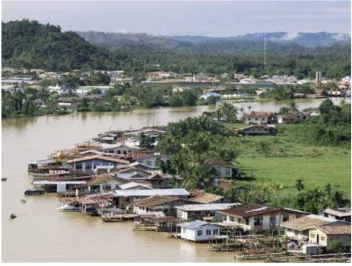
The mining activity is not the only cause of pollution in the river. Downstream the river there are human settlements (fig. 11) and, as mentioned before, the sewerage system is rudimen-tary.
Figure 11: The image is an example of human settlements across the Limbag river, in Borneo.
The organic matter coming from human waste is another se-rious problem for water quality of the river and for the negative effects that has in its fauna .
5.2 Food webs for the six sites of the river
5.2 Food webs for the six sites of the river 5 CASE STUDY I
It is photosynthesis process that helps herbivores to ingest the carbohydrates produced by a plant (primary producer). Omni-vores are species feeding at several trophic levels (in our food web they are omnivorous fish placed at intermediate position). Carnivores are considered meat-eater, their diet consists in con-sumption of other animals through predation or scavenging and in the food web are the predators placed in the top of the food web usually (in our food web are called top predator and are carnivores fish).
5.2 Food webs for the six sites of the river 5 CASE STUDY I
Names definitions of each functional group CARN carnivorous fish
PRED invertebrate predators OMNI omnivorous fish GRAZ invertebrate grazers HERB herbivorous fish
HEDE herbivore-detritivore fish SHRE invertebrate shredders
COLG invertebrate collector-gatherers COLF invertebrate collectorfilterer TERR terrestrial insects
DIAT diatoms
ALGA green and blue-green algae
POM settled and suspended coarse and fine organic particles LEAF leaf litter
HUMW human waste
FILA filamentous bacteria
Table 1: Description of functional groups in Kelian river and the names used to describe them in the food web model.
5.2 Food webs for the six sites of the river 5 CASE STUDY I
Figure 12: In site 1 the food web shows the interactions between trophic groups in the river ecosystem.
5.3 Dataset 5 CASE STUDY I
5.3 Dataset
In September 1990 (wet season) the organisms that populate the Kelian river were sampled (exactly one year before the ac-tivity of the mine). In August 1993 (dry season) after the mine has started its activity [82], then in June 1994 (dry season) and March 1995 (wet season) were done other sampling. The data comes from field data collection from 1991 until 2005 and stud-ies on fish communitstud-ies [81, 82].
The pollution on the trophic ecology in Kelian River was stud-ied by comparing food webs (on the basis of gut analysis and field and laboratory observations) at six sites paying attention to functional biodiversity of trophic groups. The species are ag-gregated in functional groups (trophic groups).
5.3 Dataset 5 CASE STUDY I
SITE 1 CARN OMNI PRED HEDE HERB GRAZ COLG COLF SHRE TERR ALGA POM DIAT LEAF
CARN 0 0 0 0 0 0 0 0 0 0 0 0 0 0
OMNI 0.111 0 0 0 0 0 0 0 0 0 0 0 0 0
PRED 0.111 0.111 0 0 0 0 0 0 0 0 0 0 0 0
HEDE 0.111 0 0 0 0 0 0 0 0 0 0 0 0 0
HERB 0.111 0 0 0 0 0 0 0 0 0 0 0 0 0
GRAZ 0.111 0.111 0.25 0 0 0 0 0 0 0 0 0 0 0
COLG 0.111 0.111 0.25 0 0 0 0 0 0 0 0 0 0 0
COLF 0.111 0.111 0.25 0 0 0 0 0 0 0 0 0 0 0
SHRE 0.111 0.111 0.25 0 0 0 0 0 0 0 0 0 0 0
TERR 0.111 0.111 0 0 0 0 0 0 0 0 0 0 0 0
ALGA 0 0.111 0 0.25 0.333 0.07 0 0 0 0 0 0 0 0 POM 0 0.111 0 0.25 0.333 0.734 1 1 0 0 0 0 0 0 DIAT 0 0.111 0 0.25 0.333 0.196 0 0 0 0 0 0 0 0
LEAF 0 0 0 0.25 0 0 0 0 1 0 0 0 0 0
Table 2: Partial feeding matrix showing interaction between predator and prey in site 1; in the columns are the predators and in the rows the preys. The matrix is estimated normalizing (the columns sum to one) the connections between trophic groups by the total intake of each receiving node.
Taking as starting point the values obtained in field samplings the individuals numbers are fitted. In case of ALGA and DIAT the fitting was harder to do.
5.4 Sites of the Kelian river 5 CASE STUDY I
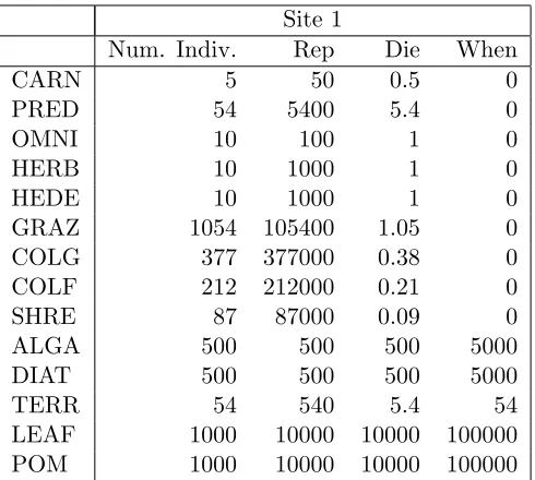
Site 1
Num. Indiv. Rep Die When
CARN 5 50 0.5 0
PRED 54 5400 5.4 0
OMNI 10 100 1 0
HERB 10 1000 1 0
HEDE 10 1000 1 0
GRAZ 1054 105400 1.05 0
COLG 377 377000 0.38 0
COLF 212 212000 0.21 0
SHRE 87 87000 0.09 0
ALGA 500 500 500 5000
DIAT 500 500 500 5000
TERR 54 540 5.4 54
LEAF 1000 10000 10000 100000
POM 1000 10000 10000 100000
Table 3: Site 1; table with the information about number of trophic groups, reproduction, death and when rates respectively.
Being a complex model with many parameters, for some data is necessary the approximation. We take a comparative ap-proach, thus the effects of making real differences in measured parameters are quantified in the context of this multi-parameter dynamical model. Finally to have a quasi-balanced behaviour in the model (no mass extinctions and exponential growths) we did some adjustments to the hypothetical values.
5.4 Sites of the Kelian river
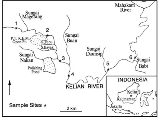
5.4 Sites of the Kelian river 5 CASE STUDY I
Figure 13: In the map river is subdivided in 6 sites in order to better study the biological communities.
The upper sites were in pristine rainforest but the river be-came increasingly polluted downstream, largely owing to sedi-mentation from alluvial gold mining activities.
Below follows the description concerning to the six sites.
• site 1 is near the pristine rainforest, upstream of the mine and Camp Prampus (miners’ houses); composition of species is mainly of diatoms and green algae
5.4 Sites of the Kelian river 5 CASE STUDY I
• site 3 is 100 m downstream of the confluence of Sungai Nakan where is construct a dam to form a polishing pond (discard water); here is where all the waste from P.E. and K.E.M. is accumulated; the flora and the fauna of the site are composed by mainly bacteria, blue green and green al-gae with the function of entrapment of fine sediments and organic matter
• site 4 situated below the P.T. K.E.M.; the banks are with sand; filamentous green and blue green algae and fungi live covering the rocks here behaving as a trap sediment and organic matter
• site 5 situated downstream of Sungai Daunsip spoiled of the vegetation; this is interest area for gold research; there is a decrease in population size and diversity of grazers, shredders and collector-filterers
• site 6 is the lowest, situated downstream of Sungai Babi and near human settlements; the water is used mainly by local people for drinking, washing and as rubbish deposit; some trophic groups are missing here or are reduced in abundance
5.5 Dynamic models 5 CASE STUDY I
and hydrological factors that influence the physical habitat, they can be used as bioindicator of water quality. These organisms were abundant in pristine site and less present downstream in correlation with the amount of fine sediment. The information that came from Yule show that pristine sites (1,2) are composed by more complex and richer fauna regarding to sites downstream (5,6). No variation in fish population is observed [70].
The different levels of human disturbance in Kelian river can be studied by comparing the structure of food webs at the 6 sites building a dynamical model, running simulation and doing sen-sitivity analyses. The analyses of food webs is necessary because the trophic interactions among aquatic organism may reflect the pollution effects.
5.5 Dynamic models
5.5 Dynamic models 5 CASE STUDY I
web). To build a dynamic model in BlenX we need information about the number of individuals, interaction rates, birth and death rates. The data about number of individuals and inter-action rates for the building of the stochastic model for Kelian river are able from field sampling [81]. We took the model in [51] as starting point to describe the stochasticity in Kelian river food webs.
The different states that an animal can be during its life-cycle are:
• eat: an animal eats the prey. In the internal process the action is presented by eat!().nil in case of the top-predator or food!().nil in case of intermediate entities.
• hunted: a prey is hunted by predator with eat?().nil action or with food?().nil action in case of the primary producers.
• duplication: intended as biological reproduction at a partic-ular rate of a functional group presented by ch(rate, dupl, duplication) action in the internal process.
• die: natural death at a particular rate of a functional group presented in the model by delay(rate).die(inf ).nil internal process.
In the model, an alternative path of duplication is possible (at specific rates depending on the species involved): if a box is put inside a new event as:
when ( Alga : : r a t e ( algaWhen ) ) new ( 1 )
5.5 Dynamic models 5 CASE STUDY I
simulator and once the simulation are finished running as out-put files are obtained res.spec file with the reactions happening during simulations, res.E.out file with the description of indi-vidual number and time steps, res.C.out and res.V.out file with variables computed in case a function is declared in .func file. In the table 4 is showed a short description of the three files compiled in order to run the simulation in BlenX.
//.PROG
[steps=120, delta=0.01]
Simulation output length−accuracy
TOP PREDATOR
let pcarn: pproc= eat!().y!().nil +
eat!().ch(rate(carnRep),dupl,duplication).nil + delay(rate(carnDie)).die(inf).nil
Process declaration of the top predator
PREY
let pherb: pproc= food!().x!().nil +
food!().ch(rate(herbRep),dupl,duplication).nil + eat?().die(inf) +
delay(rate(herbDie)).die(inf).nil
Process declaration of the prey
FOOD
let palga: pproc =
ch(rate(algaRep),dupl,duplication) +
food?().die(inf) + delay(rate(algaDie)).die(inf)
Process declaration of the producer
when (Algadup: :inf) split (Alga, Alga); Duplication event
STARTING
run 500 Alga||5 Carn||212 Colf
Initial conditions for the simulation
//.TYPES
(carn hunts, hunts pred, 0.111), (omni lifes, hunts shre, 0.111), (pred lifes, hunts graz, 0.111), (herb lifes, diat lifes, 0.333), (colf lifes, pom lifes, 1.00)
Binders of predator−prey interactions and rates
//.FUNC
let algaRep : const = 500; let algaDie : const = 500; let algaWhen : const = 5000;
Definition of the constants
5.5 Dynamic models 5 CASE STUDY I
On the top of .prog file there are some information about the time of simulation written [steps=120, delta=0.01] where steps means number of steps that the simulator will schedule and execute and delta parameter instructs the simulator to record events frequency; BASERATE : inf is used as a common basic rate for the actions which do not have an explicit rate set. At the end of the file the run command is followed by the initial condition of each functional group. The second description is about file .types which imported the predator-prey interactions followed by the feeding rates. In the beginning part of the file, all the binder’s types used in the.prog file are listed.
Finally, the .func file contains all the constants for the rates of death, reproduction and duplication of the boxes coded in the .prog file. For the producers are three parameters cited; nameRepr, nameDie and nameWhen. In file .prog the rate is used in the condition when (Food::rate(foodWhen)) new (1) in case of primary producers and this means that at a certain rate a new food is created.
In the next section we describe in more details specific internal program of the boxes in the .prog file, used to model the 6 food webs in the Kelian river. In Appendix A.1 we report the full code for the six stochastic food web models of Kelian river regarding all the sites studied in this thesis work.
5.5.1 General description of predator behaviour in BlenX
5.5 Dynamic models 5 CASE STUDY I
l e t Carn : b p r o c= #(e a t , c a r n h u n t s ) ,#( d u p l : 0 ,A) [ r e p y ? ( ) . p c a r n | p c a r n ] ;
The rep operator is used to replicate copies of the process y?().pcarn. Below follows the code that is represented by pcarn after the parallel (|) symbol:
e a t ! ( ) . y ! ( ) . n i l +
e a t ! ( ) . ch ( r a t e ( carnRep ) , dupl , d u p l i c a t i o n ) . n i l + d e l a y ( r a t e ( c a r n D i e ) ) . d i e ( i n f ) . n i l
Through the parallel processes can happen an exchange of a message from one of the subprocesses in from pcarn and the action rep y?(), generating an intra-communication. Withpcarn begins the description of the process of the predator CARN. The internal process of Carn is defined by three subprocesses linked by sum (+) operator:
l e t p c a r n : p p r o c= e a t ! ( ) . y ! ( ) . n i l +
e a t ! ( ) . ch ( r a t e ( carnRep ) , dupl , d u p l i c a t i o n ) . n i l + d e l a y ( r a t e ( c a r n D i e ) ) . d i e ( i n f ) . n i l ;
The sum operator is interpreted as a choice or, meaning that one of the three subprocesses can happen: eat!().y!().nil, just eat and restarts the internal process through the call on the y channel of the rep BlenX operator (for more details about how this operator works, we refer the reader to [14]); eat!(). ch(rate(carnRep), dupl, duplication).nil which represent the eat-ing and at a certain rate called in the model rate(carnRep) repli-cates itself; or delay(rate(carnDie)).die(inf ).nil at certain rate rate(carnDie) the predator dies. The values of the two rates rate(carnRep) and rate(carnDie) are defined in the .func file:
l e t carnRep : c o n s t = 5 0 ; l e t c a r n D i e : c o n s t = 0 . 5 ;
5.5 Dynamic models 5 CASE STUDY I
two are the binders and the third element is the affinity rate. The eat!() action needs to be coordinated with an equivalent eat?() action in a different box (in this case it will be the prey box) and the rate of this interaction is described in the .types file as follows:
( c a r n h u n t s , h u n t s h e r b , 0 . 1 1 1 )
The eat channel CARN interacts with the prey HERB with a specific affinity rate (0.111). The eat action is executed in two possible ways: 1) eat!().y!().nil sends a signal to the prey eat?().die(inf ) or in case the prey is a primary producerfood?(). die(inf ) which dies (the functional group CARN continues to live its life); 2) eat! of box CARN that sends a signal to eat? channel of box HERB.
Action change (ch) performs modification of the box interface changing the value A of the binder (dupl:0,A) in duplication (dupl:0,duplication) with a certain rate carnRep. After this is executed the box Carn will change its state into the flowing Carndup state:
l e t Carndup : b p r o c= #(e a t , c a r n h u n t s ) ,#( d u p l : 0 , d u p l i c a t i o n ) [ r e p y ? ( ) . p c a r n ] ;
and its fate is controlled by the following split event:
when ( Carndup : : i n f ) s p l i t ( Carn , Carn ) ;
Finally having all build the model in BlenX with the run command start the simulations.
5.5 Dynamic models 5 CASE STUDY I
Figure 14: The three alternative destinies of a predator are shown. The results of the two paths on the left, are (one or two) predators back in the initial state. The result of the path on the right is the disappearance of the predator box from the system. For more details about the different steps, see the description in the text.
5.5.2 General description of prey behaviour in BlenX
The box prey (e.g. HERB) is composed by a box with three binders sites (eat, food and dupl) and an internal process as follows:
l e t Herb : b p r o c = #(e a t , h u n t s h e r b ) ,#( f o o d , h e r b l i f e s ) , #(d u p l : 0 ,A)
[ r e p x ? ( ) . pherb | pherb ] ;
The internal process is composed by 4 sub-processes linked by operator sum (+):
l e t pherb : p p r o c= f o o d ! ( ) . x ! ( ) . n i l +
5.5 Dynamic models 5 CASE STUDY I
The action eat? creates an inter-communication with the corresponding eat! action of the predator (described in section 5.5.1). The action food!() of the intermediate group creates an inter-communication with the corresponding eat! action of the predator the channel food?() of the primary producer or that of another intermediate group and may have two different results: 1) a simple eating and restarting of the initial state of the box, or 2) an eating action followed by a duplication. Replication and natural mortality happen as for the predator, creation of two new boxes for the first case and deletion of a box for the second case.
5.5.3 General description of food behavior in BlenX
In our model, with the word food, we describe the primary pro-ducers. The box is composed by two binders food, dupl and an internal process, as follows:
l e t Alga : b p r o c = #(f o o d , a l g a l i f e s ) ,#( d u p l : 0 ,A) [ p a l g a ] ;
the inter-communication is executed by internal process as incoming signal and as a result of that, the box is deleted:
l e t p a l g a : p p r o c= ch ( r a t e ( algaRep ) , dupl , d u p l i c a t i o n ) + f o o d ? ( ) . d i e ( i n f ) + d e l a y ( r a t e ( a l g a D i e ) ) . d i e ( i n f ) ;
5.6 Results 5 CASE STUDY I
when ( Alga : : r a t e ( algaWhen ) ) new ( 1 )}
which means that at a certain rate algaWhen declared in file .func a new box of alga will be created.
5.6 Results
5.6 Results 5 CASE STUDY I
Figure 15: Food webs of the different sites of the Kelian river.
Some functional groups are not present in each site along the river. In sites 1 and 2 the missing species are HUMW and FILA. In sites 3 and 5 is missing only HUMW and in site 4 and 6 GRAZ, COLF, SHRE are eliminated due to pollution effects; HUMW is only in site 4 and LEAF only in site 6. Food webs show structural network differences from one site to the other. The parameters (e.g. reproduction and death rates) also show some differences from site to site. To quantify the functional ef-fects derived from these differences we perform some stochastic simulation studies and sensitivity analysis.
We developed a Python script able to control the stochastic simulator of the Beta Workbench to be able to run batches of simulation runs. After the simulations, we performed some sta-tistical analysis (as explained in Section 3.3) for all functional groups present in each specific site.
5.6 Results 5 CASE STUDY I
Figure 16: The quasi balanced system of functional groups living in site 1; each curve corresponds to a specific functional group.
Once reference simulation with the unperturbed system has been collected, we perturbed the system halving one by one the functional group. We then computed the same statistical analysis as in the previous case to compare the results. We did sensitivity analyses obtaining dynamical measurements of community importance IH(M) and IH(V).
5.6 Results 5 CASE STUDY I
IH(M)
Site 1 Site 2 Site 3 Site 4 Site 5 Site 6 CARN 0.0722 0.0714 0.0676 0.0900 0.0660 0.0859 OMNI 0.0572 0.0662 0.0696 0.0896 0.0692 0.0807
GRAZ 0.0818 0.0878 0.0838 - 0.0688
-PRED 0.0745 0.0702 0.0618 0.0590 0.0744 0.0931
SHRE 0.0736 0.0690 0.0481 - 0.0547
-COLF 0.0751 0.0689 0.0574 - 0.0557 -COLG 0.0741 0.0735 0.0751 0.0874 0.0693 0.0854 HEDE 0.0566 - 0.0560 0.0752 0.0640 0.0653 HERB 0.0707 0.0707 0.0659 0.0897 0.0574 0.0653 TERR 0.0736 0.0759 0.0481 0.0590 0.0749 0.0900 ALGA 0.0780 0.0729 0.0771 0.1078 0.0720 0.0880 POM 0.0687 0.0686 0.0820 0.0893 0.0622 0.0787 LEAF 0.0673 0.0636 0.0694 0.0789 0.0688 -DIAT 0.0765 0.0758 0.0757 0.0913 0.0759 0.0871
HUMW - - - 0.0876
FILA - - 0.0624 0.0829 0.0666 0.0929
Table 5: The table shows the community importance series IH(M) of each group in the 6 sites (in blue GRAZ which is more present in sites 2,3; decrease in site 5 and is absent in sites 4 and 6; PRED shows a decrease in the middle of the river and higher value in site 6, SHRE looking to the values we can deduce that shows sensibility to the human impact in the river).
pol-5.6 Results 5 CASE STUDY I
an adaptability to human impacts (0.0931). The invertebrate shredders (SHRE) gradually decrease in quantity from site 1 to site 3 (0.0736, 0.0690, 0.0481) and disappear in sites 4 and 6. The shredders abundance is showed to decrease from higher to lower elevations in tropical streams Peninsular Malaysia [21]. Downstream in the polluted sites (e.g. sites 3,4,5 and 6) the pri-mary producers filamentous bacteria (FILA) appear here show-ing tolerance to pollution.
The graph in figure 17 is constructed from the data in table 5. The curves show the trend of each functional group in all the sites.
Figure 17: Community importance series of the mean IH(M) of each trophic group computed for all the six sites. In the axes are represented the six sites and in the ordinate IH(M) values.
5.6 Results 5 CASE STUDY I
Figure 18: Graph shows the community importance series of the mean IH(M) for GRAZ, PRED, SHRE and FILA functional groups. In the axes are represented the six sites and in the ordinate IH(M) values.
Referring to community importance measure of dynamical variability IH(V) (table 6) GRAZ do not show the same
5.6 Results 5 CASE STUDY I
IH (V)
Site 1 Site 2 Site 3 Site 4 Site 5 Site 6 CARN 0.0355 0.0713 0.0863 0.0639 0.1294 0.1010
OMNI 0.0524 0.0595 0.0642 0.1271 0.0744 0.1463
GRAZ 0.0661 0.0777 0.0642 - 0.0472 -PRED 0.0666 0.0800 0.0724 0.0759 0.0509 0.0761 COLF 0.0593 0.0570 0.0726 - 0.0664 -COLG 0.0723 0.0801 0.0472 0.0797 0.0768 0.0650 HEDE 0.0813 0.0575 0.0579 0.1283 0.0616 0.0672 HERB 0.0755 0.0772 0.0521 0.0755 0.0632 0.0807 SHRE 0.0663 0.0784 0.0654 - 0.0496
-ALGA 0.0860 0.0653 0.0789 0.0879 0.0666 0.0611
DIAT 0.0903 0.0516 0.0473 0.0666 0.0769 0.1110
LEAF 0,0915 0,0741 0.0746 0.0754 0.0586
-POM 0.0821 0.0763 0.0702 0.0813 0.0512 0.0690
TERR 0.0748 0.0940 0.0654 0.0759 0.0763 0.0556
HUMW - - - 0.0543
FILA - - 0.0813 0.0625 0.0511 0.1126
Table 6: The table shows IH(V) index which quantifies community impor-tance based on the influence of dynamical variability of each group in the 6 sites (in blue OMNI which present an increase in abundance in all the sites especially in site 6, LEAF, DIAT, ALGA, POM which decrease in abundance from upstream to downstream the river).
In figure 19 the graph shows the results curves obtained from the IH(V) index measure, showed in table 6, for all the
5.6 Results 5 CASE STUDY I
Figure 19: Community importance series of the variance (IH(V)) of each trophic group computed for the six sites. In the axes are represented the six sites and in the ordinate IH(V) values.
The primary producers (LEAF, DIAT, ALGA, POM) show decrease in abundance from upstream to downstream the river and especially in sites 2 and 6 where the human impacts are stronger. IH(V) index suggests that disturbing the primary
5.7 Conclusion 5 CASE STUDY I
Figure 20: Through the community importance series of the variance IH(V) in the graph we can observe how the curves of primary producers (LEAF, DIAT, ALGA, POM) decrease in abundance; the omnivores (OMNI) increase in abundance. In the axes are represented the six sites and in the ordinate IH(V) values.
5.7 Conclusion
The mine activity and human settlements with their discarded materials have affected trophic interactions of the food webs of the river with consequences for the benthic flora and filter-feeding invertebrates.
5.7 Conclusion 5 CASE STUDY I
Using dynamical simulations we aim to analyse the functional diversity of ecosystem at the level of functional groups. From our results we can infer that the invertebrate shredders (SHRE) are indicators of human impact on the river. The role of shred-ders in food web development is very important [35], because breaking down leaves into smaller particles they supply food for other organisms as collector gatherers and filters. In sites that are located downstream along the river, the vegetation is more sparse, so there is a decrease supply in leaf litter. The primary producers as diatoms (DIAT), algae (ALGA), filamentous bac-teria (FILA) disappear downstream likely because of the excess of sediments that is the consequence of mine activity and of the presence of human waste. This effect can be mostly seen in site 6, which is the most polluted site. The grazers (GRAZ) are less important downstream, since other groups as fish omnivores (OMNI) and carnivores (CARN) tolerate better the human in-fluence on the river and their variety is less strong than the one of invertebrate groups.
6 CASE STUDY II
6
Case study II
6.1 Fishing by FADs on tunas, Gulf of Guinea
6.1 Fishing by FADs on tunas, Gulf of Guinea 6 CASE STUDY II
Figure 21: Map of Gulf of Guinea
consid-6.1 Fishing by FADs on tunas, Gulf of Guinea 6 CASE STUDY II
Figure 22: The image represents a drawing of an adult skipjack tuna ( Kat-suwonus pelamis).
The fishing activity on skipjack is done using almost exclu-sively surface gears throughout the Atlantic, mainly by baitboat and purse seine vessels and a small numbers of them are conse-quence of incidental longline catches.
Figure 23: The map is representation of geographical distribution of skipjack catches by principal gears (ICCAT Secretariat [44]).
aggre-6.1 Fishing by FADs on tunas, Gulf of Guinea 6 CASE STUDY II
gating devices (FADs) [23, 12]. Tuna stocks catches represents nearly half of all principal market. Nowadays fishing opera-tions on tuna schools associated with drifting FADs became widespread in the Eastern Tropical Atlantic [80]. In the early 1990s, fishing operations on tuna schools associated with drift-ing FADs became widespread in the Eastern Tropical Atlantic [80]. From ICCAT [44] we can read that the percentage of skip-jack tuna catched under FADs reaches 90%, with only a small 10% catched using other methods. The ICCAT report is fo-cused especially on South Gulf of Guinea area more important for fishing made by the use of drifting FADs (see figure 24).
Figure 24: Skipjack tuna catches in free schools and under FADS, 1991-2006.