Wireless Sensor Node Localization Algorithm Based on Particle Swarm Optimization and Quantum Neural Network

Wireless Sensor Node Localization Algorithm Based on

Particle Swarm Optimization and Quantum Neural

Network

https://doi.org/10.3991/ijoe.v14i10.9314

Yulong Liu(*_{), Xiaoming Yu, Yuhua Hao}

Yancheng Institute of Technology, Yancheng, China [email protected]

Abstract—Aiming at the problem of node localization in wireless sensor net-works, a location algorithm for optimizing distance vector hopping (DV-hop) by constructing a quantum neural network model based on particle swarm optimiza-tion (PSO) is proposed. According to the average distance obtained by the tradi-tional DV-HOP and the distance from the measured nodes, the quantum neural network model is constructed, and the average distance is trained by the particle swarm optimization algorithm which would shorten the training time of the tra-ditional artificial neural network and accelerate the convergence speed. By using the proposed model, the optimal mean value is obtained, and the optimization of the DV-HOP algorithm is realized. The simulation results show that compared with the traditional DV-HOP algorithm, the proposed algorithm can reduce the positioning error by about 20%, and the positioning accuracy is significantly im-proved.

Keywords—wireless sensor networks, quantum neural network, particle swarm optimization, DV-HOP algorithm

1

Introduction

In recent years, the research results of wireless sensor networks (WSNs) have been widely used in environmental detection, target tracking, military and other fields [1]. With the deep integration of WSNs theory research and practical application [2-4], the current research on WSNs is mainly in three aspects: the energy consumption, node deployment and node location of network nodes. The research of node location is the premise of sensor networks in many fields [5].

What is worth mentioning here is that we mainly focus on range-free localization algorithm, especially DV-HOP. The traditional DV-HOP algorithm mainly relies on the estimation of the average hop distance in the process of WSNs node localization. The misbehavior nodes in the network will result in the unreasonable hops information obtained, so that there is a large error in the average single-hop distance obtained from the hop information. As a result, the accuracy and efficiency of WSNs node localization decrease sharply, which makes the positioning process is fuzzy and uncertain.

Therefore, we use particle swarm optimization (PSO) algorithm as the learning mechanism of quantum neural network (QNN) [9], and propose a PSO-QNN localiza-tion algorithm for WSNs. By combining the two algorithms, a node localizalocaliza-tion model with short learning time, fast convergence speed and high precision is constructed, and after training, quantum neural network obtains the best initialization weights and thresholds. As a result, when the model is applied to DV-HOP algorithm, a better aver-age hop distance is obtained, thus improving the positioning accuracy of nodes. Be-sides, simulation results show that the algorithm has greatly improved the positioning accuracy and efficiency.

2

DV-HOP Algorithm

Figure 1 is a concrete indication of the principle of hop distance.

Fig. 1. The principle of hop distance

In Figure 1, A is the anchor node, and the communication radius is r, the I, II and III regions are the first, second and third hop restricted regions of anchor node A.

(1)

Where (xi, yi)(xj, yj) are the position coordinates of node i and node j respectively. hij

is the number of hops between anchor node i and anchor node j. Then, the average hop distance as the correction value is broadcast throughout the whole WSNs. When the first correction value is received, the pending node will save it and then no longer re-ceive other correction values. According to the correction value, convert the minimum hop count between the node and anchor node to the distance of them; 3) When the location node gets three or more than three anchor nodes, the nodes to be located can be obtained by three or multilateral measurements.

3

DV-HOP Algorithm Based on PSO-QNN

3.1 Quantum neural network

The back propagation (BP) neural network consists of three layers: input layer, hid-den layer and output layer. In BP model, input layer LA, output layer LC and hidhid-den layer LB are composed of m, n and p nodes respectively. Moreover, the nodes of the same layer are not connected, and the adjacent layer nodes are all interconnected.

The output of the hidden layer LB of traditional BP neural network can be expressed as follows:

(2)

The output of the output layer LC can be expressed as follows:

(3)

where the corresponding relationship 𝑓𝑓 is function 𝑆𝑆𝑆𝑆𝑆𝑆𝑆𝑆𝑆𝑆𝑆𝑆𝑆𝑆 (it is also called S growth curve), that is, 𝑓𝑓(𝑥𝑥) = (1 + 𝑒𝑒01_{); 𝑋𝑋 is the input of the neural network, the}

neu-ron of the input layer is represented by 𝑎𝑎4, in the same way, the hidden layer is 𝑏𝑏6, and

the output layer is 𝑐𝑐8. Besides, 𝑊𝑊46 is the connection weight between the input layer

neuron and the hidden layer neuron; 𝑉𝑉68 is the connection weight between the hidden

layer neuron and the output layer neuron; 𝜃𝜃 is the threshold of the hidden layer, and 𝜑𝜑

is the threshold of the output layer.

For quantum neural network model [11-14], the multiple Sigmoid functions are su-perimposed, and a hidden layer neuron can represent a number of orders of magnitude, thus constructing an incentive function of a sandwich-like structure, it makes the fuzz-iness of the network increase substantially. Now, the hidden layer output can be ex-pressed as follows:

j i h

y y x x d

j i ij j

i i j i j

HOP

DV ¹

-+ -=

å

å

¹ ¹

- ,

) ( )

( 2 2

p r

X W f

b T

r= ( -

q

n

j

B

V

f

c

(4)

Where 𝑛𝑛D is the number of quantum intervals, which is the same as the number of

faults. Meanwhile, 𝛼𝛼F is a steepness factor, 𝜃𝜃6 is a quantum interval.

The gradient neural network algorithm is still used in the training algorithm of lay-ered excitation function. In the training process, the updated contents include the con-nection weights between different layers of neurons and the quantum spacing between neurons in the hidden layer.

Here, the updating of connection weights is no different from that of BP neural net-work. And the quantum interval algorithm for hidden layer neurons is updated.

For the pattern class vector 𝐶𝐶F (m is the number of pattern class, that is, the number

of neurons in the input layer), so the output variables of the j neurons in the hidden layer can be expressed as follows:

(5)

(6)

where 𝑂𝑂8,J is the output of the j neurons in the hidden layer when the input vector is

𝑥𝑥J.

By minimizing the total class variance 𝛿𝛿8L, the renewal equation of the hidden layer

quantum interval 𝜃𝜃86 can be obtained, and the 𝛾𝛾 quantum interval of the j neurons in the

hidden layer can be expressed as follows:

(7)

Where 𝜂𝜂 is the learning rate, and 𝛼𝛼F is the steepness factor.

3.2 Particle swarm optimization algorithm

For particle swarm optimization algorithm, suppose that there is a n dimension target search space composed of m particles, then the position of the p particle in d dimension space is

(8)

Flight speed can be expressed as follows:

(9)

The fitness value is expressed as follows: p r

X W f n

b ns

r

T m s

r 1 [ ( )], ,12,3, , 1

! =

-=

å

=

g

q a

å

Î

-=

m kC

x jm jk

m

j, 2 (O, O,)2

s

å

Î

=

m k C

x jk

m m

j, _C1 O.

O

å å

= Î

-=

D s

m k

n

m x C

jk jm jk jm s

m _{h h v v}

n 1

j ( )( )

g g g _ha

q

[

]

p , , , , , ,12, ,

L = _{1 2 3}! = !

[

]

p , , , , , ,12, ,

(10)

The algorithm has two extremes: the best solution 𝑝𝑝𝑏𝑏𝑒𝑒𝑝𝑝𝑝𝑝 found by each particle it-self; the best location 𝑆𝑆𝑏𝑏𝑒𝑒𝑝𝑝𝑝𝑝 found by the whole particle swarm. The position and ve-locity of particle p in the d dimensional space are updated according to the following iterative equation:

(11)

(12) where 𝑉𝑉RSJ represents the flight speed of the first 𝑘𝑘 iteration of the 𝑝𝑝 particle in the d

dimension space; then 𝐿𝐿JRS is the position of the 𝑝𝑝 particle in the d dimensional space

for the 𝑘𝑘 iteration; 𝑟𝑟𝑎𝑎𝑛𝑛𝑆𝑆() is a random number between [0, 1]; 𝑐𝑐W and 𝑐𝑐L are both

learn-ing factors. The particle search will stop at the best location or the maximum number of iterations. The PSO algorithm flow is shown in Figure 2.

Fig. 2. Flow chart of particle swarm optimization algorithm

3.3 Algorithm implementation steps

Assuming that the number of anchor nodes is P, and the number of nodes to be po-sitioned is M. Then the whole WSNs node localization steps are as follows:

1. Establish the PSO-QNN empirical model and use the prearranged anchor node to perceive the environment. Through two sets of data (the actual distance 𝐷𝐷{𝑆𝑆48, i ≠ j}

between the anchor node and other anchor nodes and the average distance

𝐷𝐷∗_{𝑆𝑆

48∗, i ≠ j} between the anchor node and other anchor nodes), PSO can train QNN

and optimize the initial weight and quantum interval of QNN. )

( fitness_p = f L_p

) (

() rand )

( ()

Vpdk+1=Vpdk +c1´rand ´ pbestkpd -Lkpd +c2´ ´ gbestpdk -Lkpd

1

1 +

+

₌

₊

pd k pd k

pd

L

V

2. PSO algorithm has a very strong searching ability, which can obtain the global opti-mal solution for each particle.

3. After establishing the model, the anchor nodes and the nodes to be located are dis-tributed in WSNs. Each anchor node regularly broadcasts its own related parameters in the WSNs, including the node coordinates and the parameters of the quantum neural network. All nodes get the minimum hop count to the anchor node through the distance vector exchange protocol.

4. According to the location information and hop count of each anchor node recorded to other anchor nodes, the average distance per hop is calculated by Eq. (1). 5. The average hop distance 𝑆𝑆ccccccccccc^_0`ab obtained in step (4) is used as the input of the

PSO-QNN model, then the optimized distance value 𝑆𝑆cccccccccccc,i = 1,2,3,…𝑞𝑞bda0eff can

be obtained at the output of the model. 𝑞𝑞 is the number of selected anchor nodes. 6. According to the average hop distance 𝑆𝑆bda0eff, it will be broadcast as a correction

value in the whole WSNs.

7. When the first correction value is received and saved by the location node, it is for-warded to the adjacent node, and the location node calculates the hop distance to each anchor node according to the corrected value and the recorded hops infor-mation.

8. When the location node gets three or more than three anchor nodes, the nodes to be located can be obtained by three or multilateral measurements.

3.4 Algorithm specific description

The initialization of PSO algorithm is the process of finding the optimal solution through a continuous population iteration of a group of randomly distributed particles. By comparing the optimal solution of the new generation with the previous generation, the optimal value is updated, such as Eq. (11) and Eq. (12). Matlab is used to build the simulation environment of the logarithmic - constant distribution model. According to the measured node distance 𝐷𝐷{𝑆𝑆48, i ≠ j} and the average distance 𝐷𝐷∗{𝑆𝑆48∗, i ≠ j}, the

quantum neural network model is constructed based on the traditional DV-HOP algo-rithm. In this way, the average distance 𝐷𝐷∗ _{is trained by the PSO algorithm, thus the}

better average value is obtained.

First of all, we should select corresponding data to learn and train QNN, so as to form a practical model applied to WSNs positioning. We trained the parameters of QNN through PSO. The parameters for QNN to be trained are the 𝑆𝑆 × 𝑝𝑝 parameter 𝜃𝜃

Assuming that the number of training samples is N, and the MSE of the network is expressed as follows:

(13)

Where the tij in the formula is the expected output value of sample i on the j output

terminal.

The coordinates of the nodes to be positioned in the three side or the multilateral measurement method are (x, y) . The coordinates of the anchor nodes are

(xW, yW), (xL, yL), (xo, yo), … , (xp, yp), in this way, the distance from the location node

to the anchor node can be expressed as dW, dL, do, … , dp, respectively.

(14)

Especially, let

Here, , according to Eq. (14), it satisfies the relationship 𝐴𝐴𝑋𝑋 = 𝐵𝐵. By

sim-plification, the following relationship can be obtained

(15)

Accordingly, the position coordinates of the nodes to be located can be obtained by the Eq. (15).

4

Simulation Results

The experiment is carried out in Matlab7.0 simulation environment, which is specif-ically configured as Intel (R) Core (TM) i3-2370M CPU, 2.40GHz, and 4GB memory

åå

platform. In the simulation experiment, a node location detection area of

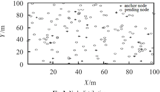
100𝑆𝑆 × 100𝑆𝑆 is constructed. More specifically, the communication radius of the node r is set to 25m, which contains 150 sensor nodes and is deployed randomly. In the PSO algorithm, the number of initialization of the particle swarm m is set to 40, the maxi-mum iteration number Q is set to100, 𝑐𝑐W and 𝑐𝑐L are the learning factor, their value both

are 1.8. Additionally, the anchor node and the location node are distributed as Figure 3.

Fig. 3. Node distribution

4.1 The number of anchor nodes’ influence on positioning error

The nodes are located according to the implementation steps of the proposed algo-rithm, and then the average positioning error is obtained based on the simulation results [15-16]. The average location error is defined as

(16)

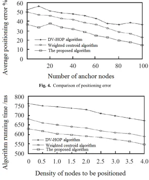
From Figure 4, we can see that in the same environment, the location error of the algorithm is much lower than that of the traditional DV-HOP algorithm. Additionally, the weighted centroid algorithm is selected as the contrast algorithm. It can be seen that the average positioning error of the three algorithms decreases with the increase of an-chor nodes. As a consequence, the average location error of the proposed algorithm is about 26%, in comparison, the weighted centroid algorithm is about 38% and the tradi-tional DV-HOP algorithm is about 48%. Thus this algorithm reduces the average posi-tioning error by about 20% compared with the traditional DV-HOP algorithm.

Due to the large error in the process of hopping to distance, the algorithm requires the nodes to be positioned should have a high density in the implementation process. The simulation results are shown in Figure 5, with the increase of the density of the nodes to be located, the duration of the 3 algorithms is reduced. Accordingly, the time required in this algorithm is reduced by about 100ms compared with the traditional DV-HOP algorithm.

% 100 ) ( ) (

1

2 2

´ -+ -=

å

Mr y y x x e

M

i i i

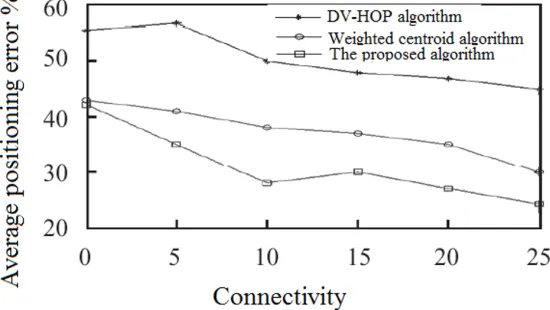
Information can be transmitted directly between nodes by using DV-HOP algorithm. Actually, connectivity mainly reflects the relationship between the number of anchor nodes and the radius of communication. In view of that, the experiment compares the positioning error by analyzing the change of connectivity. From Figure 6, we can see that with the increase of connectivity, the average positioning error of the three algo-rithms is decreasing in general. Therefore, under the same connectivity, the positioning error of the proposed algorithm is the smallest.

Fig. 4. Comparison of positioning error

Fig. 6. The influence of different connectivity on the average positioning error

5

Conclusions

In view of the problem that DV-HOP algorithm is easily affected by the external environment factors during the location of WSNs nodes, PSO-QNN algorithm is pro-posed. Compared with the traditional BP neural network [17], QNN accelerates the convergence speed of the algorithm, and more importantly, it reduces its fuzziness. Furthermore, by using the PSO algorithm as the learning algorithm of QNN, we con-structed the PSO-QNN network model, and the DV-HOP algorithm is further im-proved. The data obtained are analyzed through simulation experiments from three as-pects, and the results show that the positioning accuracy of this algorithm has been greatly improved, up to about 20%, which proves the effectiveness of the algorithm in the node location.

6

References

[1]Fu, L.H. (2010). Method to Decrease Noise in Speech Based on Improved Quantum Neural Networks. Information and Control, 39(4): 466-471.

[2]Gai, H.C., Zhang, X.F., Jiang, Z.T. (2010). Face recognition technology based On Quan-tum Neural Networks. Computer Engineering and Applications 2010; 46(8):187-189. [3]Li, P., Liao, B., Luo, J., Wu, D. (2008). Localization Method in Mobile Wireless Sen-sor

Networks. Journal of Chinese Computer Systems, 29(11): 2051-2054.

[4]Litvintseva, L.V., Ul'Yanov, S.V. (2009). Intelligent control systems. I. Quantum computing and self-organization algorithm. Journal of Computer & Systems Sciences International, 48(6):946-984. https://doi.org/10.1134/S1064230709060112

[5]Ma, Z., Sun, Y., Mei, T. (2004). Survey On wireless sensors network. Journal of China In-stitute of Communication, 25(4): 114-124.

[6]Paula, T., Bernardos, A.M., Casar, J.R. (2011). Weighted Least Squares Techniques for Im-proved Received Signal Strength Based Localization. Sensors, 11(9): 8569-8592.

[7] Shi, H., Wang, W. (2010). Game theory for wireless sensor networks: A survey. Sen-sors, 12(7): 9055-9097. https://doi.org/10.3390/s120709055

[8] Shi, W.R., Jia, C.J., Liang, H.H. (2011). An Improved DV-Hop Localization Algorithm for Wireless Sensor Networks. Chinese Journal of Sensors and Actuators, 24(1): 83-87. [9] Shi, X.W., Zhang, H.Q., Deng, G.H. (2012). Research on Indoor Location Algorithm based

on Distance-loss Model Using Back Propagation Neural Network. Computer Measurement & Control, 20(7): 1944-1947.

[10] Sun, G., Bin, S. (2017). Router-level internet topology evolution model based on mul-ti-subnet composited complex network model. Journal of Internet Technology, 18(6): 1275-1283.

[11] Sun, G., Bin, S. (2018). A new opinion leaders detecting algorithm in multi-relationship online social networks. Multimedia Tools & Applications, 77(4): 4295–4307.

https://doi.org/10.1007/s11042-017-4766-y

[12] Tang, W., Zhou, L. (2015). An improved APIT localization algorithm based on trian-gle-circumcircle cover. Chinese Journal of Sensors & Actuators, 28 (1): 121-125.

[13] Tao, Z.Y., Wei, Q., Liu, Y. (2014). Improved DV-Hop localization algorithm based on more power auxiliary anchor nodes. Computer Engineering and Applications, 50(21): 121-124. [14] Wang, Y., Shi, H. (2012). Improved DV-Hop Localization Algorithm for Wireless Sensor

Network. Computer Engineering, 38(7):66-69.

[15] Zhang, P., Mao, W., Xu, J. (2015). A secure ire localization algorithm for WSNs based on iterative vote. Transducer and Microsystem Technology, 34(12):118-120.

[16] Zhang, Y.P., Chen, L., Hao, H. (2013). An Improved Training Algorithm for Quantum Neu-ral Networks. Journal of Electronics & Information technology, 35(7):1630-1635.

https://doi.org/10.3724/SP.J.1146.2012.01417

[17] Wang, T.C., Xie, Y.Z., Yan, H. (2016). Research of multi sensor information fusion tech-nology based on extension neural network. Mathematical Modelling of Engineer-ing Prob-lems, 3(3): 129-134. https://doi.org/10.18280/mmep.030303

7

Authors

Yulong Liu has a Master's degree and is an associate professor at the School of Mathematics and Physics, Yancheng Institute of Technology, Yancheng 224051, China, he is mainly engaged in teaching basic physics and researching the properties of nanomaterials.

Xiaoming Yu is a PhD student and is an associate professor at the School of Math-ematics and Physics, Yancheng Institute of Technology, Yancheng 224051, China, he is mainly engaged in basic physics teaching and computational physics and other re-search work.

Yuhua Hao is an associate professor at the School of Mathematics and Physics, Yancheng Institute of Technology, Yancheng 224051, China, he is mainly engaged in basic physics teaching and applied physics research.