Abstract— In reality, the heterogeneous wireless sensor networks (HWSN) are deployed in Three-Dimensional (3D) environment. However, most studies about this type of network consider that the distribution of these nodes is done in Two-Dimensional (2D) environment within reason to simplify the calculation analysis. Unfortunately, the lifetime and throughput in the 3D environment of HWSN decreases considerably compared to 2D model. These two performance indicators can’t be neglected in some applications. In this paper, we applied the 3D architecture in SEP protocol and we show by computer simulation how this 2D approximation is not reasonable. In fact, this approach does not reflect the real energy consumption in the network nodes because the discard between the lifetimes of 3D-SEP and 2D-3D-SEP decrease by an important rate.
Index Terms— Wireless sensor networks, SEP protocol, Energy-efficiency, 2D and 3D HWSN, Network lifetime.
I. INTRODUCTION
ECENTLY, the development of the embedded system
and wireless communication technologies have enabled the appearance of the tiny nodes called wireless sensor network WSN that are equipped with sensing unit, processing unit and communication unit [1]. All these units are usually powered by a single battery, whose replacement is generally impossible. These nodes are deployed in the large area in the goal to monitor this field and send the detection event toward the base station. Energy consumption in this network is dissipated up in three essential functionalities of WSNs such as detection, data aggregation, and the communication. According to literature [2], this last operation consumes more energy compared to the others. Therefore, to prolong the lifetime of these nodes, the direct transmissions must be avoided [3]. To reduce long distance transmissions, the simple idea is to divide network into small regions of nodes called clusters which each of them is managed by one node named cluster head CH [4]. As it collects the data from member nodes and sends them toward base station or through otherMostafa Baghouri, Abderrahmane Hajraoui, Saad Chakkor are with the Department of Physics, Communication and detection systems laboratory, Faculty of Sciences, University of Abdelmalek Essaâdi, Tetouan,
Morocco (e-mail: [email protected], [email protected],
[email protected], respectively).
CHs by using multi-hop communication, its energy is depleted very quickly. Some researchers propose to select these CHs periodically while based on a threshold [5] [6] [7] [8]. All of these protocols and others assume that all nodes of the network have the same energy level. This means that the network is homogeneous. However, sensor nodes don’t have the possibility to maintain energy in the same way during the cycles, the fact that they don’t have the same position in the network [9]. This means that the network is heterogeneous. In this context, many researchers call for consider, first of all, that the network is heterogeneous in the goal to converge into the reality and minimize the estimations [10][11].
Generally, the HWSNs have many applications such as underwater sensor network, Ocean column monitoring, monitoring railway tunnels, and underground tunnels in the mine. In these applications, the nodes are deployed in three-dimensional environment (3D) which has been modeled by the researchers in two-dimensional space (2D). However, this assumption is invalid in the reality when the height of the network is no negligible [12].
In this paper, we applied the 3D architecture in Stable Election Protocol (SEP) [9] which is one of interesting protocol under heterogeneous environment and we show by computer simulation how this 2D approximation is not reasonable.
The rest of the paper organization is done as follows: Section II summarizes the related work. Problem Statement is provided in section III. Three-dimensional stable election protocol for wireless sensor network models has introduced in section IV. The Simulation results are carried out in section V. Finally we conclude our research work and give some perspectives in section VI.
II. RELATED WORK
In the last years, the researchers focalize their ideas around the clustered heterogeneous WSN with the goal to prolong the lifetime of these tiny nodes. G. Smaragdakis et al. have proposed Stable Election Protocol for clustered heterogeneous wireless sensor networks (SEP) [9] to stabilize in the most, the heterogeneous two-level hierarchical network by choosing each node its own election probability. M. Baghouri et al. have improving this protocol by using the fuzzy logic approach by computing the choice that each node to become cluster head
Three-Dimensional Stable Election Protocol for
Clustered Heterogeneous Wireless Sensor
Network
M. Baghouri, A. Hajraoui and S. Chakkor
[13]. SEP-FL is based on two criteria: the distance from the base station and the residual energy level of each node type. The SEP-FL increases the stability period and decreases the instability of the sensor network as compared with LEACH (Low Energy Adaptive Clustering Hierarchy) and SEP. This protocol provides longer interval of stability for large values of additional energy brought by advanced nodes. M. Baghouri et al. prove by simulation that 2D environment approximation is not valid in the some applications [14]. They compared 3D architecture in LEACH protocol with 2D and show that the lifetime and throughput of the network decrease considerably witch can’t neglect them in the some applications. Xi Zhang et al. [15] have described mechanism of three dimensional clustering to maximize the lifetime of network by considering the minimum coverage rate constraint. This paper proposed new protocol by enhancing the LEACH protocol using the basic assumption of SEP protocol in which advanced nodes have more energy than initial node. Attarzadehet et al. [16] have describe the method of clustering called three dimensional clustering which resolve the restriction of two dimensional clustering by providing the different surface for review space. This paper define the three different levels, first for sink node which is at highest point, second level is first cluster heads and third level is for different number of nodes which are active. This method is used to achieve better performance of network. Some researches consider that sensor coverage is a primary factor for wireless sensor network deployments. Indeed, X. Bai et al and S. Kumar et al consider 2D ideal plane [17] [18], contrariwise, C. F. Huang et al, M. Watfa et al, use 3D space models [19] [20]. Linghe Kong et al. [21] demonstrate that the coverage of sensor networks in real environments is 3D. In this paper, the authors describe the Tungurahua volcano monitoring project and resolve the coverage dead zone problem, by replacing 2D surface coverage model by 3D sensor network deployments. Thus, they establish the new links for coverage these dead zones.
Based on the analysis above, we find that few works on 3D deployment have been studied for HWSNs. Driven by this observation; we will show by simulation that these assumptions and approximations to 2D surface are not reasonable in some applications of HWSN.
III. PROBLEM STATEMENT
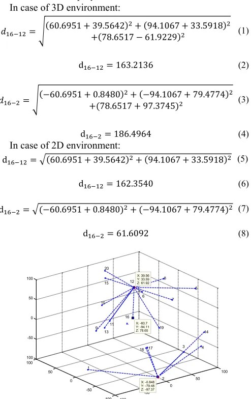
Let us consider a set of 20 nodes deployed randomly in the 3D space shown in Figure 1. According to the clustering-based topology, each CH aggregated the data from the member nodes and then transmits them to the base station via a multi-hop communication. Let us consider likewise a set of same nodes deployed in 2D environment Figure2. The nodes undergo the same process of electing the cluster heads than the 3D terrain. By analysis of these figures, we remark that some nodes which are attached with one cluster head in 3D space, are join other cluster head in 2D environment. Indeed, node number 16 join cluster head number 12 in 3D architecture, however, it join cluster head number 2 in the 2D environment.
To clearly understand this error, let us calculated the
distance between these two nodes to their cluster heads in the different case of deployment:
In case of 3D environment:
𝑑16−12= √(60.6951 + 39.5642)
2+ (94.1067 + 33.5918)2
+(78.6517 − 61.9229)2 (1)
d16−12= 163.2136 (2)
𝑑16−2= √(−60.6951 + 0.8480)
2+ (−94.1067 + 79.4774)2
+(78.6517 + 97.3745)2 (3)
d16−2= 186.4964 (4)
In case of 2D environment:
d16−12= √(60.6951 + 39.5642)2+ (94.1067 + 33.5918)2 (5)
d16−12= 162.3540 (6)
d16−2= √(−60.6951 + 0.8480)2+ (−94.1067 + 79.4774)2 (7)
d16−2= 61.6092 (8)
Figure 1:Three-dimensional Wireless Sensor Network model with 20 nodes
Figure 2:Two-dimensional Wireless Sensor Network model with same configuration
From this example, it is clear that node 16 attached to the cluster head number 12 in the 3D environment and chooses the cluster head number 2 in the 2D architecture. Therefore it is difficult to model the network in 2D environment because a
-100 -50
0 50
100
-100 -50 0 50 100 -100 -50 0 50 100
14
4 5
3 7 8
2 19
17 6
X: -0.848 Y: -79.48 Z: -97.37
18
X: 39.56 Y: 33.59 Z: 61.92
X: -60.7 Y: -94.11 Z: 78.65
12
16 11 20
13 15
10
9
1
-100 -80 -60 -40 -20 0 20 40 60 80 100 -100
-80 -60 -40 -20 0 20 40 60 80 100
1
4 5
7 11
14 18
19 20
X: 39.56 Y: 33.59
X: -60.7
Y: -94.11 X: -0.848
Y: -79.48
2
3 6
8
9 10
12 13
15
16
node attached with a cluster in 3D space will not necessarily be tied with the same cluster in 2D architecture since the distance is not the same.
Generally, the fact that the distance between the nodes is not properly calculated accurately, influence on the clusters formation in the network and consequently it leads to a bad clustering and therefore a bad energy consumption management.
In this paper, we demonstrate by simulation that the modeling of the network by 2D environment is not realistic. Indeed we applied the 3D model in SEP and we show that this model is more stable than the 2D model.
IV. THREE-DIMENSIONAL STABLE ELECTION PROTOCOL FOR
WIRELESS SENSOR NETWORK MODELS A. Network Model
To simplify model construction, we consider the following basic assumptions:
1.
All nodes are deployed randomly and uniform within a square 3D rectangular field of aria 𝐴 = 𝑀 × 𝑀 × 𝑀2.
The base station is located in the center of the sensornetwork
3.
The nodes are considered heterogeneous with two levels (advanced and normal nodes)4.
The communication between nodes is making by using variable power levels.5.
Each node calculates the approximate 3D distance to other node base on the received signal strength.6.
Each node is known by an identifier (ID) that localized (see Figure 3)Figure 3:Three-dimensional Wireless Sensor Network model
B. Energy Model
To modelize the energy dissipation in each node of WSN, we consider a simple radio energy dissipation model illustrated in Figure4:
Figure 4:Three-dimensional Wireless Sensor Network model
Where the transmitter dissipates energy in two modules: the electronics radio module for transmitting and amplifying module and the receiver signals dissipates energy in the radio electronics module for receiving signals. Using this radio model, to transmit l-bit messages at distance d the radio expends:
𝐸𝑇𝑥(𝑙, 𝑑) = 𝐸𝑇𝑥−𝑒𝑙𝑒𝑐(𝑙) + 𝐸𝑇𝑥−𝑎𝑚𝑝(𝑙, 𝑑) (9)
Where ETx−elec(l) is the energy dissipating for running the
circuit electronics to transmit l-bits of data:
𝐸𝑇𝑥−𝑒𝑙𝑒𝑐(𝑙) = 𝑙𝐸𝑒𝑙𝑒𝑐 (10)
And ETx−amp(l, d) is the energy dissipated by the
amplifying module which depend by the distance between transmitter and receiver and can be calculated as fellow:
𝐸𝑇𝑥−𝑎𝑚𝑝(𝑙, 𝑑) = {
𝑙𝜖𝑓𝑠𝑑2, 𝑤ℎ𝑒𝑛 𝑑 < 𝑑0
𝑙𝜖𝑚𝑝𝑑4, 𝑤ℎ𝑒𝑛 𝑑 ≥ 𝑑0 (11)
Where 𝜖𝑓𝑠 is amount of energy consumption for free space
and 𝜖𝑚𝑝 is amount of energy consumption for multipath
fading. dois the distance threshold for swapping amplification models, which can be calculated as:
𝑑𝑜= √
𝜖𝑓𝑠
𝜖𝑚𝑝 (12)
To receive an 𝑙 − 𝑏𝑖𝑡𝑠 messages the receiver circuit can expends:
𝐸𝑅𝑥(𝑙) = 𝑙𝐸𝑒𝑙𝑒𝑐 (13)
To aggregate N data signals of length l − bits, the energy consumption was calculated as:
𝐸𝐷𝐴−𝑒𝑥𝑝𝑒𝑛𝑑(𝑙) = 𝑙𝑁𝐸𝐷𝐴 (14)
C. Optimal number of cluster
We assume there are N nodes distributed uniformly in
𝑀 × 𝑀 × 𝑀 3D region. If there are c clusters, there are on
average 𝑁/𝑐 nodes per cluster. Each cluster-head dissipates energy receiving signals from the nodes and transmitting the aggregate signal to the base station. Therefore, the energy 0
20 40
60 80
100
0 20 40 60 80 100
0 20 40 60 80 100
z
(m
)
3D Wireless Sensor Network model
x(m)
y(m)
Sin k
d
𝐸𝑇𝑥(𝑙, 𝑑)
𝐸𝑇𝑥−𝑒𝑙𝑒𝑐(𝑙) 𝐸𝑇𝑥−𝑎𝑚𝑝(𝑙, 𝑑)
TX Amplifier Transmit
Electronics
l bits of packets
𝐸𝑅𝑥(𝑙)
𝐸𝑅𝑥(𝑙)
Receiver Electronics
dissipated in the cluster-head node during a single frame is:
𝐸𝐶𝐻 = 𝑙
𝑁
𝑐𝐸𝑒𝑙𝑒𝑐+ 𝑙
𝑁
𝑐𝐸𝐷𝐴+ 𝑙𝜖𝑚𝑝𝑑𝑡𝑜𝐵𝑆4 (15)
Where 𝑙 the number of bits in each data message is, dtoBS is
the distance from the cluster head node to the BS, and we have assumed perfect data aggregation 𝐸𝐷𝐴.
The expression for the energy spends by a non-cluster head is given by:
𝐸𝑛𝑜𝑛𝐶𝐻 = 𝑙𝐸𝑒𝑙𝑒𝑐+ 𝑙𝜖𝑓𝑠𝑑𝑡𝑜𝐶𝐻2 (16)
Where 𝑑𝑡𝑜𝐶𝐻 is the distance from the node to the cluster
head.
Let 𝐸[𝑑𝑡𝑜𝐵𝑆] be the Expected distance of cluster head from
the base station. Assuming that the nodes are uniformly distributed, so it is calculated as follows:
𝐸[𝑑𝑡𝑜𝐵𝑆2 ] = ∫ ∫ ∫ (𝑥2+ 𝑦2+ 𝑧2)
𝑧𝑚𝑎𝑥
0 𝑦𝑚𝑎𝑥
0 𝑓(𝑥, 𝑦, 𝑧)𝑑𝑥𝑑𝑦𝑑𝑧
𝑥𝑚𝑎𝑥
0 (17)
Where 𝑓(𝑥, 𝑦, 𝑧) is the probability density function of three dimensions random variable 𝑋(𝑥, 𝑦, 𝑧) which is uniform and given by:
𝑓 = 1
𝑉𝑇=
1
𝑀3 (18)
Where 𝑉𝑇 is the total volume of the area in 3D space, which
can be considered as the cubic form.
If we assume that base station is the center of the network we can passing in the spherical coordinates:
𝐸[𝑑𝑡𝑜𝐵𝑆2 ] = ∫ ∫ ∫ 𝑟2𝑓(𝑟, 𝜃, 𝜑)𝑟2𝑠𝑖𝑛 𝜃 𝑑𝑟𝑑𝜃𝑑𝜑
2𝜋
0 𝜋
0 𝑟𝑚𝑎𝑥
0
(19) The area of network is aspheric with radius:
𝑟𝑚𝑎𝑥= 𝑀 × √3/4𝜋3 (20)
If the density of sensor nodes is uniform throughout the area then becomes independent of 𝑟, 𝜃 and 𝜑 then:
𝐸[𝑑𝑡𝑜𝐵𝑆2 ] =
3
10(
3
4𝜋)
2 3
𝑀2= 0.5312𝑀2 (21)
The expected squared distance from the nodes to the cluster head (assumed to be at the center of mass of the cluster) is given by:
𝐸[𝑑𝑡𝑜𝐶𝐻2 ] = ∫ ∫ ∫ 𝑟2𝑓(𝑟, 𝜃, 𝜑)𝑟2𝑠𝑖𝑛 𝜃 𝑑𝑟𝑑𝜃𝑑𝜑
2𝜋
0 𝜋
0 𝑟𝑚𝑎𝑥
0
(22) If we assume this area is a sphere with radius:
𝑟𝑚𝑎𝑥= 𝑀 × √3/4𝜋𝑐3 (23)
and 𝑓(𝑟, 𝜃, 𝜑) is constant for 𝑟, 𝜃 Thus the equation (22) was simplified to:
𝐸[𝑑𝑡𝑜𝐶𝐻2 ] = 𝑓 ∫ ∫ ∫ 𝑟3𝑠𝑖𝑛 𝜃 𝑑𝑟𝑑𝜃𝑑𝜑
2𝜋
0 𝜋
0 𝑀× √3/4𝜋𝑐3
0
(24)
If the density of nodes is uniform throughout the cluster area, then 𝑓 = 𝑐/𝑀3 and
𝐸[𝑑𝑡𝑜𝐶𝐻2 ] =
3
10𝑀2(
3
4𝜋𝑐)
2
3 (25)
Therefore, the total energy dissipated in the network per round, 𝐸𝑇𝑜𝑡𝑎𝑙 , is expressed by:
𝐸𝑇𝑜𝑡𝑎𝑙= 𝑐𝐸𝑐𝑙𝑢𝑠𝑡𝑒𝑟 (26)
Where 𝐸𝑐𝑙𝑢𝑠𝑡𝑒𝑟 the energy is dissipated in cluster which
giving by:
𝐸𝐶𝑙𝑢𝑠𝑡𝑒𝑟= 𝐸𝐶𝐻+ (
𝑁
𝑐 − 1) 𝐸𝑛𝑜𝑛𝐶𝐻≈ 𝐸𝐶𝐻+
𝑁
𝑐𝐸𝑛𝑜𝑛𝐶𝐻 (27)
This can be calculated by: 𝐸𝐶𝑙𝑢𝑠𝑡𝑒𝑟= 𝑙 (
𝑁
𝑐𝐸𝑒𝑙𝑒𝑐+
𝑁
𝑐𝐸𝐷𝐴+ 𝜖𝑚𝑝𝑑𝑡𝑜𝐵𝑆4 )
+ 𝑙 (𝑁
𝑐𝐸𝑒𝑙𝑒𝑐+
𝑁
𝑐𝜖𝑓𝑠𝑑𝑡𝑜𝐶𝐻2 )
(28)
Therefore, the total energy dissipated in the network is simplified by:
𝐸𝑇𝑜𝑡𝑎𝑙 = 𝑙 (2𝑁𝐸𝑒𝑙𝑒𝑐+ 𝑁𝐸𝐷𝐴+ 𝑐𝜖𝑚𝑝𝑑𝑡𝑜𝐵𝑆4
+ 𝑁𝜖𝑓𝑠
3
10𝑀2(
3
4𝜋𝑐)
2 3
)
(29)
We can find the optimum number of clusters by setting the derivative of ETotal with respect to c to zero
𝜕𝐸𝑇𝑜𝑡𝑎𝑙
𝜕𝑐 = 0 (30)
𝐶𝑜𝑝𝑡= 0.2147 × (𝑁
𝜖𝑓𝑠
𝜖𝑚𝑝
𝑀2
𝑑𝑡𝑜𝐵𝑆4 ) 3 5
(31) The optimal probability for becoming a cluster-head can also be computed as:
𝑃𝑜𝑝𝑡 =
𝐶𝑜𝑝𝑡
𝑁 (32)
Where 𝑃𝑜𝑝𝑡 is the optimal probability of a node to become a
cluster head in the courant round.
D. Three-dimensional SEP:
As SEP, in three-dimensional Stable Election Protocol the nodes are divided into two type’s normal nodes and advanced nodes which have more energy than the normal nodes. In this network the CHs are formed based on the probability.
Every node decides whether to become CH in the current round. A random number is selected between 0-1 and if this value is less than the threshold T(i) for a node i then that is selected as a CH.
Where:
𝑇(𝑖) =
{
𝑃𝑜𝑝𝑡
1 − 𝑃𝑜𝑝𝑡(𝑟 × 𝑚𝑜𝑑 (𝑃1
𝑜𝑝𝑡))
𝑖𝑓 𝑖 ∈ 𝐺
0 𝑜𝑡ℎ𝑒𝑟𝑤𝑖𝑠𝑒
Where, G is the set of nodes that not been CH. Probability for advanced nodes to become CH is:
𝑃𝑎𝑑𝑣 =
𝑃𝑜𝑝𝑡
1 + 𝛼 × 𝑚(1 + 𝛼) (34)
Where α and m are the heterogeneity factors. Then threshold for advanced nodes:
𝑇𝑎𝑑𝑣(𝑖) =
{
𝑃𝑎𝑑𝑣
1 − 𝑃𝑎𝑑𝑣(𝑟 × 𝑚𝑜𝑑 (𝑃1
𝑎𝑑𝑣))
𝑖𝑓 𝑖 ∈ 𝐺
0 𝑜𝑡ℎ𝑒𝑟𝑤𝑖𝑠𝑒 (35)
Probability for normal nodes is:
𝑃𝑛𝑟𝑚=
𝑃𝑜𝑝𝑡
1 + 𝛼 × 𝑚 (36)
Then threshold for normal nodes:
𝑇𝑛𝑟𝑚(𝑖) =
{
𝑃𝑛𝑟𝑚
1 − 𝑃𝑛𝑟𝑚(𝑟 × 𝑚𝑜𝑑 (𝑃1
𝑛𝑟𝑚))
𝑖𝑓 𝑖 ∈ 𝐺
0 𝑜𝑡ℎ𝑒𝑟𝑤𝑖𝑠𝑒 (37)
After the CH head is formed the CH sends an advertisement message to its member nodes so the nodes come to know to which CH they belong to. CH then assigns a TDMA Scheduling. So every node sends data to the CH in the slot assigned to it.
When the data is received the cluster head aggregates this data and send it to the base station this phase is the transmission phase.
V. SIMULATIONRESULTS
A. Parameter settings
In this section, we study the performance of SEP 3D protocol under different scenarios using MATLAB. We consider a model illustrate in the Figure 3 with N=100 nodes randomly and uniformly distributed in a 100m×100m×100m field. To compare the performance of SEP 3D with SEP 2D protocol, we ignore the effect caused by signal collision and interference in the wireless channel. The radio parameters used in our simulations are shown in Table1.
B. Simulation metrics
Performance metrics used in the simulation study are:
Energy consumption analysis
Number of alive nodes per round.
Percentage of Node death
Throughput: number of received packets by the BS
Lifetime decrease:
𝐷𝑒𝑐𝑟𝑒𝑎𝑠𝑒 =𝑃𝑒𝑟𝑓𝑜𝑟𝑚𝑎𝑛𝑐𝑒 𝑜𝑓 𝑆𝐸𝑃 3𝐷 − 𝑃𝑒𝑟𝑓𝑜𝑟𝑚𝑎𝑛𝑐𝑒 𝑜𝑓 𝑆𝐸𝑃 2𝐷
𝑃𝑒𝑟𝑓𝑜𝑟𝑚𝑎𝑛𝑐𝑒 𝑜𝑓 𝑆𝐸𝑃 2𝐷 × 𝟏𝟎𝟎% (38)
Where performance of SEP represents the first node die time (FND), last node die time (LND), throughput and energy consumption in the network.
TABLEI
ENERGY MODEL PARAMETERS
Parameter Value
Initial Node Energy 0.5J
N 100
P 0.05
Eelec 50 nJ/bit
EDA 5 pJ/bit
ϵfs 10 pJ/bit/m2
ϵmp 0.0013 pJ/bit/m4
dtoBS 100 m
𝑙 500 Bytes
Rounds 2000
𝛼 2
𝑚 0.1
C. Simulation results
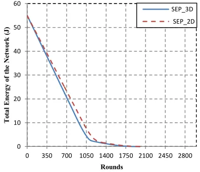
The performance of SEP 3D is compared with that of the original SEP in terms of energy and is shown in Figure 5. With the use of 3D deployment of nodes, the energy consumption of the network is decreased. This is due to the gain of the energy dissipated by height of network. From the graph it is clear that SEP 3D decrease twice the energy savings than SEP protocol.
Figure 5:Energy analysis comparison of SEP 3D and SEP 2D.
The number of nodes alive for each round of data transmission is observed for the SEP 2D and 3D protocols to evaluate the lifetime of the network. Figure 6 and Figure 7 show the performance of SEP 3D compared to SEP 2D. It is observed that the SEP 3D is less perform than SEP 2D due to energy dissipation of individual node throughout the network which depend essentially on the distance between nodes and sink.
0 10 20 30 40 50 60
0 350 700 1050 1400 1750 2100 2450 2800
T
ot
al
E
ner
gy
o
f
th
e
Net
w
ork
(
J)
Rounds
SEP_3D
Figure 6:Number of dead nodes per round comparison of SEP 3D and SEP 2D.
Figure 7:Number of alive nodes per round comparison of SEP 3D and SEP 2D.
Referred to figure 8, it show clearly that SEP 3D provide a poor throughput compared to SEP 2D protocol, this decrease is justified by the low lifetime which give the three dimensional deployment of the nodes in the network.
Figure 8:Throughput SEP 3D and SEP 2D comparison. Generally, we can illustrate the decrease of the SEP 3D in the Figure 9. It’s noted that the throughput decreases about 8% as much than SEP 2D due to its less energy. Whereas, SEP 3D
outperforms the lifetime of SEP 2D by about 10%. In the other hand, SEP 3D consumes about 11% more energy than SEP 2D.
Figure 9:Decrease performances of SEP 3D compared to SEP 2D.
D. Result analysis
From our simulations, we observed that SEP 3D consumes more energy and delivers less packets to the base station. These results can be interpreted by the difference of distance between nodes in both situations which naturally causes by the random deployment of nodes.
E. Optimal value of heterogeneity parameters:
We increase the fraction m of the advanced nodes from 0.1 to 0.2 and a from 1 to 7. Figure 10 and figure 11 show the performance parameters decrease between SEP 2D and SEP 3D. We observe that the best value to approximate 3D-SEP to 2D-SEP is a=4 in the case that m=0.1 and a=5 in the case that m=0.2.
Figure 10: Decrease of SEP 3D compared to SEP 2D for m=0.1.
Figure 11: Decrease of SEP 3D compared to SEP 2D for m=0.2.
0 20 40 60 80 100 120
0 350 700 1050 1400 1750 2100 2450 2800
Nu
m
ber
o
f
dead
n
od
es
Rounds
SEP_3D SEP_2D
0 20 40 60 80 100 120
0 350 700 1050 1400 1750 2100 2450 2800
Nu
m
be
r
of
ali
ve
n
od
es
Rounds
SEP_3D SEP_2D
0 1000 2000 3000 4000 5000 6000 7000
0 350 700 1050 1400 1750 2100 2450 2800
Nu
m
be
r
of
p
ac
ke
ts
t
ran
sm
it
ed
Rounds
SEP_3D SEP_2D
-10.24% -9.93%
-7.81%
-9.93%
-14% -12% -10% -8% -6% -4% -2%
0% FND LND Throughput Energy
De
cr
eas
e
pe
rc
en
tage
(
%)
Performance metrics
-20% -15% -10% -5%
0% 0 1 2 3 4 5 6 7
De
cr
eas
e
(%)
additional energy factor (a)
FND LND Throughput
-15% -12% -9% -6% -3%
0% 0 1 2 3 4 5 6 7 8
De
cr
eas
e
(%)
additional energy factor (a)
VI. CONCLUSION
The analytic of 3D WSN is more complexity than the analytic in 2D WSN. Therefore, many researches approximate 3D WSN space in 2D WSN environment which can provide some error such as the cluster formation. In this paper, we demonstrate by simulation, that this approximation is not reasonable if the height of network is greater than length and breadth of this network.
We strongly believe that projection of WSN in 2D environment is unjustifiable in reason that the 3D WSN is much closer to our physical word.
As future work, we will work to optimize the energy consumption of this network, since the number of cluster head in 3D WSN gives more result than 2D WSN.
REFERENCES
[1] Akyildiz, I. F., Su, W., Sankarasubramaniam, Y., & Cayirci, E. “A survey on sensor networks.” IEEE Communications Magazine, vol. 40, no. 8, pp. 102–114, 2002.
[2] Wang, Y., Shi, P. Z., Li, K., & Chen, Z. K. “An energy efficient medium access control protocol for target tracking based on dynamic convey tree collaboration in wireless sensor networks.” International Journal of Communication Systems, vol. 25, no. 9, pp. 1139– 1159, 2012. [3] C.-T. Cheng, C.K. Tse, F.C. Lau, “A clustering algorithm for wireless
sensor networks based on social insect colonies”, IEEE Sens. J. vol. 11, pp. 711–721, 2011.
[4] A. Thakkar, K. Kotecha, “Cluster head election for energy and delay constraint applications of wireless sensor network”, IEEE Sens. J. vol. 14, no.8, pp. 2658 – 2664, 2014.
[5] W.R. Heinzelman, A. Chandrakasan, H. Balakrishnan, “Energy-efficient communication protocol for wireless microsensor networks”, in: System Sciences, 2000. Proceedings of the 33rd Annual Hawaii International Conference on, IEEE, 2000.
[6] M.S. Ali, T. Dey, R. Biswas, “ALEACH: Advanced LEACH routing protocol for wireless microsensor networks”, in: Electrical and Computer Engineering, 2008. ICECE 2008. International Conference on IEEE, pp. 909–914, 2008.
[7] A. Thakkar, D.K. Kotecha, “CVLEACH: coverage based energy efficient LEACH Algorithm”, Int. J. Comput. Sci. Netw. 1 (2012) [8] M. Handy, M. Haase, D. Timmermann, “Low energy adaptive clustering
hierarchy with deterministic cluster-head selection”, in: 4th International Workshop on Mobile and Wireless Communications Network, IEEE, pp. 368–372, (2002)
[9] G. Smaragdakis, I. Matta, A. Bestavros, “SEP: A Stable Election Protocol for clustered heterogeneous wireless sensor networks”, in: Second International Workshop on Sensor and Actor Network Protocols and Applications (SANPA 2004), (2004)
[10] Wang, Y., Shi, P. Z., Li, K., & Chen, Z. K. “An energy efficient medium access control protocol for target tracking based on dynamic convey tree collaboration in wireless sensor networks”. International Journal of Communication Systems, 25(9), 1139– 1159, (2002)
[11] Ou, S. M., Pan, H., & Li, F. “Heterogeneous wireless access technology and its impact on forming and maintaining friendship through mobile social networks”. International Journal of Communication Systems, 25(10), 1300–1312, (2012)
[12] H.M. Ammari, S.K. Das, “Critical Density for Coverage and Connectivity in Three-Dimensional Wireless Sensor Networks Using Continuum Percolation”. IEEE Trans. Parallel Distrib. Syst. vol. 20, no. 6, 2009.
[13] Baghouri Mostafa, Chakkor Saad and Hajraoui Abderrahmane,“Fuzzy Logic Approach to Improving Stable Election Protocol for Clustered Heterogeneous Wireless Sensor Networks”, International Journal of Computer Science and Network Security (IJCSNS), VOL.14 No.1, January, (2014)
[14] Mostafa Baghouri, Abderrahmane Hajraoui, Saad Chakkor, “Three-Dimensional Application-Specific Protocol Architecture for Wireless Sensor Networks”, TELKOMNIKA Indonesian Journal of Electrical Engineering, vol. 15, no 2, 2015.
[15] Xie, Lijun, and Xi Zhang. “3D clustering-based camera wireless sensor networks for maximizing lifespan with minimum coverage rate constraint”. Global Communications Conference (GLOBECOM), 2013 IEEE. pp. 9-13, 2013.
[16] Attarzadeh, Nima, et al. “Introduce methods for 3D clustering for wireless sensor networks”. Electronics and Information Engineering (ICEIE), 2010 International Conference On. vol. 2, pp. 106-109, 2010. [17] X. Bai, D. Xuan, Z. Yun, T. H. Lai, and W. Jia, “Optimal Deployment
Patterns for Full Coverage and k -Connectivity (k≤6) Wireless Sensor Networks”, IEEE/ACM Transactions on Networking, vol. 8, no. 3, pp. 934 – 947, 2010.
[18] S. Kumar, T. H. Lai, and A. Arora, “Barrier coverage with wireless sensors”, ACM MobiCom, New York, NY, USA, pp 284–298, 2005. [19] C. F. Huang, Y. C.Tseng, and L. C. Lo, “The coverage problem in
three-dimensional wireless sensor networks”, IEEE GLOBECOM, vol. 5, pp 3182–3186, 2004.
[20] M. Watfa and S. Commuri. “A coverage algorithm in 3D wireless sensor networks”. Wireless Pervasive Computing, 2006 1st International Symposium on, IEEE PerCom, 2006.
[21]Linghe Kong, Mingchen Zhao, Xiao-Yang Liu, Jialiang Lu, “Surface Coverage in Sensor Networks”, IEEE Transactions on Parallel and Distributed Systems, vol. 25, no. 1, pp. 234 – 243, 2013.
Baghouri Mostafa was born in Tangier Morocco. He’s a
member in the Physics department, Team Communication Systems, Faculty of sciences, University of Abdelmalek Essaâdi, Tetouan Morocco, his research area is: routing and real time protocols for energy optimization in wireless sensors networks. He obtained a Master's degree in Electrical and Computer Engineering from the Faculty of Science and Technology of Tangier in Morocco in 2002. He graduated enabling teaching computer science for secondary qualifying school in 2004. In 2006, he graduated from DESA in Automatics and information processing at the same faculty. He works as a teacher of computer science in the high school.
Abderrahmane Hajraoui is a professor of the Higher
Education at University of Abdelmalek Essaâdi. He’s a director thesis in the Physics department, Communication and detection Systems laboratory, Faculty of sciences, University of Abdelmalek Essaâdi, Tetouan Morocco. His research areas are: Signal processing and image, automation, automation systems, simulation systems, Antennas and radiation, microwave devices
Chakkor Saad was born in Tangier Morocco. He’s a