Selection an Optimal Control Channel for STATCOM-Based Stabilizers to Damp Inter-Area Oscillation

Selection an Optimal Control Channel for

STATCOM-Based Stabilizers to Damp Inter-Area Oscillation

A. Samanfar

Department of Electrical Engineering, Khoramabad Branch, Islamic Azad

University, Khoramabad, Iran Email: [email protected]

M.R. Shakarami

Department of Electrical & Electronic

Engineering, Engineering Faculty, Lorestan University, Lorestan, Iran

Email: [email protected]

R. Sedaghati

Department of Electrical & Electronic Engineering, Engineering Faculty, Lorestan University, Lorestan, Iran Email: [email protected]

Abstract – In static synchronous compensator (STATCOM) a controllable AC voltage is generated by a voltage-source converter. There are two control channels for controlling of magnitude and phase of the voltage. When these devices are used for damping inter-are oscillations in multi-machine power systems, a damping stabilizer can be applied for both channels. In this paper, a method by quadratic mathematical programming has been presented to design of the damping stabilizer. By this method, the effect of the stabilizer in both control channels of the STATCOM on damping of inter-area oscillations has been assessed. Obtained results on a 2-area 4-machine power system shows that a STATCOM-based stabilizer in the phase control channel is more effective for damping inter-area oscillations than that of the magnitude control channel.

Keywords–Inter-Area Oscillations, STATCOM, Damping Stabilizer, Control.

I. I

NTRODUCTION

Damping of power system oscillations between inter-connected areas is very important for the system secure operation. Conventionally, power system stabilizers (PSSs) are used for damping power system oscillations. However, the use of PSSs may not be only, in some cases, effective in providing sufficient damping for inter-area oscillations, particularly with increasing transmission line loading over a long distance [1]. Nowadays, besides PSSs to damp local modes, power electronics-based FACTS stabilizers have become one of the best alternative means to improve inter-area oscillations damping. SSSC and STATCOM are members of FACTS family that are connected in series and shunt with the system, respectively. The fundamental principle of a SSSC and STATCOM installed in a power system is based on the generation of a controllable ac voltage source by a voltage source converter (VSC) connected to a dc capacitor [2]. There are two control channels to control the magnitude and phase of the voltage, which are the magnitude control channel and the phase control channel. When the SSSC and STATCOM are used for damping of mechanical oscillations, the damping stabilizer can be applied for the both channels. In [3, 4] a SSSC damping stabilizer and in [5, 6] a STATCOM damping stabilizer is used in the magnitude control channel. In [7] a SSSC-based stabilizer and in [8] a STATCOM-based stabilizer is used in the phase control channel. In [9] influence of the SSSC damping stabilizer in the two control channel on damping of inter-area oscillations, has been compared. Results of this research show that SSSC stabilizer in phase control

channel is more effective. But no comparison has been done for STATCOM stabilizer in different control channels to damp inter-area oscillations in multi-machine power systems in the reported literatures.

In this paper, a method based on quadratic mathematical programming is presented to design a damping stabilizer for STATCOM to damp inter-area oscillations. By this method, effects of the damping stabilizer in the two control channels on damping of inter-area oscillations has been analyzed and compared by eigenvalues and nonlinear simulations.

II. P

OWER

S

YSTEM

M

ODEL

A. Generator

In this study, the generators are represented by forth-order d-q axis model. In this case, nonlinear dynamic equations for ithgenerator are [10]:

) 1 (

s i i







  

) 2 (

( )

( ) ( 1)

i i mi d i di qi qi i qi di d i qi

s

M P I E I E

X X I I D







 

   

    



) 3 (

di di di qi FDi qi i

d

E

E

E

X

X

I

T



₀













(





)

) 4 (

qi qi qi i d di i

q E E X X I

T0    (  )

B. Exciter

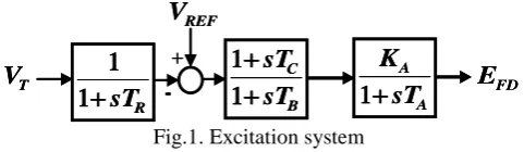
The IEEE type-AC-4A excitation system [11] is considered in this work. Its block diagram is shown in Figure 1.

R

sT



1

1

B C

sT

sT





1

1

A A

sT

K



1

E

FD

T

V

REF

V

+

-R

sT



1

1

B C

sT

sT





1

1

A A

sT

K



1

E

FD

T

V

REF

V

+

-Fig.1. Excitation system

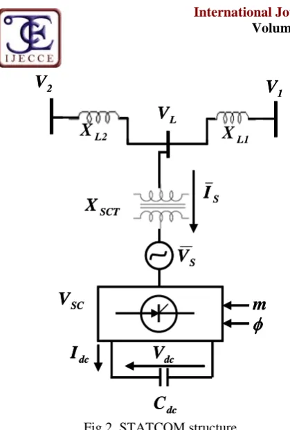
C. STATCOM Modeling

Copyright © 2014 IJECCE, All right reserved 1

V

2

V

2 L

X

1 L

X

SCT

X

S

V

SC

V

_m



dc

I

V

_dc

dc

C

S

I

L

V

1

V

2

V

2 L

X

1 L

X

SCT

X

S

V

SC

V

_m



dc

I

V

_dc

dc

C

S

I

L

V

Fig.2. STATCOM structure

The STATCOM consist of a series coupling transformer (SCT) with the leakage reactance XSCT,a three-phase GTO

based voltage source converter (VSC) and a DC capacitor. These devices can be described as [3, 5]:

) 5 (

j

mkV

V

_S



_dc

(cos





sin



)

) 6 (

I

jI

I

I

_S



_SD



_SQ



_S





) 7 ( ) sin I cos I ( C mk dt dV SQ SD dc

dc_ _ 

where Vsis the generated AC voltage by voltage-source

inverter; m and  are the modulation ratio and phase defined by pulse width modulation (PWM), respectively; k is the ratio between the ac and dc voltage depending on the converter structure; Vdcis the dc voltage; Cdc is the dc

capacitor value, and ISDand ISQare D-and Q components

of the current IS, respectively.

III. STATCOM-B

ASED

S

TABILIZERS

A phase based stabilizer for STATCOM is shown in Fig. 3. In this case, the stabilizer is called the phase-based stabilizer and for convenience in this paper, it is called -based stabilizer. In this stabilizer, TW is washout time

constant; T is stabilizer time constant, and x2, x1and x0are

parameters to be determined. The feedback signal for the stabilizer is selected among local signals as the line-current, the line-real power, and the line-reactive power. To control the magnitude of the injected voltage, modulation ratio m can be controlled. Fig. 4 shows the block diagram of the controller in this case.

Damping Stabilizer W W sT sT sT x s x s x     1 ) 1 ( 2 0 1 2 2 s K K I P S sT  1 1  ref  dcref V dc V -+ + Input Signal Vdc U max Vdc U min + + Damping Stabilizer W W sT sT sT x s x s x     1 ) 1 ( 2 0 1 2 2 s K K I P S sT  1 1  ref  dcref V dc V -+ + Input Signal Vdc U max Vdc U min + +

Fig.3. Phase controller for STATCOM with a damping stabilizer Damping Stabilizer W W sT sT sT x s x s x     1 ) 1 ( 2 0 1 2 2 s K K I P S sT  1 1 ref m Lref V L V -+ + Input Signal Vac U max Vac U min + + m 1 0 Damping Stabilizer W W sT sT sT x s x s x     1 ) 1 ( 2 0 1 2 2 s K K I P S sT  1 1 ref m Lref V L V -+ + Input Signal Vac U max Vac U min + + m 1 0

Fig.4. STATCOM magnitude controller with a damping stabilizer

IV. S

TABILIZER

D

ESIGN

The method adopted in this work to design a STATCOM stabilizer is an incremental method. This method is summarized as follows. In the first step, the closed- loop system is considered as in Figure 5, where G(s) and F(s) are the power system transfer matrix and the stabilizer transfer matrix, respectively. In the second step the stabilizer transfer matrix is changed by F. In this case,

the closed-loop system changes as shown in Figure 6, where G(s) is the transfer matrix of the inner loop between G(s) andF(s). In these Figures, Uref is

considered as the input signal of the system. In the phase-based stabilizer Uref is replaced with Vdcref and in

magnitude based stabilizer it is replaced with mrefand VLref

for STATCOM, respectively. One of the local signals is selected as the feedback signal for stabilizer. The value of

F is calculated to shift eigenvalues of critical modes to

desired values.

)

s

(

G

)

s

(

F

Local

Signal

+

+

ref

U

_G

₍

_s

₎

)

s

(

F

Local

Signal

+

+

ref

U

)

s

(

G

)

s

(

F



Local

Signal

+

+

ref

U

_G

₍

_s

₎

)

s

(

F



Local

Signal

+

+

ref

U

Fig.6. Closed-loop system in the second step In the following, a procedure for calculation of F is

presented. Assuming variations ofF is sufficiently small, the variation of the eigenvalueican be approximated as

) 8 (

f _i

i i  ()

  

 (i=1, 2, ..., n)

where n is the number of critical eigenvalues andiis the

residue associated to the ith eigenvalue i of

G

(

s

)

.

Equation 8 can be rewritten as

) 9 (

 



 



 



 







 



 



 



 





i i i i



i i

i i

i

f f

j

f f

 

 

 

 



 

 

 

 



Re Im Im

Re

Im Im Re

Re

It is assumed that the stabilizer has a lead-lag structure as follows:

) 10 (

w w

sT sT sT

x s x s x s f

 

  

1 ) 1 ( ) (

2 0 1 2 2

By substituting

s





_i and

x

_m





x

_m(m=1, 2, 3) in Equation 10, the real and imaginary part variations off

(i) are

) 11 (

0 0 1 1 2

2 x R x R x

R ) ( f

Re(





_i  _i



 _i



 _i



) 12 (

0 0 1 1 2 2

)

(

Im(



f



_i



I

_i



x



I

_i



x



I

_i



x

where R0i, R1i, R2i, I0i, I1i, and I2iare specified values. To

shift critical eigenvalues to the left of the imaginary axis, we must have

) 13 (

i i  

 )

Re(

) 14 (

i i

i













 

 Im( )

where i and iare the desired shift value of the real

part and acceptable frequency variations of the critical eigenvaluei, respectively. Substituting Equations 11 and

12 in Equation 9, we can obtainias the linear function

fromx2,x1and x0. Then, substituting the real part of

iin Equation 13 and its imaginary part in Equation 14

yields

) 15 (

i i

i

i



x





x





x







_{2 2}



_{1 1}



_{0 0}





) 16 (

i i

i i

i





x





x





x









   

 2 2 1 1 0 0

where0i,1i,2i,0i,1i, and2iare specified values. On

the other hands, if the angle of residue iis positive, the

stabilizer must have a phase-lead characteristic; otherwise, it must have a phase-lag characteristic. Assuming

sT

s



and substituting in Equation (10) yields

) 17 (

s

T

T

s

T

s

s

x

s

x

x

s

f

w w











1₂

2 2

)

1

(

1

0

)

(





where

x

ˆ

₂and

x

ˆ

₁are defined as

) 18 (

2 0

2 2

T

x

x

x





) 19 (

T

x

x

x

0 1

1





Function

f

(s

)

has a double pole at

s



-1. According to ref. [12] For a phase-lead structure, it is assumed that zeroes of

f

(s

)

are almost one-decade nearer to the center than that of its poles, i.e., they belong to interval [-1 -0.1] and for the phase-lag structure the zeroes are almost one decade further to the center, i.e., they belong to interval [-10 -1]. This subject is graphically shown for lead and lag structure in Figures 7 and 8, respectively.

In this figures the points inside the triangles and above the parabolas correspond to above intervals. To represent the constraints as linear function, the parabolas are approximated by lines. In this case the zeros may be as complex values, but real part of the complex zeros are located in above intervals.

Fig.7. Region corresponding to phase- lead stabilizer

Fig.8. Region corresponding to phase- lag stabilizer According to Figure 7, the constraints for phase lead structure can be written as

) 20 (

Copyright © 2014 IJECCE, All right reserved

) 21 (

10 x 1 . 0 x₁ ₂

) 22 (

180 x 18 x

99 1 2 

As illustrated in Figure 8, the constraints for phase lag stabilizer are

) 23 (

1 x x₁₂

) 24 (

1 x 100 x

10₁ ₂ 

) 25 (

18 x 180 x

99 ₁ ₂ 

  

Substituting Equations 18 and 19 in Equations 20 to 25 and assuming

x

_m





x

_m



x

_m(m=1, 2, 3) where

x

₀,

1

x

and

x

₂ are known values, the constraints can be rewritten for lead structure as Equations 26 to 28 and for lag structure as Equations 29 to 31.

) 26 (

0 2 1 2 0 2 1

2 T x T x x Tx T x

x     









) 27 (

2

2 1 0

2

2 1 0

10 100

10 100

x T x T x

x T x T x

     

 

) 28 (

2

2 1 0

2

2 1 0

18 99 180

18 99 180

x T x T x

x Tx T x

     

  

) 29 (

0 2 1 2 0 2 1

2 T x T x x Tx T x

x     

  

) 30 (

2

2 1 0

2

2 1 0

100 10 100 10

x T x T x

x Tx T x

      

  

) 31 (

2

2 1 0

2

2 1 0

180 99 18

180 99 18

x T x T x

x T x T x

     

  

The following function, as the gain of the stabilizer at the frequency



_i, i=1, 2, . . . m, is considered as the objective function[13].

) 32 (

 

2

m

1 i

i

j f min

J









where



₁,



₂...,



_m are a set of frequencies in the region where the critical eigenvalue must be shifted. By substituting Equation 10 in Equation 32 and considering

s



j



_i and

X



X





X

, we can easily rewrite the objective function as

) 33 (

1 min

2

T T

J  X H X f X

where the matrix H, vector f and vector

X





x₂ x₁ x₀



Tare known and

X

 T

x x

x ]

[ 2  1  0

 is the unknown vector to be tuned. Equation 33 with Equations 15 to 16 and Equations 26 to 28 or Equations 29 to 31 is as a quadratic mathematical programming problem. To solve this problem the

quadprog algorithm provided by the Matlab Optimization

Toolbox is applied here. The proposed approach is an iterative method. In this method calculated vector ofX is

added to the known vector

X

and it is considered as known vector in the next iteration. The vector

X

in the first iteration is set to be zero.

V. S

IMULATION

R

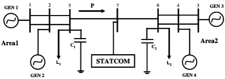
ESULTS

The case study here is a 2-area 4-machine power system. A single line diagram of the system is shown in Figure 9. Data of this system is represented in [14]. To control inter-area oscillations, a STATCOM is installed at bus 7. Specific parameters used for the STATCOM are given in the Appendix. The loads are modeled as constant impedances.

L1

C1

L2

C2

GEN 4 GEN 3

GEN 2 GEN 1

Area1 Area2

STATCOM P

1 2 5 7 6 4 3

L1

C1

L2

C2

GEN 4 GEN 3

GEN 2 GEN 1

Area1 Area2

STATCOM P

1 2 5 7 6 4 3

Fig.9. one-line diagram of the 4-machine power system In this system, three operating scenarios based on the transmitted power between the interconnected areas are investigated. To increase transferred power, the load in area 2 has been increased and the load in area 1 has then been modified to achieve a given tie-line transferred power. The summary of operating conditions that are studied in this paper is shown in Table 1.

Table 1: The summary of operating conditions Load Area

2 (MW) Load Area

1 (MW) Power

transfer (MW) Loading

Conditions

1180 1120

180 Light

1380 920

380 Normal

1410 890

410 Heavy

Inter-area mode at different operation conditions for the system installed with a STATCOM without damping stabilizer (open- loop) are shown in Table 2. It is clear that damping ratio of inter-area mode is reduced by increasing transmitted power and it close to instability in heavy loading conditions.

Table 2: Inter area mode and its damping ratio in open-loop system

Loading

Conditions Inter-area mode

Damping ratio

Light -0.348±j3.003 0.1151

Normal -0.326±j3.318 0.0978

Heavy -0.241±j2.967 0.0809

According to the designed method, a signal with the maximum residue for the inter-area mode is selected as the feedback signal for the damping stabilizer. Table 3 shows residues for the inter-area mode for different operating conditions. It can be seen from this table that:

 Variation of the current in the transmission line is the best signal forand m -based stabilizer.

Table 3: Residues for inter-area mode for different signal in the 4- machine power system

Parameters of stabilizers are typically calculated at heavy loading conditions. It is assumed that the desired damping ratio for the inter-area mode is = 0.25. According to the frequency of inter-area mode in the open-loop system, the value of



_iin Equation 32 has been considered _i =1, 3, 5. The time constant of stabilizer is set as T=0.4. Also, the effects of stabilizer on other modes particularly local modes must be considered so that the damping ratio of other modes has been increased or does not become less than a specific value and the variations of their frequencies must be acceptable. To improve the damping ratio of inter-are mode to a desired value, the parameters of the proposed STATCOM-based stabilizers are calculated and shown in Tables 4 at heavy loading. In this table the loop gains of stabilizers in the frequency close to inter-area mode (f (j)) are shown. Typically, loop gains are calculated at = 3.5. This value show that to achieve the same damping ratio, the gains of the  -based stabilizer are less than the gains of the m -based

stabilizer. In other words, the  -based stabilizer is more effective for the damping of inter-area oscillations.

Oscillation modes in open and close-loop system are shown in Table 5. This table shows that damping ratio of the inter-area mode has been improved to the desired value. In addition, it can be seen that other modes have not been degraded significantly.

Table 4: Parameters of the proposed STATCOM-based stabilizer at heavy loading

Stabilizer x2 x1 x0 f(j)

m -based 0.5008 0.6760 0.1376 2.177

-based 0.0948 0.2651 0.1947 0.452

Table 5: Oscillation modes in the system installed with STATCOM at heavy loading

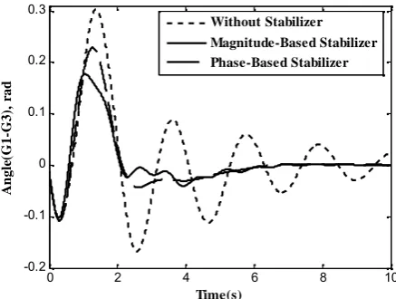
For completeness and verification of the designed stabilizers, a three-phase fault was applied to the test system at bus 6. The fault is cleared without line switching. Because generators 1 and 3 have the most contribution in the inter-area mode, typically, the swing angle of generator 1 with respect to generator 3, in the both control channels, for STATCOM stabilizers are shown in Figures 10. This figure shows that STATCOM stabilizers can effectively damp inter-area oscillations. Control signals of STATCOM damping stabilizers are shown in Figures 11. It can be seen that the  -based stabilizer provides much less control effort compared to that of the m -based stabilizer.

0 2 4 6 8 10

-0.2 -0.1 0 0.1 0.2 0.3

Time(s)

A

n

g

le

(G

1

-G

3

),

r

a

d

Without Stabilizer Magnitude-Based Stabilizer Phase-Based Stabilizer

Fig.10. Swing angle of G1 relative to G3 in the system installed with STATCOM for fault duration of 0.05s

0 2 4 6 8 10

-0.4 -0.3 -0.2 -0.1 0 0.1 0.2 0.3

Time(s)

C

o

n

tr

o

l

S

ig

n

a

ls

(p

u

)

Magnitude-Based Stabilizer Phase-Based Stabilizer

Figure 11. Control signals of STATCOM stabilizers with fault duration of 0.05s

VI. C

ONCLUSION

Copyright © 2014 IJECCE, All right reserved result by eigenvalue analysis and nonlinear simulations on

a 2-area 4-machine power system show that a STATCOM stabilizer in phase control channel, comparing the magnitude control channel, is more effective for damping of inter-area oscillations.

A

PPENDIX

Parameters used for STATCOM (in p.u., unless specified) are presented in Table A1.

Table A1: Known parameters for STATCOM TS XSCT Cdc Vdcref

DC Voltage Regulator

AC Voltage Regulator

KP KI KP KI

0.01s 0.15 1 1 1 50 1 1

R

EFERENCES

[1] M. Noroozian, M. Ghandhari, G. Anderson, J. Gronquist, and I. A. Hiskens. “A robust control strategy for shunt and series reactive compensators to damp electromechanical oscillations”,

IEEE Trans. Power Del., vol.16, no. 4, pp. 812-817, 2001.

[2] I. papic, “mathematical analysis of FACTS devices based on a voltage source converter Part 1: mathematical models”, Elect. Power Syst. Res., vol. 56, pp. 139-148, 2000.

[3] H. F. Wang, “Static synchronous series compensator to damp power system oscillation”,Elect. Power Syst. Res., vol. 54, no. 8,

pp. 113-119, 1999.

[4] A. Kazemi, M. Ladjevardi, and M. A. S. Masoum, “Optimal selection of SSSC Based damping stabilizer parameters for improving power system dynamic stability using genetic algorithm”, Iranian Journal of Science & Technology, Transaction B, Engineering, vol. 29, no. B1, pp. 1-10, 2005.

[5] H. F. Wang, “Pillips-Heeffron model of a power system installed with STATCOM and application”, IEE Proc.-Gener. Transm. Distrib., vol.146, no. 5, pp. 521-527, 1999.

[6] D. Z. Fang, “Coordinated parameter design of STATCOM stabilizer and PSS using MSSA algorithm”,IET Gener. Transm. Distrib., vol. 1, no. 4, pp.670-678, 2007.

[7] F.A.L. Jowder, “Influence of mode of operation of the SSSC on the small disturbance and transient stability of a radial power system”,IEEE Trans. PWRS, vol. 20, no. 2, pp. 935-942, 2005.

[8] M. A. Abido, “Design of PSS and STATCOM-based damping stabilizers using genetic algorithms”, in Proceedings of the IEEE General Meeting on Power Engineering Society, Canada,

Montreal, pp. 1-8, 2006.

[9] M. R. Shakarami, and A. Kazemi, A, “Assessment of effect of SSSC stabilizer in different control channels on damping inter-area oscillations”, Energy Conversion and Management, vol. 52, pp.1622-1629, 2010.

[10] Sauer, P. and Pai, M., Power system dynamics and stability, Prentice Hall, New Jersey (1998).

[11] P. M. Anderson, and A. A. Fouad, Power system Control and

stability, Iowa, Iowa State Univ. Press (1977).

[12] R. C. Dorf, and R. H. Bishop, Modern control systems, Prentice Hall (2005).

[13] L. C. Zanettaand, and J. J. Da Cruz, “An incremental approach to the coordinated tuning of power system stabilizers using mathematical programming”,IEEE Trans. PWRS, vol. 20, no.1,

pp. 895-902, 2005.

[14] S.Liu, A. R. Messina, and V. Vittal, “Assessing placement of controller and nonlinear behavior using normal form analysis,”