An analysis of methods and
approaches to evaluating reliability
when predicting equipment failures
by Oleg V. Aralov and Ivan V. Buyanov*
Pipeline Transport Institute, LLC, Moscow, Russian Federation
T
HE QUALITY OF EQUIPMENT plays an important role in ensuring its reliability. The production of poor-quality goods at manufacturing facilities can be avoided when the manufacturer observes the requirements of state standards, construction regulations and rules, technical specifications. etc. However, checking that the manufacturer is complying with these requirements is rather complicated.The authors of this article have analysed approaches to creating a mathematical tool capable of making a quantitative and qualitative prediction of equipment failures, evaluating current operational readiness, and determining the optimum degree of load to ensure principles of maximum reliability and conservability.
Approaches to quantitative predicting equipment failures, developed and described using the research results, could be introduced into the current system of conformity assessment, given that there is a sufficient amount of statistical data regarding equipment functioning. These data have been collected by Transneft PJSC, over the last decade.
Keywords: conformity assessment, reliability, product quality, equipment failure prediction, mathematical tool, oil pump
Corresponding author’s contavt details: e-mail: buyanovib@niitnn.
transneft.ru
Introduction
The system of trunk pipeline transportation for hydrocarbons includes a large quantity of equipment designed for various technological operations. The variety and number of types of equipment depends on the types of production facilities at which it is used. For example, various shut-off, control, and safety valves, pipeline systems, cathodic, ground, and drainage protection systems etc. are used at linear facilities. Crude oil quality control systems (CQCS), tank farms with service equipment, mechanical and power equipment for pumping hydrocarbons (main-line pumps and electric motors) are used at site facilities. In this article, an oil-pumping units (OPUs) will be examined
as an integrated facility consisting of a multitude of structural modules.
models: today, around 20 basic models of main-line pumps are in use. This increases the variety of assemblies of different versions (up to approximately 500 options).
Considering the variety of OPU options, a general diagram is presented here in simplified form for ease of analysis (Fig.1).
An OPU as a multi-component equipment has a large number of failure types, which can be divided into two basic groups: latent factory, and operational. As a result of analysis, it has been established that in the period from 2013 to 2015, 64% of irreparable OPU failures affected main-line pumps, and only 36% affected electric motors. This indicates that main-line pumps are by far the least reliable element of OPU. The division of the specific quantity of failures into the separate types most characteristic for OPU is shown in Fig.2.
In accordance with the database for the products quality assessment (QA DB), which is being developed by the leading scientific research institute at Transneft PJSC, all types of OPU failures were sorted into specific groups for the period from 2013 to 2015. The groups were based on similarities in the reasons why the failures occurred. The basic types of OPU failure are shown in Fig.3, where the blue boxes mark types of failures related to the electric drives, and the black boxes mark those related to the main-line pumps. As
can be seen, the reasons for these failures may have either factory or operational character.
The specific number of operational failures out of the total number of failures at main-line pumps was determined through detailed analysis, which involved identification of the basic reasons for the failures to occur. They include:
• imperfections in the construction of the frame at the manufacturing plant;
• the presence of defects in the main line pump case castings;
• insufficient reliability of attachment fixtures for the bearings and pump shafts;
• axial shift of the pump shafts;
• poor quality repair and maintenance works;
• rapid changes to the operating parameters of main-line pumps.
During analysis it was established that the specific number of operational failures was 47%, while the remaining 53% belonged to the category of latent factory failures.
A conformity assessment system has been created at Transneft PJSC aimed at preventing the appearance of failures and worsening equipment characteristics during operation. This assessment is carried out in order to establish the conformity of manufactured articles to
Motor Pump
Explosion-proof synchronous electric motors; •General-purpose industrial synchronous electric motors; •Electric motors with voltage of 6(10) kV, for main line and booster OPUs; •Horizontal explosion-proof
induction electric motors; •Vertical explosion-proof induction electric motors;
Oil and oil-product centrifugal main line pumps and electric pump units on their basis
the technical regulations of EurAsEC (the EU Customs Union and the Russian Federation), to national standards, construction rules and regulations, the high-level budget estimates, as well as to general and special technical specifications (GTS and STS respectively), where they do not contradict federal regulations. GTS and STS are developed on the basis of integrated scientific studies and set the requirements for the most significant types of equipment and materials with the aim of ensuring the greatest safety of hydrocarbon transportation.
Given the imperfect nature of equipment and technological process, an accumulation of latent fatigue stresses can be observed fairly often at various stages of product manufacture. These stresses are impossible to detect during the outgoing inspection, carried out by the manufacturer, of the given product type when it is released to the customer.
In turn, it is also difficult to assess the presence of latent factory defects during the incoming inspection when the equipment is delivered.
Latent defects become apparent after the acquired product has run many operating cycles. This significantly complicates assessing the nature of the occurrence of the given defect at its non-steady state. Given these conditions, it seems hard to prove the natural or accidental reason of the defect’s occurrence without statistical processing of a large sample group of defects in this type of products, which have the same sorts of failures during operation.
Where a defect which has arisen during operation of some type of product is naturally-occurring (i.e. is occurs due to the development of a latent defect), then there are grounds for increasing the requirements for the equipment Fig.2. Specific quantity of the most characteristic failures for OPU, %:
in use and toughening the system for assessing it. It should be noted here that the development of company in-house requirements for product quality is grounded in the necessity of ensuring maximum safety and the operating conditions specific to that company. The quality requirements for manufacturing the basic product types in operation at Transneft PJSC have a scientific basis in the R&D results for creating various methods to establish the reasons for defects arising, identifying optimal operating modes for equipment, etc.
Methodology
The delivery of high-quality equipment by manufacturers guarantees its reliability during operation. However, in practice cases of manufactured defective goods can be found. Moreover, manufactured defective goods may include both obvious defects and latent defects, which may lead to failure in certain operational conditions. Manufactured defective goods can also be understood as products
released with sufficient deviation (both in design features, and materials used) from the actual operating conditions that, in the future, will also lead to the incidence of failure. The occurrence of poor-quality (defective) products at manufacturing facilities can be avoided if the manufacturer complies with the requirements of state standards, construction rules and regulations, technical specifications, etc. However, it is extremely challenging to check whether a manufacturer is complying with these requirements. The solution can be found in the organization of multi-level procedures for incoming goods inspections from manufacturers, which should be based on the internal requirements of the customer. This method has been implemented effectively by Transneft PJSC where a register of basic types of goods is being formed and updated.
A current priority is creating a separate methodological tool, which would allow qualitative and quantitative predictions of failures to be made, and the equipment’s current operational readiness to be Motor
Electrical
Pump
Mechanical
1. Defect in the insulation of the electric motor case; 2. Defect in the insulation on the stator winding; 3. Failure of the vacuum circuit-breaker; 4. Short-circuit in the rotor winding; 5. Failure of the protective thermal resistor; 6. Loose anchoring for foundation;
7. Emergency temperatures of the stator winding.
1. Defects in the welded joints; 2. Defects in the impeller casting; 3 Insufficient frame stiffness; 4. Defects in the seal membranes; 5. Defects in the pump case casting;
6. Other mechanical defects in the form of through-thickness cracks, pores etc.;
7. Damage to the bearings; 8. Axial shift of the shaft; 9. Leakage of mechanical seals;
10 Increased vibration and noise of the bearing units;
11. Rotor disbalance;
12. Emergency temperatures of the stator winding.
assessed. It would also enable the optimum utilization rate to be identified, in order to ensure maximum reliability and conservability (here the equipment characteristic is implied, which is described by the indicator ‘average period of conservability’).
At present there are methods in Russian and international practice which allow the technical condition of equipment during operation to be determined, and prediction of its behaviour after a certain number of operating cycles. However, none of the methods analysed in this article allows for a solution to identifying the original reason for a defect to arise, which casts doubt on their practical use. It is therefore a relevant and promising direction of research to develop a methodological tool which would allow companies in the oil and gas industry to make qualitative and quantitative predictions of equipment failure.
As a result of this analysis, it has been established that the following methods are the most relevant in terms of applied mathematical approaches and possibilities of evaluating the system’s technical condition:
• integrated condition monitoring of the dynamic objects and systems;
• point estimation of the probability of failure-free work in a technical system, based on a complete sample group (‘failure-free’ is understood as the equipment characteristic, which is illustrated by such indicators as the probability of failure-free operation, the mean time between failures (MTBF), the mean time to failure (MTTF), the failure rate);
• calculating the probability of detecting defects, initial and residual defectiveness using results from non-destructive inspection; • constructing probability models
of reliability based on sample groups of current conditions;
• computational-experimental method of evaluating reliability
indicators for the system as a whole, based on results of separate tests for the reliability of its components.
It should be noted that the method of point estimation of the probability of failure-free work in a technical system, based on a complete sample group, involves computational technology. It may be used when analysing and making an exact estimation of the information for reliability indicators for a technical system. It enables to develop a tool capable of automating the point estimation of the probability of failure-free work in a technical system based on a complete sample group. The functional of the tool is attained by using a specific number of computational blocks with specially organized links between them, which enable to implement the method of point estimation of the probability of failure-free work in a technical system, based on a complete sample group. This method can be expressed mathematically with the formula:
P t p P t t p d t t N
N N
∧
= + − −
* ( ) 0( ) ' (1 ) 1 ( )'' ''
where:
t = the length of operating time, in hours
ˆ *( )
P t is the probability of a work failure arising during the operating time
P0(t) = is the a priori value of the probability of failure-free work during the operating time
d(t) = the number of failures observed in the interval of time between 0 and t
N = the number of experiments for which the operating time of the technical system was calculated pN = the relativity factor, which
characterises the share of a priori information impact on the probability estimation for failure-free work, calculated according to the formula:
p N
N =
where:
β is the number of events which involved receiving reliable information about the probability estimation for failure-free work.
The method described here allows a point estimation to be made for the probability of failure-free work in the system, i.e. to assess its discrete value. In practice, however, a continuous estimate of the system’s technical condition is needed. This can lead to the distortion of received results and severely delayed responses in the system when applying this method to the non-discrete inspection types.
The method of calculating the probability of detecting defects, initial and residual defectiveness using the results of non-destructive inspection is distinguished by the fact that for a specific product or group m of the products of same type, the critical dimensions
c
cs of the defects in operational mode can be calculated, together with the dimensions [c
]po. of defects which are permissible in operation, and the dimensions [c
]pmof defects which are permissible in manufacturing. The results of the inspection are presented in the form of a bar graph in coordinates (Ndd, c), where Nddis the number of defects found during the inspection, and c is the typical size of a defect. The required bar graph can be approximated with the equation:N
A exp
dd n
χ
χ η α χ χ η
( )
=– – – – –
{ ( ) [ ( )] }
– 1 1
0
N
A exp n exp
dd χ
χ η χ χ η
( )
=– – – – – –
( ) { 1 (1 ) [ (1 0)] }
where:
A, n, α, η are constants which are calculated based on approximating as much as possible the Equn Ndd(c) to the results of the inspection, presented in the form of a bar graph;
c 0 is the minimum defect size which may be detected.
The initial defectiveness Nres can be calculated using the formula:
Nid A n or N A exp n id
, –
–
= χ =
(
χ)
The probability of detecting a defect Ppdd is calculated using the formula:
Ppdd=1 1– –
(
η)
exp[ (–α χ χ– 0)]–ηIn turn, the residual defectiveness Nres is calculated as the difference between Ndd and Nres.
The method of calculating the probability of detecting defects, both initial and residual, using the results of non-destructive inspection largely depends on the input parameters of the inspection, and specifically on the values of permissible and critical defect sizes during operation and manufacture. It is practically impossible to acquire this information for all types of defect from companies in the oil and gas industry due to the large quantity of the latter. Moreover, the estimation of defect sizes in equipment which is necessary for calculations significantly complicates the process of this probabilistic method implementation.
results of assessing the condition of the dynamic system.
The method examined here allows the condition of the technical system during operation to be determined fairly accurately, but at the same time it entirely fails to fulfil the requirement for finding a reason for failure to occur. Therefore, using the mathematical process described for this method of assessing the condition of dynamic objects and systems may be effective for solving the task formulated here, but under the condition of reorganizing the process of statistical and probabilistic evaluation. Theoretically, this reorganization can be carried out by combining the method of integrated condition monitoring of the dynamic objects with the methods described above: the method of point estimation of the probability of failure-free work in a technical system based on a complete sample group, and the method of calculating the probability of detecting defects, initial and residual defectiveness using the results of non-destructive inspection (both taken separately and in combination).
The combination of the methods listed above allows the moment when a defect is formed to be identified, as well as the degree of its development, and the probability of a similar defect occurrence, as well as the reason of it occurrence can be approximately determined. However, it is still very difficult to identify precisely whether the defect’s appearance has a natural or accident-related nature. Taking into account the fact that the initial parameters characterizing the defect during analysis should not be used when forming a methodology for evaluating the product’s technical condition due to increase of mathematical error in the model obtained, it may be concluded that using a combined approach to establish the technical condition of the equipment is not advisable.
In contrast to the methods of determining the technical condition of equipment outlined above, a method of forming a probability model for reliability based on
sample groups of the current conditions, and a computational-experimental method of evaluating indicators for the reliability of the technological complex based on the results of separate tests of the reliability of its components, seems to be more independent and universal for their approbation in real equipment operating conditions at oil and gas industry enterprises.
The method of building probability models of reliability based on samples groups of current conditions involves designing the probability model of failures based on the results of equipment reliability tests. In the case of the accident-free operation, there exists the observation ordered from the right; while if the device failed, it means that the failure occurred before the moment of testing, and the observation is ordered from the left. The obtained sample group of the observations ordered from the left and from the right (without full observations) is called the sample group of current states, after which it becomes possible to calculate the relationship of the Fisher information quantity regarding parameters in the sample group of current states to the Fisher information in the full sample group. As a result of maximizing the Fisher information quantity, the optimal moments for testing the products can be established (from the standpoint of highest likelihood evaluation accuracy).
This method allows the duration of testing products to be fully evaluated in order to detect the maximum quantity of embryonic defects in the equipment. However, its use to determine the technical condition of the equipment without excluding the latter from technological processes does not seem to be possible.
parameters, which allow the equipment’s current condition to be determined using the values of reliability indicators. As the method described previously, this method is not appropriate for most of equipment at oil and gas industry enterprises (this is especially true for process equipment units, which do not have technical back-up), because it is impossible to carry out
inspections without excluding equipment from the technological process.
Evidently, there is an insufficient quantity - both in Russian and international practice - of methods which enable equipment failure to be predicted using statistical probability (and which satisfy the relevant technical specifications). It can thus be
Oper
ating time of the eq
uipment, months
Failure rate, 1/month
Average at Transneft PJSC
An individual unit of equipment
Fig.4. A comparison of the equipment failure rates versus operating time for pumps from an arbitrary series between the following values:
Failur
e int
ensity
, 1/time; number of f
ailur
es
Operating time
concluded that creating a mathematical process which is capable of making a quantitate and qualitative prediction of equipment failure, evaluating its current operational readiness, and determining the optimum capacity utilization rate to ensure the principles of maximum reliability and conservability, is a topical and promising area for R&D studies.
Results
The proposed mathematical model will be based on the Weibull distribution, the key variables of which will be failure rate and the equipment operating time. The failure rate is the apparent density of equipment failures, calculated for the moment in time under examination or for the operating time, given the condition that before this moment no failure had occurred. It is worth noting here that the Weibull distribution used in this case may have a much more informative character. The established values of average failure rates for separate types of equipment may also be used to make a quantitative prediction of failures, in particular the quantity of failures in separate batches of a given type of equipment.
Correlations are outlined below which enable the number of equipment failures to be predicted based on specific intervals of operating time with reference to the average values for equipment failure rate, calculated for all units of technological equipment in operation at Transneft PJSC.
The basis for the proposed functions is the assumption that all similar modifications and types of equipment have analogous quantitate and qualitative characteristics regarding failures. In other words, if on average at Transneft PJSC pumps from an arbitrary series (for example single-section pumps of the NM series) have the curve of failure rate versus operating time, shown in Fig.4 by the blue curve, then individual pumps of the same series will have analogous characteristics for failure rate versus operating time, as shown by the red curve.
This assumption means that when using the characteristic for failures of all units of individual process equipment in operation at Transneft, PJSC over a specific interval of time, values can be calculated for certain intervals of the operating time. These values will be fair both for individual units of equipment of the given type in the time range under examination, and for equipment issued or brought into operation during a period not corresponding to the original time interval.
Assigning the task of predicting the number of equipment failures at certain stages of the operating time can be formulated in the following way. This assumes known average values of failure intensity at the necessary stages, determined for equipment of this type on average at Transneft PJSC.
Assume that for a certain type of equipment, the relationship between failure intensity and the total operating time has been established (Fig.5). Then the individual units of the equipment of this type, as was mentioned above, will have analogous characteristics. That is, at separate time intervals the number of failures may not coincide with the average arbitrary value, calculated for the whole codification series; however, the function will be in a form comparable to the general function.
Supposing that for a certain modification of an arbitrary type of equipment, statistics were collected regarding failures over a set period of time. Figure 5 shows the failure rate for a given equipment versus the operating time (blue curve), as well as the change in the specific number of failures which occurred at a certain interval of time versus the total operating life of the equipment (green curve). If these curves are divided at certain time intervals, then each interval will be characterized by its own value for failure rate for equipment λ and by the number of equipment failures r. That is, the time interval examined Dti will have its own corresponding values λi and ri.
relationship of the failure rate, calculated for all units of equipment of a specific type, will be the basic function, i.e. the values for failure rate, established for individual units of technological equipment, will tend towards the given function by their absolute value. Thus, for the interval ∆ti:λi1 →λiwhere λi1is
the failure rate, calculated for an individual unit of the process equipment.
This assertion can be confirmed by the fact that the equation for failure rate alters in proportion to the ratio r t
Nav
∆
( )
.This is because it is functionally dependent on only two dynamic parameters: the number of failures in the specific interval of operating time and the average quantity of equipment properly functioning in a specific interval of operating time. This also accounts for the fact that in order to describe the failure rate curve for equipment of a certain type as a whole at Transneft PJSC, the proportional relationship r t
N
i i
( )∆
∑
∑
avis
used, which is an additive ratio of the separate elements r t
Nav
∆
( )
.These elements characterise the functional interrelation of the failure quantity for equipment for a certain interval of operating time and the average quantity of operational equipment at a given time interval. That is, coefficients obtained for the given correlations will co-ordinate: at corresponding stages it is highly likely that the dynamics of change in the failure quantity (either on the positive or the negative side) in comparison with the former stage will be identical. This serves as the basis for the possible use of failure rate values for a certain type of equipment established at Transneft PJSC for predicting the number of failures for
separate units of process equipment in the future.
Number of failures for one unit (several units, or batch) of equipment should be calculated at stages of its lifetime cycle. For this common failure rate values for equipment at separate time intervals are established, as well as the initial value for the number of failed equipment. For example, for the time interval r(Dt)i–1 (denoted by the solid blue and solid black curves in Fig.5) a curve is shown for equipment failures, which should be obtained. The crosshatched area in Fig.5 depicts the first interval of time at which it is necessary to predict the number of equipment failures, the interval of time is marked out (by the green area) which is characterized by a specific number of equipment failures (as initial data for calculation).
Having denoted the target value for the number of equipment failures in the predictable time interval r(Dt)’, this value can be expressed through the general equation for failure rate:
r t N t
r t N t N t r t t
av
∆ ∆
∆ ∆ ∆
( )
== + −
'
( )' { ( ) [ ( ) ( )']} , λ
λ 0 0
2
(1)
where N0(t) is the quantity of properly functioning equipment at the moment equipment started operating from the specified interval of time.
Equn 1 describes only the first in order time interval for equipment operation. Having expressed it in a general form for possible implementation across the whole range of operating time, Equn 1a is obtained - see below.
r t N r t N r t r t t r t
i
i i i
( )' ( ) ( ) ( ) '
( )
∆ ∆ ∆ ∆ ∆
∆
= − +
(
− −)
∑
−∑
− λ 0 1 0 1
2
''i=λ
(
2N −2∑
r t( )i− −r t( ) 'i)
t2
0 ∆ 1 ∆
∆
In the relationships presented above, the value of the equipment failure rate is included in the equations without index because the given parameters at specific intervals of the operating time will be differentiated in Equns 2 and 3 (see below).
After several conversions of Equn 1, the final results can be obtained: as shown in Equns 2 and 3 in which:
λi= the general failure intensity for a certain type of equipment, established as a whole at Transneft PJSC in the predicted interval of time;
r t( )∆ i−
∑
1 = the total number of equipment failures in the intervals of time preceding the predicted interval;λi–1 = the general failure intensity for a specific type of equipment, established as a whole at Transneft PJSC at an interval of time preceding the predicted one; Dt = the value of the interval of
operating time used to analyse the predicted failures number.
The values r(Dt)’ obtained at specific intervals should be reduced to the general trend for the value of general failure rate. The equation used for this is usually applied for discounting cash flow:
P P E
n t
= + (1 )
where:
Pn = the value of the probability of failure-free work, observed
over some time of equipment operation;
P = the value of the probability of failure-free work, characteristic for the initial period of equipment operation;
E = the value of the discount rate; t = the year of equipment operation.
Discussion
Applying the method of mathematical discounting allows for the correction of the number of equipment failures, which was originally obtained at the first stage of prediction using Equn 3 for the probability of failure-free work. It also makes it possible to average the given value for the examined interval of operating time to the general trend of values for failure rate, calculated for all technological units of equipment of a specific type. These conversions allow for better calculating accuracy.
The proposed relationship is in a general form:
r t( )∆ i=r t( )' (∆ i⋅ +1 Pi)λav⋅t0
(4)
If Equn 3 is substituted into Equn 4, the target relationship in Equn 4a (see below) can be obtained, in which:
t0 is the operating time of the equipment, corresponding to the end of the running-in stage, which is calculated using the formula in Equn 4b (see overleaf).
r t( )'∆ i i t iN r t( )i i t, ∆
∆ ∆
1
2 0 1 1
+
λ =λ −
∑
−λ− r t N r t t t
i
i i i
i
( )'∆ ( )∆ ∆
∆
= −
+
− −
∑
λ λ
λ
0 1 1
1 2
(2)
(3)
(4a)
r t N r t t t P
i
i i i
i i
t
av
( ) [ ( ) ]
( )
( )
∆ = − ∆∆ ∆
+
+
− − ⋅
∑
λ λ
λ λ
0 1 1
1 2
The basis for using values ti, Ni–1, λ0, r(Dt)i is presented in Ref.1.
The adequacy of this model can be proved using the example of the following example.
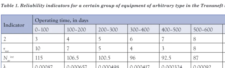
It is known that one type of equipment was in operation at Transneft PJSC, totalling 180 units, from 2006 to 2010. In this period, numbers of failures were established at certain intervals of operating time, and the following reliability indicators were determined: probability of failure-free work, failure rate. The results of this analysis are presented in Table 1.
Number of failures should be determined for a certain batch of equipment of the same type, 120 units of which were brought into operation in 2011. It is known that during the 0-100 operating days, ten equipment failures occurred (the number of failures in the following intervals of operating time is also presented in the table as rint with values Navint and λint corresponding to them, aiming to make it possible to compare results in the future).
The calculation will be performed for up to 700 days of the operating time of the equipment. The average value of equipment failure rate corresponds
t t r t N t r t t
N t t r t
i i
i i i i
i i i
0
1
0
1
2 = +
−
−
⋅
−
−
−
( ) ( )
( ) ∆
∆
∆
λ
ii
i i i
N r t r t
2
2
2
1
2
− − ( )∆ + ( )∆
(4b)
Indicator
Operating time, in days
0–100 100–200 200–300 300–400 400–500 500–600 600–700 700–800 800–900
2 3 4 5 6 7 8 9 10 11
r(Dt) 12 8 6 4 3 8 9 10 13
r(t) 12 20 26 30 33 41 50 60 73
Nav 174 164 169 172 174.5 173 167.5 166 163.5
P 0.93 0.88888 0.8555 0.8333 0.8166 0.7722 0.7222 0.6666 0.5944
λ 0.01 0.00049 0.0004 0.0002 0.0002 0.0005 0.0005 0.0006 0.0008
Indicator Operating time, in days
0–100 100–200 200–300 300–400 400–500 500–600 600–700
2 3 4 5 6 7 8 9
rint 10 7 5 4 3 8 11
Navint 115 106.5 100.5 96 92.5 87 77.5
λint 0.00087 0.000657 0.000498 0.000417 0.000324 0.00092 0.001419
r(Dt)’ 10 5.041051 3.850539 2.583146 1.953224 5.373318 5.918806
r(Dt) 10.58811 5.628682 4.522089 3.187314 2.530042 7.236001 8.231729 Table 1. Reliability indicators for a certain group of equipment of arbitrary type in the Transneft system.
to this operating time. The results of the calculation are presented in Table 2. Figure 6 compares the dynamics of predicted failures with target data at stages of operating time.
Under the conditions of this example, the total number of failures for equipment of this type in the operating time period from 0 to 700 hours was 48. As a result of primary analysis, the value equal to 34.72 was calculated. The corrected value, based on the probability of failure and on the average level of failure rate, was equal to 41.924. Thus, the proposed mathematical model enables evaluating the number of failures for specific technological unites of equipment and individual batches with maximum error of up to 15% (with an average error in the model of 4.5%). It is also worth noting that refining Equn 3 makes it possible to increase the calculation accuracy by approximately 20%.
Conclusions
At present, there is a considerable number of latent factory failures of equipment at production facilities of the oil and gas industry (based on the authors’ estimate,
the proportion of failures due to latent factory defects comprises around 32.5% of the total quantity of failures for equipment operating in the Transneft system). Correspondingly, measures aimed at creating and subsequently using industry-wide systems to assess product conformity to established requirements are fundamental measures for managing the reliability of the equipment. It should be noted that Transneft PJSC is one of the foremost organizations in this sector, and the corporate system of conformity assessment is implemented at all production facilities within organizations in the Transneft system. Due to the established tendency for optimizing the resources used in production (including during equipment inspection), the basis of the corporate system of conformity assessment is made up of various methods and methodologies for probability prediction of the condition of equipment. However, the probabilistic-statistical approach is an essentially new step in resolving this issue in Russian and international practice, therefore R&D studies in this area are particularly important and relevant at the moment.
The approaches developed and described in this article to making a quantitative
Indicator
Operating time, in days
0–100 100–200 200–300 300–400 400–500 500–600 600–700 700–800 800–900
2 3 4 5 6 7 8 9 10 11
r(Dt) 12 8 6 4 3 8 9 10 13
r(t) 12 20 26 30 33 41 50 60 73
Nav 174 164 169 172 174.5 173 167.5 166 163.5
P 0.93 0.88888 0.8555 0.8333 0.8166 0.7722 0.7222 0.6666 0.5944
λ 0.01 0.00049 0.0004 0.0002 0.0002 0.0005 0.0005 0.0006 0.0008
Indicator Operating time, in days
0–100 100–200 200–300 300–400 400–500 500–600 600–700
2 3 4 5 6 7 8 9
rint 10 7 5 4 3 8 11
Navint 115 106.5 100.5 96 92.5 87 77.5
λint 0.00087 0.000657 0.000498 0.000417 0.000324 0.00092 0.001419
r(Dt)’ 10 5.041051 3.850539 2.583146 1.953224 5.373318 5.918806
r(Dt) 10.58811 5.628682 4.522089 3.187314 2.530042 7.236001 8.231729
Operating time of the equipment, in hours
N
umber of eq
uipment f
ailur
es
Target number of failures
Predicted number of failures
prediction of equipment failures may be introduced into the current system of conformity assessment, given that over the past decade a sufficient quantity of statistical data has been collected about the equipment functioning at Transneft PJSC. Using probability-based methods of prediction makes it possible to improve the current systems of equipment inspection and, consequently, to increase its failure-free operation, conservability, and general operational readiness (by ‘general operational readiness’ the authors understand the characteristic of the equipment, which is described by basic integrated reliability indicators: the coefficient of readiness and the utilization rate).
References
1. O.V.Aralov, Yu.V.Lisin, and
B.N.Mastobaev, 2017. Methodological principles for managing product quality using conformity assessment mechanisms in trunk pipeline transportation. Monograph. St Petersburg: Nedra, p 350. 2. O.V.Aralov, 1999. A methodology for
optimising the planning of research and engineering work in technical means, communication systems, and automization, when using programmed planning. Dissertation for Cand. Sci. (Eng.) St Petersburg: MAC, p 285.
3. O.V.Aralov and A.V.Babkin, 1997.
Problems in optimising the planning of research and engineering works in communications technology: deposited manuscript. M. : CMRI MoD RF.
4. O.V.Aralov snd A.V.Babkin, 1997.
The basis for the optimization task in planning research and engineering works in communications technology. St Petersburg, p 20.
5. O.V.Aralov and A.V.Babkin, 1997. An analysis of methods and the current condition of solving the optimization task in planning research and engineering works in communications technology. St Petersburg, p 28.
6. O.V.Aralov, I.V.Buyanov, B.N.Mastobaev, N.V.Berezhansky, and D.V.Bylinkin, 2016. The main statements of optimization methodology of life-cycle parameters of process equipment. Science & Technologies: Oil and Oil Products Pipeline Transportation, 16 (6) pp23–29.
7. O.V.Aralov, D.V.Bylinkin, and
N.V.Berezhansky, 2016. Developing a methodological apparatus for calculating the probability of a defect appearing in equipment during its manufacture on the basis of the linear-dynamic programming method. Pipeline transportation. Material XI, International Scientific Research and Practice Conference, Ufa: USOTU publishers, 2016. pp 12-14.
8. O.V.Aralov et al., 2016. Determining
the optimal time for qualification testing of pumping-power equipment. Pipeline Transportation: Material XII, International Scientific Research and Practice Conference, Ufa: USOTU publishers, 2017. pp 126-129.
9. E.Y.Barzilovich., Y.K.Belyaev,
V.A.Kashtanov, I.N.Kovalenko, A.D.Solovyev, and I.A.Ushakov, 1983.
Aspects of Mathematical Theory of Reliability. B.V.Gnedenko, editor. Moscow (M): Radio i Svyaz, p 376.
10. R.E.Barlow aaand F.Proschan, 1960.
Mathematical theory of reliability. Moscow: Soviet Radio, p 488.
11. M.G.Kendall and A.Stuart, 1976.
Multivariate statistical analysis and time series. Moscow (M): Nauka; p 736. 12. A.I.Kobzar, 2006. Applied mathematical
statistics for engineers and scientists. Moscow (M): Fizmatlit, p 816.
13. Y.V.Lisin, O.V.Aralov, B.N.Mastobaev, N.V.Berezhansky, and D.V.Bylinkin, 2016. Development of a mathematical model for evaluating financial feasibility of the R&D plan for creation of complex technical systems. Transport and storage of oil products and hydrocarbons (3) pp17–23.
14. Y.V.Lisin, O.V.Aralov, B.N.Mastobaev, N.V.Berezhansky, and D.V.Bylinkin, 2016. Development of mathematical model for parameters optimization of R&D plan at homogeneous groups of technological
equipment. Transport and storage of oil