Feeding Ecology of Four Demersal Shark Species (Etmopterus spinax, Galeus melastomus, Scyliorhinus canicula and Squalus blainville) from the Eastern Aegean Sea

Turk. J. Fish.& Aquat. Sci. 19(6), 475-484 http://doi.org/10.4194/1303-2712-v19_6_03

Published by Central Fisheries Research Institute (SUMAE) Trabzon, Turkey in cooperation with Japan International Cooperation Agency (JICA), Japan

R E S E A R C H P A P E R

Feeding Ecology of Four Demersal Shark Species (

Etmopterus

spinax, Galeus melastomus, Scyliorhinus canicula

and

Squalus

blainville

) from the Eastern Aegean Sea

Fethi Bengil

_{* , Elizabeth G.T. Bengil}

_{, Sinan Mavruk}

_{, Ogulcan Heral}

_{, Ozan D.}

Karaman

_{, Okan Ozaydin}

1 _{Girne American University, Marine School, University Drive, PO Box 5, 99428 Karmi Campus, Karaoglanoglu, Girne, TRNC via}

TURKEY

2 _{Faculty of Fisheries, Ege University, P. O. Box 35100 Izmir, TURKEY}

3 _{Mediterranean Conservation Society, Doğa Villaları P.O. Box 35430 Izmir, TURKEY} 4 _{Çukurova University, Fisheries Faculty, P.O. Box 01330, Balcali/Adana TURKEY}

Article History

Received 22 February 2018 Accepted 01 June 2018 First Online 13 June 2018

Corresponding Author

Tel.: +90.392.6502000/1331 E-mail: fethibengil@gau.edu.tr

Keywords

Elasmobranches Diet composition Niche overlap Trophic level

The Eastern Mediterranean

Abstract

In this study, the diet composition and trophic ecology of four demersal chondrichthyan species; Etmopterus spinax, Galeus melastomus, Scyliorhinus canicula

and Squalus blainville were studied in the eastern Aegean Sea. In the stomachs of the samples which mostly consisted of juvenile individuals, a total of 97 prey taxa were identified. Teleost fishes were the most important prey group. The diversity of stomach content ranged between 15 species in E. spinax. and 70 species in S. canicula. The dietary breadth of G. melastomus and S. canicula were found to be narrower than the other two species examined. In addition, high niche overlap scores were detected amongst the species. All of the examined species had trophic levels higher than 4; with the highest trophic level being 4.20 and belonging to E. spinax. Comparisons among calculated trophic levels by global methods and a regional weighted method, which is proposed in this study, showed that the regional method offers remarkable advantages that can be used to reduce the uncertainty of the estimations.

Introduction

The effects of changes in either one or more components within a food web may propagate through the entire system, resulting in changes in the abundance and web connectivity of other species (Bornatowski, Wosnick, do Carmo, Corrêa, & Abilhoa, 2014). Considering the ongoing changes in many elasmobranch populations worldwide, and the potential impacts on their prey and communities, developing an understanding of trophic relationships of elasmobranches is important to comprehend how marine systems are functioning (Vaudo, 2011).

It is known that about 88 cartilaginous species inhabit the Mediterranean Sea (FAOa, 2018; FAOb, 2018), and that 75% of these species are also found in the Aegean Sea (Eronat & Bizsel, 2015). This group contributes a considerable part of by-catch in Turkish

trawl fisheries (Gurbet, Akyol, Yalçın, & Özaydın, 2013; Soykan, Akgül, & Kınacıgil, 2016). According to Eronat and Özaydın (2011) at least 15 chondrichthyan species are regularly presented in the fishery of study area. Four shark species investigated in this study: velvet belly lantern shark Etmopterus spinax (Linneus, 1758), blackmouth catshark Galeus melastomus Rafinesque, 1810, lesser spotted dogfish Scyliorhinus canicula

(Linneus, 1758), andlongnose spurdog Squalus blainville

(Risso, 1826), are among frequently caught elasmobranches in the Aegean Sea (Maravelias, Tserpes, Pantazi, & Peristeraki, 2012).

476

northern Atlantic (Ellis, Pawson, & Shackley, 1996), while in the western Mediterranean it also consumes polychaetas, teleosts and euphosid (Valls, Quetglas, Ordines, & Moranta, 2011). In general terms these same groups are also among the important food items for E. spinax (Bello, 1998; Fanelli, Rey, Torres, & Gil De Sola, 2009; Valls et al., 2011) and G. melastomus

(Anastasopoulou et al., 2013; Valls et al., 2011; Fanelli et al., 2009; Özütemiz, Kaya, & Özaydın, 2009; Serena et al., 2009 and references therein). To better understand sharks’ trophic ecology, further studies are required from different parts of the Mediterranean Sea and its adjacent waters (Stergiou & Karpouzi, 2001; Neves, Figueiredo, Moura, Assis, & Gordo, 2007; Albo-Puigserver et al., 2015; Kousteni, Karachle, & Megalofonou, 2017a).

The aim of this study was to develop an understanding on the trophic ecology of four demersal elasmobranch species: E. spinax, G. melastomus, S. canicula and S. blainville. For this purpose, diet composition was identified, niche breadth, diet overlaps and trophic levels were estimated, and their ecological significances were subsequently compared and discussed for each species.

Materials and Methods

Samples belonging to four elasmobranch species:

E. spinax, G. melastomus, S. canicula and S. blainville

were collected with a commercial bottom trawler. A total of 15 hauls were performed in 2008 (April, May, June, September and November) and 3 hauls were performed in 2014 (April), at depths between 150 and 550 m, off Sigacik Bay (26.569 N - 37.939 E and 26.879

N - 38.180 E), located in the eastern Aegean Sea (the eastern Mediterranean Sea) (Figure 1). A total of 2,174 specimens were collected and transported to the laboratory in a 4-8% formaldehyde solution. Total length and weights of individuals were measured and weighted to the nearest 0.1 cm and 0.01g using a measuring tape and electronic scale, respectively.

All prey items found in the stomach contents were identified to the lowest possible taxonomic level. Each prey item was weighed and recorded to the nearest 0.01 g using an electronic scale.

Analyses on diet comparisons were made between species. To evaluate the importance of each prey item, the percentage by number (N%), percentage by weight (W%), frequency of occurrence (FO%) and percentage index of relative importance (IRI%) were calculated (Hyslop, 1980) (see Eq. 1-5). For each species, percentage of empty stomachs were calculated from the ratio between the number of stomachs without prey items, and the total individuals examined.

Ni% = Ni

∑n_i=1N_i100 (1)

Wi% = W_i ∑ni=1Wi

100 (2)

FOi% = F_i

S100 (3)

IRIi= Fi%(Wi% + Ni%) (4)

IRIi% = IRIi

∑n_i=1IRI_i100 (5)

477

Where Ni is number of individual in prey category

i; Wi is weight of prey category i; Fi is number of

stomachs containing prey items in category i; S is the total number of full stomachs; IRIi is index of relative

importance of prey category i; n is the number of prey categories.

Cluster analysis was applied on the stomach contents of each examined species by using Euclidean distance with single linkage in order to evaluate similarities among feeding strategies.

Smith’s (1982) index (Eq. 6) was chosen to assess the niche breadth for two main reasons. Firstly, this method takes into account the availability of prey groups, and secondly it is less sensitive to the selectivity of lesser important prey groups (Krebs, 2009).

FT = Σ(√aipi) (6)

Where FT is Smith’s (1982) index; pi is the

proportion of individuals using prey category i; ai is IRI%

of prey category i to the total prey composition. Levins’ measure of niche breadth (Eq. 7) and Levins’ standardized niche breadth were (Eq. 8) also calculated (Krebs, 2009).

B ̂ = 1

Σpi2

⁄ (7)

B

̂_A=(B̂ − 1)

(n − 1)

⁄ (8)

Where 𝐵̂ is Levins’ measure of niche breadth; 𝐵̂𝐴 is Levins’ standardized niche breadth; and n is the number of prey categories.

Due to the various sample sizes, Morisita index was chosen to calculate niche overlap among the investigated species by using main taxa to avoid bias as suggested by Krebs (2009) (Eq. 9).

𝐶 = 2 ∑ 𝑝𝑖𝑗𝑝𝑖𝑘

𝑛 𝑖

∑ 𝑝𝑖𝑗[

(𝑛𝑖𝑗−1)

(𝑁_𝑗−1)

⁄ ]+∑ 𝑝_𝑖𝑘[(𝑛𝑖𝑘−1)

(𝑁_𝑘−1)

⁄ ]

𝑛 𝑖 𝑛

𝑖

(9)

Where C is Morisita’s index of niche overlap between species j and k; pij is the proportion of

individuals using prey category i. to total prey composition used by species j; pik is the proportion of

individuals using prey category i to the total prey composition used by species k; nij is the number of

individuals of species j that used prey category i; nik is

number of individuals of species k that used prey category i; Nj and Nk are the total number of species j

and k, respectively.

According to the contribution of each taxon from different groups, trophic levels of the prey groups were adapted based on local prey composition. When available, the trophic level of each identified species was taken from FishBase (http://www.fishbase.org, Froese

& Pauly, 2016) or SeaLifeBase

(http://www.sealifebase.org, Palomares & Pauly, 2017). When the trophic levels were not available, group values were used from Pauly et al., (2000) or from Ebert and Bizzarro (2007) and the references therein. Following

Table 1. Standardized diet compositions and their trophic levels for the Aegean Sea

Group code Description Trophic level

AMPH Amphipods and isopods 3.18

CEPH Octopi, cuttlefishes and unidentified cephalopods 3.21

CHOND Chondrichthyan fishes 3.78

DECA Decapods 2.93

EUPH Euphausiids and mysids 2.25

FISH Teleost and agnathan fishes 3.26

INVERT Other invertebrates and unidentified invertebrates 2.17 MOLL Mollusk (excluding cephalopods) and unidentified mollusks 2.10 OCRUST Other crustaceans and unidentified crustaceans 2.60

POLY Polychaetes and other marine worms 2.30

SQUID Squids 4.06

Table 2. Total number of sampled specimens from each shark species (N), number of stomachs with food (N of FS), percentage of

empty stomachs (PES), range and averages of length (L), and average of weight (W) measurements

Species N N of FS PES Range L

(mm)

Average L (mm)

Average W (g)

Etmopterus spinax 129 97 25% 86-317 171 28

Galeus melastomus 441 336 24% 89-450 152 17

Scyliorhinus canicula 1296 241 81% 44-512 198 54

Table 3. Standardized diet compositions and percentage index of relative importance for each shark species

Etmopterus spinax Galeus melastomus Scyliorhinus canicula Squalus blainville

Group Taxon Fo% N % W % IRI IRI % Fo% N % W % IRI IRI % Fo% N % W % IRI IRI % Fo% N % W % IRI IRI %

AMPH

Amphipoda 1.05 0.81 0.05 0.91 0.02 0.28 0.23 0.01 0.07

Isopoda 1.13 0.93 0.20 1.28 0.04 0.26 0.21 0.08 0.07 0.01 AMPH 1.05 0.81 0.05 0.91 0.02 1.41 1.17 0.22 1.95 0.03 0.26 0.21 0.08 0.07 0.00

CEPH

Cephalopoda 36.84 45.53 38.95 3112.37 74.41 5.63 4.44 3.71 45.93 1.59 10.26 9.17 4.91 144.34 10.07 6.02 6.04 17.97 144.66 6.58

Octopodidae 0.28 0.23 0.02 0.07 0.26 0.21 0.05

Pteroctopus tetracirrhus 0.26 0.21 2.93 0.80 0.06

Sepia officinalis 0.26 0.21 0.13 0.09 0.01

Sepia orbignyana 0.26 0.21 0.04 0.06

Sepia sp. 0.51 0.42 0.39 0.41 0.03

Sepietta neglecta 0.26 0.21 0.33 0.14 0.01

Sepietta oweniana 0.26 0.42 0.84 0.32 0.02

Sepietta sp. 1.05 0.81 2.35 3.33 0.08 1.79 1.46 1.90 6.03 0.42 1.20 1.65 1.30 3.55 0.16

Sepiolidae 1.41 1.17 1.05 3.12 0.11 0.77 1.04 1.71 2.11 0.15 1.20 1.10 1.50 3.13 0.14 CEPH 37.89 46.34 41.30 3321.22 58.73 7.32 5.84 4.78 77.82 1.12 14.87 13.54 13.18 397.34 8.62 8.43 8.79 20.77 249.28 5.59

CHOND

Chondrichthyes 0.60 0.55 0.76 0.79 0.04

Raja sp. 0.28 0.23 0.08 0.09

Scyliorhinus canicula 0.51 0.42 0.81 0.63 0.04

CHOND 0.28 0.23 0.08 0.09 0.00 0.51 0.42 0.81 0.63 0.01 0.60 0.55 0.76 0.79 0.02

DECA

Alpheus sp. 0.77 0.63 0.67 1.00 0.07 1.20 1.10 0.28 1.66 0.08

Aristeomorpha folicea 0.56 0.47 0.15 0.35 0.01 0.51 0.42 1.14 0.80 0.06

Brachyura 0.26 0.21 0.14 0.09 0.01 0.60 0.55 0.33 0.02

Chlorotoccus crassicornis 0.26 0.21 0.01 0.06

Galathea sp. 0.26 0.21 0.01 0.06

Goneplax rhomboides 0.26 0.42 0.19 0.16 0.01

Macropipus sp. 0.26 0.21 0.03 0.06

Munida rutllanti 0.77 0.63 0.86 1.14 0.08 0.60 0.55 0.12 0.40 0.02

Natantia 2.82 2.34 1.21 10.00 0.35

Pagurus sp. 0.26 0.21 0.06 0.07 0.60 0.55 0.15 0.42 0.02

Panaediae 0.28 0.23 0.07 0.09

Pandalus sp. 0.28 0.23 0.22 0.13

Parapenaeus longirostris 0.56 0.47 0.29 0.43 0.01 8.46 9.58 11.86 181.48 12.66 5.42 5.49 5.70 60.71 2.76

Parthenope massana 0.26 0.21 0.16 0.09 0.01

Pasiphea sivado 6.32 5.69 2.44 51.37 1.23

Penaeus kerathurus 2.05 2.08 2.26 8.91 0.62

Philocheras sp. 0.28 0.23 0.04 0.08

Plesionika edwarsi 3.59 3.33 1.15 16.09 1.12

Plesionika martia 1.05 0.81 1.61 2.55 0.06

Plesionika sp 5.35 4.91 4.37 49.65 1.72 2.05 2.08 2.02 8.43 0.59 2.41 3.30 1.00 10.36 0.47

Pontocaris sp. 0.28 0.23 0.05 0.08 0.26 0.21 0.08 0.07 0.01 0.60 0.55 0.11 0.40 0.02

Processa sp. 1.05 0.81 0.31 1.18 0.03 1.03 0.83 0.41 1.27 0.09 1.20 1.10 0.19 1.56 0.07

Solenocera membranacea 0.85 1.17 0.39 1.31 0.05 0.26 0.21 0.11 0.08 0.01 0.60 0.55 0.28 0.50 0.02

Synalpheus sp. 0.51 0.42 0.11 0.27 0.02 0.60 0.55 0.05 0.36 0.02

DECA 8.42 7.32 4.37 98.38 1.74 11.27 10.28 6.80 192.45 2.77 22.05 22.08 21.27 955.93 20.74 13.86 14.29 7.89 307.26 6.89

EUPH

Euphasiacea 0.26 0.21 0.06 0.07

Mysidacea 3.16 6.50 0.22 21.24 0.51 9.58 21.50 1.14 216.77 7.51 7.18 15.63 0.94 118.96 8.30 2.41 3.85 0.06 9.42 0.43 EUPH 3.16 6.50 0.22 21.24 0.38 9.58 21.50 1.14 216.77 3.13 7.44 15.83 1.01 125.21 2.72 2.41 3.85 0.06 9.42 0.21

FISH

Antonogadus megalokynodon 1.20 1.10 0.77 2.25 0.10

Argentina sphyraena 0.28 0.23 0.11 0.10 2.31 1.25 3.11 10.05 0.70 1.81 1.65 1.74 6.13 0.28

Arnoglossus laterna 0.51 0.42 1.75 1.11 0.08

Arnoglossus rueppelli 0.51 0.42 0.21 0.32 0.02

Buglossidium luteum 0.26 0.21 1.22 0.37 0.03

Capros aper 0.26 0.21 0.09 0.08 0.01

Chlorophtalmus agassizi 1.41 1.17 1.34 3.54 0.12

Citharus linguatula 0.26 0.21 2.57 0.71 0.05

Clupeidae 0.26 0.21 0.02 0.06

478

Tu

rk.

J.

Fis

h

.&

Aq

u

a

t.

S

ci. 19(

6

),

475

-48

Table 3. Continued

Diplodus annularis 0.26 0.42 2.50 0.75 0.05

Engraulis encrasicholus 0.51 0.42 1.46 0.96 0.07

Gadella maraldi 0.56 0.47 0.47 0.53 0.02

Gadiculus argenteus 0.28 0.23 0.20 0.12 3.08 3.54 6.81 31.86 2.22 4.22 3.85 4.45 34.98 1.59

Glossanodon leioglossus 1.20 1.10 3.86 5.97 0.27

Gnathophis mystax 0.51 0.42 1.94 1.21 0.08 0.60 0.55 6.06 3.98 0.18

Gobius niger 0.26 0.21 1.22 0.37 0.03

Gonostoma denudatum 1.05 0.81 0.70 1.59 0.04

Hymenocephalus italicus 0.85 0.70 0.58 1.09 0.04 1.03 0.83 1.75 2.65 0.19 1.20 1.10 0.29 1.67 0.08

Lampanyctus crocodilus 0.85 0.70 1.30 1.69 0.06 0.26 0.21 0.18 0.10 0.01

Lesueurigobius friesii 0.51 0.42 0.47 0.46 0.03

Macrouridae 2.54 2.10 37.97 101.59 3.52 1.20 1.10 0.57 2.01 0.09

Merluccius merluccius 0.51 0.42 2.05 1.26 0.09 0.60 0.55 3.30 2.32 0.11

Myctophidae 11.58 8.94 16.47 294.30 7.04 7.32 7.01 9.82 123.29 4.27 1.54 1.67 4.26 9.12 0.64 0.60 0.55 0.22 0.47 0.02

Nezumia sp. 0.56 0.47 1.02 0.84 0.03

Phycis blennoides 0.26 0.21 0.03 0.06 1.20 1.10 4.04 6.20 0.28

Phycis phycis 0.28 0.23 0.71 0.27 0.01

Pleuronectiformes 0.6 0.55 0.53 0.65 0.03

Scorpaenidae 0.26 0.21 0.71 0.23 0.02

Teleostei (Unidentified) 16.84 13.01 13.90 453.22 10.84 34.08 30.14 26.30 1923.80 66.67 21.03 18.75 19.07 795.17 55.49 21.08 19.23 17.46 773.53 35.20

Trachinus draco 0.26 0.21 0.05

Vinciguerria attenuata 2.11 2.44 6.44 18.70 0.45

Zeus faber 0.26 0.21 0.15 0.09 0.01

FISH 31.58 25.20 37.52 1980.77 35.02 49.01 43.46 79.84 6043.33 87.12 34.87 31.04 51.57 2880.86 62.50 35.54 32.42 43.29 2690.78 60.34

INVERT

Actinaria (Unidentified) 0.26 0.21 0.61 0.21 0.01

Anthozoa (Unidentified) 1.20 3.30 0.24 4.27 0.19

Antodon mediterranea 0.51 0.42 0.03 0.23 0.02 1.20 1.10 0.59 2.04 0.09

Echinodermata 0.26 0.21 0.05 0.07

Hexacorallia 0.28 0.23 0.02 0.07

Siphonophora 0.26 0.21 0.30 0.13 0.01

Tunicata 1.05 0.81 5.07 6.19 0.15 0.26 0.42 1.22 0.42 0.03

INVERT 1.05 0.81 5.07 6.19 0.11 0.28 0.23 0.02 0.07 0.00 1.54 1.46 2.22 5.65 0.12 2.41 4.40 0.84 12.61 0.28

MOLL Bivalvia (Unidentified) 0.26 0.21 0.01 0.05

MOLL 0.26 0.21 0.01 0.05 0.00

OCRUST

Crustacea (Unidentified) 14.74 11.38 2.49 204.50 4.89 18.87 15.65 5.41 397.46 13.77 6.15 5.00 1.37 39.18 2.73 28.31 27.47 10.31 1069.71 48.67

Cumacean 0.51 0.63 0.01 0.32 0.02

Squilla mantis 3.33 2.71 2.89 18.65 1.30

Squilla massavensis 0.77 0.63 1.61 1.72 0.12

Squilla sp. 2.05 1.88 0.65 5.19 0.36

OCRUST 14.74 11.38 2.49 204.50 3.62 18.87 15.65 5.41 397.46 5.73 12.82 10.83 6.53 222.56 4.83 28.31 27.47 10.31 1069.71 23.99 POLY Polycheata (Unidentified) 3.08 2.50 1.65 12.78 0.89 3.01 3.30 1.98 15.89 0.72

POLY 3.08 2.50 1.65 12.78 0.28 3.01 3.30 1.98 15.89 0.36

SQUID

Abralia veranyi 0.56 0.47 0.17 0.36 0.01 0.77 0.63 0.12 0.57 0.04

Allouteuthis media 0.28 0.23 0.05 0.08

Allouteuthis sp. 0.60 0.55 0.58 0.68 0.03

Allouteuthis subulata 0.26 0.21 0.45 0.17 0.01

Heteroteuthis dispar 0.56 0.47 0.54 0.57 0.02

Illex coindetii 1.05 0.81 2.81 3.81 0.09 0.26 0.21 0.08 0.07 0.01 2.41 2.20 5.50 18.54 0.84

Loligo vulgaris 1.03 0.83 1.05 1.93 0.13 1.20 1.10 2.42 4.24 0.19

Pyroteuthis margoritifera 0.56 0.47 0.95 0.80 0.03

Todarodes sagittatus 1 1 6 7 0 1 1 4 3 0

Todaropsis eblanea 0.6 0.55 1.36 1.15 0.05

SQUID 2.11 1.63 8.98 22.32 0.39 1.97 1.64 1.72 6.62 0.10 2.31 1.88 1.69 8.23 0.18 5.42 4.95 14.11 103.30 2.32

479

Tu

rk.

J.

Fis

h

.&

Aq

u

a

t.

S

ci. 19(

6

),

475

-48

480

from this stage, all taxa found in the examined stomachs were then classed as the prey categories of Ebert and Bizzarro (2007). IRI% was used to calculate the proportional contribution of each taxon within a group. The contribution of each taxon and their trophic levels were then used to calculate the weighted average trophic level of each standardized prey group (Table 1). Afterwards, trophic levels of examined species (TL) were calculated by using Equation 10.

TL = 1 + (∑𝑛𝑗=1(𝐼𝑅𝐼%)𝑗∗ 𝑇𝐿𝑗) (10)

Where TLj is the trophic level of each prey category

j; IRI%j is the percentage in index of relative importance

per prey category j.

In addition, the trophic level values of each species were also estimated by using the methods of Ebert and Bizzarro (2007) as well as Cortés (1999) in order to compare both local and global trophic levels.

Results

Stomach Contents

During the study period a total of 2,174 specimens belonging to four investigated species were sampled. The total number of full stomachs were 97, 166, 241 and 336 for E. spinax, S. blainvillei, S. canicula, and G. melastomus, respectively. The lowest empty stomach percentage (24%) was observed in G. melastomus,with the highest percentage (81%) found in S. canicula (Table 2). The number of examined stomachs and descriptive statistics of the length measurements of each shark species are also given in Table 2. A total of 97 prey taxa were identified in the study, and all identified taxa were classified under 11 categories according to their trophic

levels. The diet diversity was discovered to be highest in

S. canicula with a total of 70 taxa (in 11 groups), and lowest in E. spinax with 15 taxa (in 8 groups). G. melastomus and S. blainville fed on 33 and 36 taxa belonging to 9 groups, respectively (Table 3).

The main prey taxa consumed by E. spinax were cephalopods and teleost fishes. More specifically, Myctopids and unidentified crustaceans were found to constitute an important part of the diet. The contributions of species from other prey groups were considered to be negligible (Table 3).

Teleost fishes were also identified as being dominant in the diet of G. melastomus. While unidentified teleost species showed the highest contribution to IRI%, the contributions of Macrouridae and Myctophidae were also relatively higher than other groups. Unidentified crustaceans and mysids (in the euphasiid group) were other important food items, with IRI% more than 5%(Table 3).

Although the stomach contents of S. canicula and

S. blainville showed similar compositions (Figure 2), the IRI ratios of main prey taxa showed differences between the species. Results from S. canicula displayed unidentified teleost species as their dominant prey. On the other hand, this same group of teleost species were also the second dominant prey group for S. blainville.

Relatively important prey species was a teleost,

Gadiculus argentatus, along with Parapenaus longirostris, Unidentified Crustaceans and Cephalopods in the diets of both species (Table 3).

Niche Breath, Niche Overlap and Trophic Level

Smith’s (1982) index for niche breadth indicated that the dietary breadths of G. melastomus and S. canicula were narrower than the other two examined

Figure 2. Cluster analysis dendogram of the examined species based on Euclidian similarity distance of their diets.

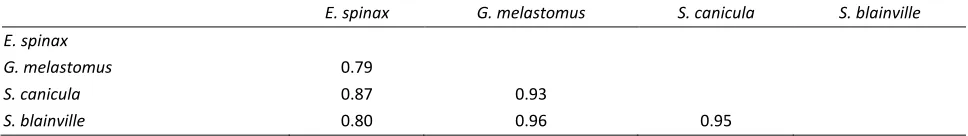
Table 4. Morisita’s niche overlap values among the species. All values show significant overlap between the species

E. spinax G. melastomus S. canicula S. blainville E. spinax

G. melastomus 0.79

S. canicula 0.87 0.93

481

species, with the highest index score was seen in S. blainville. In addition to Smith’s (1982) index, Levins’ measures of niche breadth ranged from 3.65 (E. spinax) to 4.63 (S. canicula) and Levins’s standardized niche breadth ranged from 0.29 (G. melastomus) to 0.40 (S. blainville) (Figure 3).

The results of Morisita’s niche overlap analysis amongst the species showed that the maximum level in overlap was observed between S. blainville and G. melastomus (0.96). Niche overlaps between S. blainville – S. canicula, and S. canicula – G. melastomus were determined at

0.95 and 0.93, respectively (Table 4). The least overlap was detected between E. spinax and the other examined species. The overlap analyses indicated that the food tendencies of four species were considerably similar to each other.

The trophic levels of examined species ranged from 4.08 (S. blainville) to 4.20 (E. spinax) with an average value of 4.15±0.6 (±standard deviation, n=4). Trophic level calculations using global methods were given in Table 5.

Discussion

Stomach Content

In accordance with previous studies in adjacent regions from Mediterranean Sea, teleosts fishes, crustaceans and cephalopods are the main prey groups for the four shark species examined here, though their relative importance changes (Bello, 1998; Kabasakal, 2002; Olaso et al., 2005; Neves et al., 2007; Fanelli et al.,

2009; Özütemiz et al., 2009; Serena et al., 2009 and references therein; Valls et al., 2011; Anastasopoulou et al., 2013; Kousteni et al., 2017a; Kousteni et al., 2017b;). Parallel to our findings on main prey groups, the distribution of length measurements of samples collected in this study showed narrow ranges. Information on size at maturity of each species from previous studies also supports most of the examined specimens (85% of S. canicula individuals were immature, lowest among other species) were juveniles (see Metochis, Carmona-Antoñanzas, Kousteni, Damalas, & Megalofonou, 2016 for G. melastomus; Porcu et al., 2014 for E. spinax; Kousteni, Kontopoulou, & Megalofonou, 2010 for S. canicula; Kousteni &

Figure 3. Scores of niche breadth from different approaches for each investigated species.

Table 5. Trophic levels of the species with weighted average of diet compositions and table values of Ebert and Bizzaro (2007) and

Cortés (1999).

Trophic Level

This study Approach of Ebert and Bizzaro (2007) Approach of Cortés (1999)

Etmopterus spinax 4.2 4.17 4.19

Galeus melastomus 4.18 4.14 3.64

Scyliorhinus canicula 4.12 4.02 4.11

Squalus blainville 4.08 3.98 3.98

3.65

3.29

4.63

4.2

0.38 _0.29 0.36 0.4

0.94 0.9 0.94 0.95

0 1 2 3 4 5

E. spinax G. melastomus S. canicula S. blainville

N I C H E BR E A D T H

482

Megalofonou, 2015 for S. blainville). Thus, our results may represent characteristics of mostly juveniles of these species.

Niche Breath, Niche Overlap, Trophic Level

Even though results on niche breadth indicated differences between the regions and studies (Ellis et al.,

1996; Fanelli et al., 2009; Valls et al., 2011), these findings should be interpreted with caution since these values may be biased due to the use of different approaches between studies. In this regard, Krebs (2009) suggested that the usage of the number of individuals gives a better result by comparisons to the usage of proportional prey items whilst calculating p values. Unlike the present study, the mentioned studies on niche breadth and overlap used proportions, and therefore this methodological deviation may explain the inconsistencies amongst studies.

Niche overlap had high values amongst the four shark species examined parallel to the results of stomach content analysis. Most similar stomach contents were observed between S. blainville and S. canicula, with these two species also showing one of the highest niche overlap. A similar significant overlap was observed between these species in the coasts of Portugal, in the Atlantic Ocean (Martinho et al., 2012).

The results of present study showed that the trophic levels of shark species examined in this study are between 4.08 and 4.2 and these values indicated that the species under consideration are tertiary consumers based on the definition of Cortés (1999). In addition, the examined species can also be classified under groups of carnivores, which Stergiou and Karpouzi (2001) defined the group as potential top carnivores in the

Mediterranean Sea. As the diet compositions of these demersal elasmobranch species showed a dominancy of benthic organisms, these sharks can be considered as representative of high level consumers in the demersal community of the Aegean Sea.

Findings from our trophic level comparisons showed that the trophic levels of the examined species are mostly higher in the eastern, rather than the western Mediterranean Sea (Table 6). This tendency can be an indicator of trophic structure in benthic ecosystems. Danovaro, Dinet, Duineveld, and Tselepides, (1999) reported eastern basin is subject to more limiting trophic conditions, and so may have had a higher efficiency in exploiting the particulate organic fluxes, opposed to the western Mediterranean Sea; with the higher trophic input in the western Mediterranean Sea being partially balanced by the higher trophic efficiency of the deep eastern Mediterranean Sea. Thus, results show clear differences in the trophic characteristics of the two environments.

Cortés (1999) points out that using weighted averages of diet compositions by different data-sets is a more accurate approach for trophic level calculation. Furthermore, using a standardized diet composition of sharks is practical for comparison purposes and better understanding their roles in ecosystems. Nonetheless, using standardized groups as a generalization brings some inherent bias for the estimation of trophic levels per examined species. For instance, the trophic level estimation of G. melastomus was found as 4.18 with locally weighted trophic level values of standardized diet composition, whilst it was found as 3.64 by using the method of Cortés (1999) and as 4.08 by using the method of Ebert and Bizzarro (2007). In contrast, some species, such as E. spinax, showed insignificant

Table 6. Trophic levels of the examined species from different studies and present study.

Species Reference Study area Trophic level

Etmopterus spinax

Cortés (1999) 3.8

Froese and Pauly (2016) 3.6

Stergiou and Karpouzi (2002) W Mediterranean 3.80-4.33 (Min-Max) Albo-Puigserver et al. (2013) W Mediterranean 3.71

This study E Aegean 4.20

Galeus melastomus

Froese and Pauly (2016) 3.8

Cortés (1999) 3.7

Stergiou and Karpouzi (2002) W Mediterranean 3.70-4.26 (Min-Max) Neves et al. (2007) S Portagual 4.02 Albo-Puigserver et al. (2013) W Mediterranean 4.17

This study E Aegean 4.18

Scyliorhinus canicula

Froese and Pauly (2016) 3.6

Cortés 1999 3.6

Stergiou and Karpouzi (2002) W Mediterranean 3.8 Pinnegar et al. (2002) Celtic Sea 4.29 Kousteni et al. (2017) C and W Aegean Sea 4.22

This study E Aegean 4.12

Squalus blainville

Froese and Pauly (2016) 3.6

Cortés (1999) 4

483

differences among the trophic level calculation methods (Table 5). Regional trophic level values for each standardized diet group should be used for reducing the uncertainty of the estimations, as faunal characteristics in a specific region can determine the species compositions of each standardized diet group. The relative contribution of each prey in the same group may significantly affect the value of trophic level. Global databases such as “FishBase” and “SeaLifeBase” make available trophic level values for most species. Simultaneously, most studies on stomach contents give information about prey items on species or genus level. When considering this availability, collections from studies in a certain region, such as the Aegean Sea or the eastern Mediterranean Sea, using local studies for calculation of weighted trophic level of each standardized diet composition, will give more accurate and comparable information either within a region or among regions.

Acknowledgement

Authors would like to thank Prof. Dr. Alp SALMAN for identification of cephalopod remains. Part of the study was supported by TUBITAK under the grant program 2209.

References

Albo-Puigserver, M., Navarro, J., Coll, M., Aguzzi, J., Cardona, L., & Sáez-Liante, R. (2015). Feeding ecology and trophic position of three sympatric demersal chondrichthyans in the northwestern Mediterranean. Marine Ecology Progress Series, 524, 255–268.

https://doi.org/10.3354/meps11188

Anastasopoulou, A., Mytilineou, C., Lefkaditou, E., Dokos, J., Smith, C.J., Siapatis, A., … Papadopoulou, K.N. (2013). Diet and feeding strategy of blackmouth catshark Galeus melastomus. Journal of Fish Biology, 83(6), 1637–1655. https://doi.org/10.1111/jfb.12269

Bello, G. (1998). The feeding ecology of the velvet belly,

Etmopterus spinax (Chondrichthyes: Squalidae), of the Adriatic Sea on the basis of its stomach contents. Atti Soc. It Sci. Nat. Museo Civ. Stor. Nat. Milano, 139(2), 187–193.

Bornatowski, H., Wosnick, N., do Carmo, W.P.D., Corrêa, M.F.M., & Abilhoa, V. (2014). Feeding comparisons of four batoids (Elasmobranchii) in coastal waters of southern Brazil. Journal of the Marine Biological Association of the United Kingdom, 94(7), 1491–1499. https://doi.org/10.1017/S0025315414000472

Cortés, E. (1999). Standardized diet compositions and trophic levels of sharks. ICES Journal of Marine Science, 56(5), 707–717.

https://doi.org/10.1006/jmsc.1999.0489

Danovaro, R., Dinet, A., Duineveld, G., & Tselepides, A. (1999). Benthic response to particulate fluxes in different trophic environments: a comparison between the Gulf of Lions–Catalan Sea (Western-Mediterranean) and the Cretan Sea (eastern-Mediterranean). Progress in Oceanography, 44(1–3), 287–312.

https://doi.org/10.1016/S0079-6611(99)00030-0 Ebert, D.A., & Bizzarro, J.J. (2007). Standardized diet

compositions and trophic levels of skates (Chondrichthyes: Rajiformes: Rajoidei). Environ. Biol. Fishes 80, 221–237. https://doi.org/10.1007/s10641-007-9227-4

Ellis, J.R., Pawson, M.G., & Shackley, S.E. (1996). The Comparative Feeding Ecology of Six Species of Shark and Four Species of Ray (Elasmobranchii) In the North-East Atlantic. Journal of the Marine Biological Association of the United Kingdom, 76(1), 89.

https://doi.org/10.1017/S0025315400029039

Eronat, E.G.T., & Bizsel, K.C. (2015). Diversity in Fish Fauna of Turkish seas. DEVOTES-EUROMARINE Summer School 9th to 11th June 2015 - Aquarium of Donostia- San Sebastián

Eronat, E.G.T., & Özaydın, O. (2011). Sığacık Körfezi’ndeki kıkırdaklı balık biyoçeşitliliği. 16. Su Ürünleri Sempozyumu 25-27 Ekim, 2011 Akdeniz Üniversitesi, Antalya.

FAOa, 2018. Species Photographic Plates. Mediterranean Sharks, by Monica Barone, Fabrizio Serena and Mark Dimech. Rome, Italy.

FAOb, 2018. Species Photographic Plates. Mediterranean skates, rays and chimaeras, by Monica Barone, Fabrizio Serena and Mark Dimech. Rome, Italy.

Fanelli, E., Rey, J., Torres, P., & Gil De Sola, L. (2009). Feeding habits of blackmouth catshark Galeus melastomus

Rafinesque, 1810 and velvet belly lantern shark

Etmopterus spinax (Linnaeus, 1758) in the western Mediterranean. Journal of Applied Ichthyology,

25(SUPPL. 1), 83–93.

https://doi.org/10.1111/j.1439-0426.2008.01112.x Froese, R., & Pauly, D. (2016). FishBase. World Wide Web

electronic publication.www.fishbase.org, version (01/2016).

Gurbet, R., Akyol, O., Yalçın, E., & Özaydın, O. (2013). Discards in bottom trawl fishery in the Aegean Sea (Izmir Bay, Turkey). Journal of Applied Ichthyology, 29(6), 1269– 1274.

https://doi.org/10.1111/jai.12243

Hyslop, E.J. (1980). Stomach contents analysis-a review of methods and their application. Journal of Fish Biology,

17(4), 411–429.

https://doi.org/10.1111/j.1095-8649.1980.tb02775.x Kabasakal, H. (2002). Stomach contents of the longnose

spurdog, Squalus blainvillei (Risso, 1826) from the north-eastern aegen sea. Annales, Series Historia Naturalis,

12(2), 173–176.

Kousteni, V., & Megalofonou, P. (2015). Aging and life history traits of the longnose spiny dogfish in the Mediterranean Sea: New insights into conservation and management needs. Fisheries Research, 168, 6-19.

Kousteni, V., Karachle, P.K., & Megalofonou, P. (2017a). Diet of the small-spotted catshark Scyliorhinus canicula in the Aegean Sea (eastern Mediterranean). Marine Biology Research, 13(2), 161–173. https://doi.org/10.1080/17451000.2016.1239019 Kousteni, V., Karachle, P.K., & Megalofonou, P. (2017b). Diet

and trophic level of the longnose spurdog Squalus blainville (Risso, 1826) in the deep waters of the Aegean Sea. Deep Sea Research Part I: Oceanographic Research Papers, 124, 93–102.

484

Kousteni, V., Kontopoulou, M., & Megalofonou, P. (2010). Sexual maturity and fecundity of Scyliorhinus canicula

(Linnaeus, 1758) in the Aegean Sea. Marine Biology Research, 6(4), 390-398.

Krebs, J.C. (2009). Ecological methodology (2nd ed.). New York: Addison Wesley Longman.

Maravelias, C.D., Tserpes, G., Pantazi, M., & Peristeraki, P. (2012). Habitat Selection and Temporal Abundance Fluctuations of Demersal Cartilaginous Species in the Aegean Sea (Eastern Mediterranean). PLoS ONE, 7(4), e35474. https://doi.org/10.1371/journal.pone.0035474 Metochis, C., Carmona-Antoñanzas, G., Kousteni, V., Damalas, D., & Megalofonou, P. (2016). Population structure and aspects of the reproductive biology of the blackmouth catshark, Galeus melastomus Rafinesque, 1810 (Chondrichthyes: Scyliorhinidae) caught accidentally off the Greek coasts. Journal of the Marine Biological Association of the United Kingdom, 1-17. doi:10.1017/S0025315416001764

Neves, A., Figueiredo, I., Moura, T., Assis, C., & Gordo, L. S. (2007). Diet and Feeding Strategy of Galeus melastomus

in the Continental Slope Off Southern Portugal. Vie et Milieu - Life and Environment, 57(3), 165–169.

Olaso, I., Velasco, F., Sánchez, F., Serrano, A., Rodríguez-Cabello, C., & Cendrero, O. (2005). Trophic Relations of Lesser-Spotted Catshark (Scyliorhinus canicula) and Blackmouth Catshark (Galeus melastomus) in the Cantabrian Sea. Journal of Northwest Atlantic Fishery Science, 35, 481–494. https://doi.org/10.2960/J.v35.m494

Özütemiz, Ş., Kaya, M., & Özaydın, O. (2009). Sığacık Körfezi’nde (Ege Denizi) Bulunan İki Tür Köpekbalığının [Galeus melastomus Rafinesque,1810 ve Squalus blainvillei (Risso, 1826)] Boy-Ağırlık İlişkisi ve Beslenme Özellikleri Üzerine Bir Ön Çalışma. EU. Journal of Fisheries & Aquatic Sciences, 26(3), 211–217.

Palomares, M.L.D., & Pauly, D. (2017). SeaLifeBase. World Wide Web electronic publication. www.sealifebase.org, version (01/2016).

Pauly, D., Froese, R., Sala, P.S., Palomares, M.L., Christensen, V., & Rius, J. (2000). Trophlab manual. ICLARM. Manila, Philippines.

Porcu, C., Marongiu, M.F., Follesa, M.C., Bellodi, A., Mulas, A., Pesci, P., & Cau, A. (2014). Reproductive aspects of the velvet belly lantern shark Etmopterus spinax

(Condrichthyes: Etmopteridae), from the central western Mediterranean Sea. Notes on gametogenesis and oviducal gland microstructure. Mediterranean Marine Science, 15(2), 313-326.

Serena, F., Mancusi, C., Ungaro, N., Hareide, N. R., Guallart, J., Coelho, R., & Crozier, P. (2009). Galeus melastomus. The IUCN Red List of Threatened Species 2009.

Smith, E.P. (1982). Niche Breadth Resource Availability, and Inference. Ecology, 63(6), 1675–1681.

Soykan, O., Akgül, Ş.A., & Kınacıgil, H.T. (2016). Catch composition and some other aspects of bottom trawl fishery in Sığacık Bay, central Aegean Sea, eastern Mediterranean. Journal of Applied Ichthyology, 32(3), 542–547. https://doi.org/10.1111/jai.13042

Stergiou, K.I., & Karpouzi, V.S. (2001). Feeding habits and trophic levels of Mediterranean fish. Reviews in Fish Biology and Fisheries, 11(3), 217–254. https://doi.org/10.1023/A:1020556722822

Valls, M., Quetglas, A., Ordines, F., & Moranta, J. (2011). Feeding ecology of demersal elasmobranchs from the shelf and slope off the Balearic Sea (western Mediterranean). Scientia Marina, 75(4), 633–639. https://doi.org/10.3989/scimar.2011.75n4633