Approximation of feedback linearization control input based on fuzzy wavelet networks

© Shiraz University

APPROXIMATION OF FEEDBACK LINEARIZATION CONTROL INPUT

BASED ON FUZZY WAVELET NETWORKS*

M. ZEKRI**_{, S. SADRI AND F. SHEIKHOLESLAM}

Dept. of Electrical and Computer Engineering, Isfahan University of Technology, I. R. of Iran Email: [email protected]

Abstract– Based on the wavelet transform and fuzzy set theory, we present a fuzzy wavelet network (FWN) for approximating feedback linearization control input. Each fuzzy rule corresponds to a sub-wavelet neural network (sub-WNN) consisting of wavelets with a specified dilation value. The degree of contribution of each sub-WNN can be controlled flexibly. The constructed rules used to approximate the control signal in which the mathematical model of the system under control is unknown can be adjusted by learning the translation parameters of the selected wavelets and determining the shape of Gaussian membership functions of a fuzzy system. The proposed FWN shows good approximation accuracy and fast convergence. Finally a nonlinear inverted pendulum system is applied to verify the effectiveness and ability of the proposed network.

Keywords– Wavelet neural network, fuzzy wavelet network, feedback linearization control input

1. INTRODUCTION

In recent years wavelet networks have found many applications in system identification, signal processing and function approximation [1-3].

A wavelet network is a nonlinear regression structure that represents input-output mappings by dilated and translated versions of a single function (mother wavelet) which is localized both in the space and frequency domains. Wavelet networks can approximate complex functions to an arbitrary precision [1, 4, 5]. An appropriate initialization of wavelet neural networks allows fast convergence to be obtained. Orthogonal Least Square (OLS) algorithm can fulfill this aim [6]. The optimal dilations of wavelets increase training speed and ensure fast convergence.

Fuzzy wavelet networks (FWNs) based on multi-resolution analysis (MRA) theory and the Takagi-Sugeno-Kang (TSK) model [7, 8] not only reserve the multi-resolution capability of WNN, but also have the advantages of high approximation accuracy and good generalization performance [9]. According to these advantages, FWN can be applied to the problems of function approximation, system identification and control [9-11].

There is no general method to control nonlinear systems. Feedback linearization technique is a suitable and efficient method for controlling a special group of nonlinear systems [12, 13]. In the case that the mathematical model of the controlled system is unknown, the approximation of feedback linearization control input is an important issue.

In this research, we present a FWN for approximating the control input. The proposed network shows high approximation accuracy and fast convergence. This paper is organized as follows. Sections 2 and 3 discuss wavelet neural network and fuzzy wavelet network, respectively. Then a FWN is proposed for

approximating the control signal in Section 4. A simulation example is provided to verify the performance and capability of the network in Section 5. Finally a brief conclusion is drawn in Section 6.

2. WAVELET NEURAL NETWORK

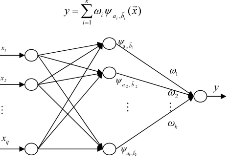
Wavelet neural networks use a three-layer structure and wavelet activation functions. The structure of a wavelet neural network with one output y, q inputs {x1,x2,…,xq} and k nodes is given in Fig. 1 [1, 5].

The output signal of this network is calculated as

∑

=

= k

i a b

i x

y

i i

1 ,

)

(r

r

ψ

ω

(1)

Fig. 1. Architecture of WNN

where xr=[x1,x2,...,x_q]T is the vector of inputs,

ω

i i = 1,2,…,k are weight coefficients between hidden

and output layers, and

i

i,b

a r

ψ

are dilated and translated versions of a mother wavelet function ℜ

→ ℜq

:

ψ

:

) ( )

( 2

,

i i q

i b

a _a

b x a x

i i

r r r

r = −

ψ

−

ψ

(2)

Naturally the mother wavelet

ψ

is required to have zero mean.

∫

ℜq

ψ

(x)dx=

∫

ℜq

ψ

(x1,x2,...,xq)dx1dx2...dxq =0

r

r ₍₃₎

and also

ψ

(xr) and

ψ

ˆ(

ω

r) rapidly decay to zero as xr →∞and

ω

r →∞.

In Eq. (2), the dilation parameter a_i∈ℜ₊ controls the support of the wavelet and the translation parameter br_i∈ℜq determines its centeral position.

In Eq. (1), if pairs (a_i,br_i) are taken from a grid

Λ

given by

{

n _m n _{n∈Z m∈Z}q

}

=

Λ (

α

, r

βα

): ,r (4) where the scalar parameters

α

and

β

define the step sizes of dilation and translation discretizations, (typically

α

=2 ,

β

=1) respectively, according to the above definitions any function f _∈L2(_ℜq) (finite-energy and continuous or discontinuous) can be approximated to an arbitrary precision by the wavelet neural network [1, 5].

The wavelets that Zhang and Benveniste [5] and Pati and Krishnaprasad [14] used in their networks are wavelet frames. Orthogonal bases are used in other wavelet networks structures [15].

1 1,b

a r

ψ

2 2,b

a r

ψ

M

1

ω

2

ω

k

ω

1 x

2 x

M

q

x

y

M

k kb a,r

In [16], a number of methods are available to construct multidimensional wavelets in both single-scaling and multi-single-scaling forms, based on one-dimensional wavelet frames. In the single-scale multidimensional wavelet frames, a single dilation parameter is used in all the dimensions of each wavelet, and multidimensional wavelet frames can be built by using a single mother wavelet. To fulfill this purpose the radial functions are used.

The single-scaling radial wavelet frames (with simpler structure than multiscaling wavelet frames) in [6] are defined as

⎭ ⎬ ⎫ ⎩

⎨ ⎧

∈ ∈ −

=

= − qn −n q

n

m x x m n Z m Z

F r (r) 2 ( r r) : , r

1

,

α

ψ

α

β

ψ

(5)

where

ψ

:ℜq →ℜ is a radial wavelet function (Like Mexican Hat wavelet) and q is the input dimension.

In the multi-scaling multidimensional wavelet frames, an independent dilation parameter is used in each dimension, and the multidimensional wavelet frames can be built by a tensor product of one dimension (1-D) wavelet functions. Using a 1-D wavelet frame

ψ

_s:ℜ→ℜ, a multi-scaling wavelet frame

ψ

:ℜq→ℜ is built by setting

( )

xr =

ψ

s

( )

x1 ...

ψ

s

( )

xq , for xr=

(

x1,...,xq

)

ψ

(6)

According to the theory of MRA, the dilation parameter of a wavelet can be interpreted as the resolution parameter. In fact, based on the multiresolution property, it is possible to present a library of wavelets. The wavelets with coarse resolution can describe the global (low frequency) behavior and those with fine resolution can describe the local (higher frequency) behavior of the approximated function. Accordingly, compared to other functional approximators, WNNs have the advantages of fast convergence, easy training and high accuracy [9].

3. FWN STRUCTURE

In the Takagi-Sugeno-Kang (TSK) model, a set of fuzzy rules can be described by

∑

=

= q

j j j i i

q q i

i

i _{IF x is A and x is A and and x is A THEN y k x}

R

1 2

2 1

1 , ... ˆ

: (7)

where i j

A is membership function, T q

x x x

xr=( 1, 2,..., ) is input vector and yˆi is output variable and a

linear combination of inputs which is essentially a global function.

In the FWN structure, yˆ_i is the output of the local model for ruleRi which is equal to the linear combination of a finite set of wavelets with the same dilation parameter.

A FWN is decribed by a set of fuzzy rules which have the following form [9]

∑

=

= i k

i i k i i

T

k

k t M t M i

i q q i

i

i _{IF x is A and x is A and and x is A THEN y x}

R

1

) (

, , 2

2 1

1 , ... ˆ ( )

: ω r ψ r r (8)

q t

M q k i

i Z t and x

M k

i

i ∈ℜ ∈ℜ

ℜ ∈

∈ ,r ,

ω

_,r r

Assuming the number of fuzzy rules is c ;1≤i≤c; T_i is the total number of wavelets for the ith rule and

i

yˆ is the output of the local model for rule Ri. t [t t, ,...,tk]

q k 2 k 1 k i =

r

5 0 , , ] ) ) / ) ((( exp[ ) ( 3 2 1 2 2 2 1 3 ≤ < ℜ ∈ − − = i j i j i j p i j i j j j i j p p p p p x x A i j (9)

In (9), pi_j1 and pi_j2 represent the center and the width of the Gaussian membership function and i

3 j

p determines the shape of the membership function.

Wavelets ( ) ( )

, x k

t M_i r

ψ

are expressed by the tensor product of 1-D wavelet functions:

∏

= − = − = q j k j j M k M k M k M k t M t x t x x i i i i i 1 ) ( 2 ) ( 2 ) ( , ) 2 ( 2 ) 2 ( 2 ) (

ψ

ψ

ψ

r r r r

(10)

According to Eq.(10), in each rule or sub-WNN, the wavelets are single-scaling and the same dilation index is in all the dimensions.

Output of the whole network is calculated as

i c

i

i x y

yˆ ˆ ( )ˆ

1

r

∑

=

=

μ

(11)

where

∑

= = _c i i i i x x x 1 ) ( ) ( ) ( ˆ r r r

μ

μ

μ

,

∏

= = q j j i j

i x A x

1 ) ( ) (r

μ

i ˆ

μ

determines the degree of contribution of each sub-WNN in the output of the network and yˆ_i is the output of the local model for rule Ri.

Notice that, in THEN-parts of fuzzy rules, FWN employs c sub-WNNs at different resolution levels to capture different behaviors (global or local) of the approximated function rather than using constants or linear equations as in the traditional fuzzy models. Unlike the traditional FNNs with only one localized approximation of function, the FWN uses both globalized and localized approximation of function. For this reason, the FWN inspired by both fuzzy model and WNN has the advantages of improved local accuracy, nicer generalization capability and faster convergence [9].

4. APPROXIMATING FEEDBACK LINEARIZATION CONTROL INPUT BY FWN

In this section, motivated by the reason stated in the previous section, we present a fuzzy wavelet network that can approximate the feedback linearization control input with high accuracy for a large group of nonlinear systems.

Consider the following qth order dynamical nonlinear system:

⎩ ⎨ ⎧ = + = ) 13 ( ) 12 ( ) ( ) ( ) ( x y u x g x f

xq r r

where f and g are unknown functions, u and y are the control input and the system output respectively, and

T q T

q x x x

x x x

x ( , ,..., ) ( , ,..., ( 1))

2 1

−

=

= &

r _{is the state vector of the system which is assumed to be available} for measurement.

Define the tracking error e as

x y y y

where yr is the desired output. According to Eqs. (12) and (13) the feedback linearization control input is

[

f x y c e

]

x g

u q T

r r r

r

r − + +

= ( )

* _{( )}

) ( 1

(15)

where cr=(c1,c2,...,c_q)T is a positive constant vector and

T q T

q ee e

e e e

e ( , ,..., ) ( , ,..., ( 1))

2 1

−

=

= &

r _{is the}

error vector.

Substituting Eq. (15) into Eq. (12), the error equation can be obtained as 0 e c ... e

c

e(q)+ q (q 1)+ + 1 =

− ₍₁₆₎

The elements in vector cr can be chosen appropriately such that all the roots of error equation are in the open left-half complex plane. Thus the controlled system is stabilized if the control input, Eq. (15), can be implemented. In practice, both f and g are unknown functions and so it is hard to implement Eq. (15). To solve the problem, a fuzzy wavelet network is proposed to approximate the feedback linearization control input.

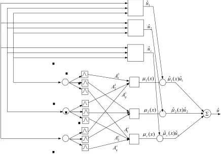
A typical fuzzy wavelet network for the approximation of (15) can be described by a set of fuzzy rules:

i

R (ith rule):

∑

=

= i k

i i k i i

T

k

k t M t M i

i q q i

i _{and x is A and and x is A THEN u x}

A is x IF

1

) (

, , 2

2 1

1 , ... ˆ

ω

r

ψ

r (r) (17)

where x_j(1≤ j≤q)is the jth state variable of xr in the controlled system (12), and uˆ_i is the control signal (output) of the local model for ith rule. The structure of fuzzy wavelet network for approximating control input (15) is given in Fig. 2 and the structure of each WNN is given in Fig. 1.

According to Eqs.(9) and (10), the output of the network in Fig. 2 is calculated as

∑

=

= c

i

i i x u

u

1

ˆ ) ( ˆ

ˆ

μ

r (18)

where

∑

=

= _c

i i i i

x x x

1

) (

) ( ) ( ˆ

r r r

μ

μ

μ

i

ˆ

μ

determines the degree of contribution of the control signal (output) of the wavelet based model with resolution level Mi .

After calculating the feedback linearization control input of FWN, the training of the network starts. Consider the training data set of the nominal model system:

{

}

≤ ≤ ∈ d ∈ℜ

l q d l d

l d

l u l L x R u

x , ) 1 ,

(r r (19) where L is the total number of the training patterns. Our goal is to train the network in Fig. 2 based on data set in (19) so that the error between the output of FWN and urd is minimized.

Most work done in the wavelet networks uses simple wavelets. For fuzzy wavelet network in [9, 10], Mexican Hat wavelet and B-spline wavelets are used respectively. We have selected the Mexican Hat

function )

2 exp( ) 1 ( ) (

2

2 x

x

x = − −

ψ

as the wavelet function and accordingly, based on data set, dilation values Mi is chosen to be in the range from -3 to 4.

input training data (desired state variables), are often redundant for constructing FWN [9]. Thus the OLS (Orthogonal Least Square) algorithm can be used for purifying wavelet candidates [6].

Σ

1

ˆ

u

2

ˆ

u

c

uˆ

) (

1 x

μ

) (

2 x

μ

)

(x

c

μ

1 1( )ˆ

ˆ x u

μ

2 2( )ˆ

ˆ xu

μ

c c(x)uˆ

ˆ

μ

uˆ

1 1

A

1 2

A

1 q

A

c

A₁

c

A₂

c q

A

Fig. 2. Structure of fuzzy wavelet network for approximating control signal

The set of wavelet candidates

{

}

w L

W =

ψ

1,

ψ

2,...,

ψ

are a set of regressor vectors which construct the

output of the network. In this step, the number of wavelet functions, S, from set W that best span the training data of the control signal are selected. Since these regressors are usually correlated, the degree of contribution of each regressor to the output energy is not clear. The OLS algorithm transforms the set of regressor vectors into a set of orthogonal basis vectors and it is possible to calculate the degree of contribution of each basis vector to the output energy [17].

From the initial set of wavelet candidates, the OLS algorithm first selects the wavelet that best fits the training data, and then repeatedly selects one of the remaining wavelets that best fits the data when combined with all previously selected wavelets. For computational efficiency, later selected wavelets are orthonormalized to earlier selected ones.

Using S selected wavelets, the approximated control signal is expressed as

( )

∑

=

= S

i

l l

s x

u

i i 1

ˆ

ω

ψ

r (20)

where {l1,l2,…,lS} is a subset of {1,2,…,Lw }. According to a set of training data as defined in (19), we can

write

u

e

( )

( )

( )

( )

(

)

(

)

(

)

T

L u u u u T L T l l l L l L l l l e e e e u u u u x x x x S S S , , , , , , , , , 2 1 2 1 1 1 2 1 1 1 L r L r L r r L

r M M

M r L r = = = ⎥ ⎥ ⎥ ⎦ ⎤ ⎢ ⎢ ⎢ ⎣ ⎡ = Ψ

ω

ω

ω

ω

ψ

ψ

ψ

ψ

u

er is the error vector of the approximation problem defined by the training data (19). Our goal is to minimize the sum of square errors

∑

= = L j uj u T

u e e

e

1 2

r

r _{. The computation of}

ω

r _{can be} performed by the least squares method. Let us define the following notations:

( )

( )

[

]

w

T L l l

i x x for i L

p

i

i 1,..., =1,2,...,

= r r

r

ψ

ψ

Then Ψis expressed as

] ,..., , [

2

1 l lS

l p p

pr r r =

Ψ (22)

Since generally the vectors

w

L 2 1,p , p

pr r …r are not mutually orthogonal, the classical or modified Gram-Schmidt algorithm can be applied to decompose Ψ as

A

Q

=

Ψ

(23) where Q=[qrl₁,qrl₂,...,qrl_S] is a

L

×

S

matrix with orthogonal columns and A is an

S

×

S

upper triangular

matrix with 1’s on the diagonal, that is

⎥ ⎥ ⎥ ⎥ ⎥ ⎥ ⎥ ⎥ ⎦ ⎤ ⎢ ⎢ ⎢ ⎢ ⎢ ⎢ ⎢ ⎢ ⎣ ⎡ = − 1 0 0 0 1 0 0 0 1 0 0 1 0 1 1 3 2 23 1 13 12 L L M O O M M L L L S S S S S A

α

α

α

α

α

α

α

Then (21) can be rewritten as

u

e v Q

ur= r+r (24) And the vector vr= A

ω

r can be determined by the least squares solution

( )

Q Q Q u

vr₌ T −1 Tr ₍₂₅₎

Since the columns of Q are orthogonal, (25) becomes

S i q q u q v v v v v i i i i S l T l T l l l l l ,..., 2 , 1 ] ,..., , [ 2 1 = = = r r r r

and the variance of ur is calculated as

∑

= + = S i u T u l T l l

T_{u v q q e e}

u _{i i i}

1

2r r r r

r

It can be seen from (26) that the term

i i

i l

T l l q q

v 2r r is the part of the variance of u explained by regressor

i l

qr . A regressor is significant if this amount is large. Therefore, error reduction ratio (err) can be defined in the following form:

u u

q q v

err _T l T l l

i i r ir i

r r

2

= (27)

The OLS method uses err to select the important wavelets which have significant contribution to the output of the network. Then Ti, i = 1, 2…c the number of selected wavelets at dilation Mi,

∑

=

=

c

1 i

i S

T the total number of selected wavelets and initial weights k

it,

M r

ω

are determined. Details of the network initialization can be found in [9].

The EKF (Extended Kalman Filter) Method is used for training parameters pi_jr , tk_j and then LS (Least-Squares) algorithm for updating k

it,

M r

ω

where j = 1,2,…,q , r = 1,2,3 , k =1,2,…,S. In [18], EKF and BP training algorithms are compared and it is shown that the EKF method has the advantages of better convergence and faster training speed.

The learning procedure will be repeated according to a performance index Ji at ith iteration which is

defined as

(

)

(

)

2

1 1

2

ˆ

∑

∑

= =

− − =

L

l d l L

l

d l l

i

u u

u u

J ,

∑

=

= L

l d l

u L u

1

1

(28)

where u_ld is the desired control input and uˆ_l is the estimated output from the FWN in Fig. 2. 5. SIMULATION RESULTS

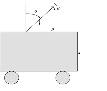
To demonstrate the capability of the proposed FWN we apply it to approximate the control signal for a second-order inverted pendulum system. In this simulation example, the objective is to approximate an appropriate control signal u to control the motion of the cart, such that the pole can track a desired output. Assume that x₁=

θ

is the angle of the pole with respect to the vertical axis, and x₂=

θ

& is the angular velocity of the pole.The inverted pendulum system is shown in Fig. 3.

The state equations can be expressed by

⎩ ⎨ ⎧

+ = =

gu f x

x x

2 2 1

& &

where

) cos 3

4 (

cos

) cos 3

4 (

cos sin sin

1 2 1

1 2

1 1 2 2 1

M m

x m L

M m

x g

M m

x m L

M m

x x mLx x

g f r

+ −

+ =

+ −

+ −

=

gr(acceleration due to gravity) = 9.81 m/s2

θ θ&

θ

Fig. 3. Inverted pendulum system

For this system our FWN has two inputs (x1, x2) and one output u. In the simulation, we use 300 pairs

{

_xrd_,ud

}

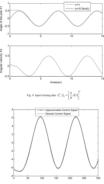
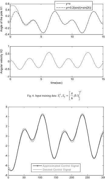
_{as training data sets of the nominal model system. By using the OLS algorithm [6], five fuzzy} rules or sub-WNN are represented to approximate the control input for tracking the desired outputy_r(t)=0.5sint (case 1). The number of the selected wavelets and dilation parameter value presented by the OLS method in each sub-WNN are given in Table 1. The total number of the selected wavelets is 17, and 74 unknown parameters are used for training.

In case 2, for tracking the desired output yr(t)=0.2(sint+sin2t), the feedback linearization control signal is approximated by 8 rules and the total number of the selected wavelets is 28. The number of the selected wavelets and dilation parameter value presented by the OLS method in each sub-WNN are given in Table 2. The performance of FWN is shown in Table 3.

Table 1. The number of the selected wavelets and dilation value in each sub-WNN for Case 1

Mi(dilation parameter value)

-4 -3 -2 -1 0 1 2

Ti (number of wavelets in each

sub-WNN) 3 2 2 2 2 4 1

Table 2. The number of the selected wavelets and dilation value in each sub-WNN for Case 2

Mi(dilation parameter value)

-4 -3 -2 -1 0 1 2 3

Ti (number of wavelets in each

sub-WNN) 5 5 2 4 3 3 3 3

Table 3. The performance of proposed FWN

yr(t) Number of _rules

Number of unknown parameters used for

training

Performance

index (Ji) Number of _iterations

Case 1 0.5sint 7 74 0.028 351

Case 2 0.2(sint+sin2t) 8 104 0.070 198

0 5 10 15 -1

-0.5 0 0.5 1

A

ngl

e of

t

he

po

le

X

1

0 5 10 15

-0.5 0 0.5 1

A

ng

ula

r v

elo

ci

ty

X

2

time(sec)

y=x yr=0.5sin(t)

Fig. 4. Input training data

T d

l x

x =_⎢⎣⎡ ,0.1_⎥⎦⎤ 6

,r₀

π

r

Fig. 5. Approximated control signal

0 50 100 150 200 250 300

-8 -6 -4 -2 0 2 4 6

8 _{Approximated Control Signal}

0 5 10 15 -0.4

-0.2 0 0.2 0.4 0.6

A

ngl

e of

t

he

po

le

X

1

0 5 10 15

-1 -0.5 0 0.5 1

A

ng

ula

r v

elo

ci

ty

X

2

time(sec) y=x

yr=0.2(sin(t)+sin(2t))

Fig. 6. Input training data

T d

l x

x = _⎢⎣⎡ ,0.1_⎥⎦⎤ 6

, 0

π

r r

Fig. 7. Approximated control signal

0 50 100 150 200 250 300

-8 -6 -4 -2 0 2 4 6

6. CONCLUSIONS

In this paper, we presented a fuzzy wavelet network for approximating feedback linearization control input in which the mathematical model of the controlled system is unknown. The proposed FWN with the combination of WNN and fuzzy logic has advantages of the approximation accuracy and good generalization performance. Fuzzy rules correspond to sub-WNNs with different resolution levels such that the degree of contribution of various sub-WNNs can be controlled flexibly. The obtained results of simulation examples demonstrated the efficiency of the presented approach.

REFERENCES

1. Iyengar, S. S., Cho, E. C. & Phoha, V. V. (2002). Foundations of waveletnetworks and applications. CRC Press.

2. Billings, S. A. & Wei, H. L. (2005). A new class of wavelet networks for nonlinear system identification. IEEE Trans. Neural Net. Vol. 16, pp. 826-874.

3. Lin, F. J., Shieh, H. J. & Huang, P. K. (2006). Adaptive wavelet neural network control with hysteresis estimation for piezo-positioning mechanism. IEEE Trans, Neural Net., Vol. 17, No. 2, pp. 432-444.

4. Chui, C. K. (1992). An introduction to wavelets. Academic Press, NY, U.S.A.

5. Zhang, Q. & Benveniste, A. (1992). Wavelet networks. IEEE Trans. Neural Net., Vol. 3, No. 6, pp. 889-898. 6. Zhang, Q. (1997). Using wavelet network in non Parametric estimation. IEEE Trans. Neural Networks, Vol. 8,

No. 2, pp. 227-236.

7. Jane, J. S. R., Sun, C. T. & Mizutani, E. (1997). Neuro-fuzzy and soft computing. Engle Wood Cliffs, NJ: Prentice-Hall.

8. Tahani, V. & Sheikholeslam, F. (1999). Total stability of fuzzy feedback control systems. Iranian Journal of Science & Technology, Vol. 23, No. 1, pp. 27-34.

9. Ho, D. W. C., Zhang, P. A. & Xu, J. (2001). Fuzzy wavelet networks for function learning. IEEE Trans. Fuzzy Systems, Vol. 9, No. 1, pp. 200-211.

10. Wang, J., Xiao, J. & Hu, D. (2005). Fuzzy wavelet network modelling with B-spline wavelet. Proceedings of International Conference on Machine Learning and Cybernetics, Vol. 7, pp. 4144-4148.

11. Abiyev, R. H. (2005). Controller based of fuzzy wavelet neural network for control of technological processes.

IEEE International Conference on CIMSA, pp. 215-219.

12. Slotin, J. E. & Li, W. (1991). Applied nonlinear control. Englewood Cliffs, NJ: Prentice Hall International. 13. Khalil, H. K. (2005). Nonlinear systems. Third Edition, Prentice Hall.

14. Pati, Y. & Krishnaprased, P. (1993). Analysis and synthesis of feedforward neural networks using discrete affine wavelet transformation. IEEE Trans. Neural works, Vol. 4, No. 1, pp. 73-85.

15. Zhang, J., Walter, G. G. & Lee, W. N. W. (1995). Wavelet neural networks for function learning. IEEE Trans. Signal Processing, Vol. 43, No. 6, pp. 1485-1497.

16. Kugarajah, Th. & Zhang, Q. (1995). Multidimensional wavelet frames. IEEE Trans. Neural Networks, Vol. 6, No. 6, pp. 1552-1556.

17. Chen, S., Cowan, C. F. N. & Grant, P. M. (1991). Orthogonal least squares learning algorithm for radial basis function networks. IEEE Trans. Neural Networks, Vol. 2, No. 2, 302-309.