MONETARY POLICY AND FINANCIAL
CONDITIONS IN INDONESIA
Solikin M. Juhro1, Bernard Njindan Iyke2
1 Bank Indonesia Institute, Bank Indonesia, Jakarta, Indonesia. Email: solikin@bi.go.id
2 Centre for Financial Econometrics, Deakin Business School, Deakin University,
Melbourne, Australia. Email: bernard@deakin.edu.au
We develop a financial condition index (FCI) and examine the effects of monetary policy on financial conditions in Indonesia. We show that our FCI tracks financial conditions quite well because it captures key financial events (the Asian financial crisis of 1997–1998, the Indonesian banking crisis, and the global financial crisis and its aftermath). A unique feature of our FCI is that it is quarterly and thus offers near real-time development in financial conditions. We also show that monetary policy shapes the FCI. A contractionary monetary policy leads to unfavourable financial conditions during the first two quarters, followed by favourable financial conditions for nearly three quarters. This finding is robust to an alternative identification strategy. Our findings highlight the critical role of the monetary authority in shaping financial conditions in Indonesia.
Article history:
Received : September 15, 2018 Revised : January 2, 2019 Accepted : January 4, 2019 Available online : January 30, 2019 https://doi.org/10.21098/bemp.v21i3.1005
Keywords: Financial conditions; Monetary policy; Indonesia. JEL Classifications: E44; E52.
3 The other two are South Korea, and Thailand. I. INTRODUCTION
We create a new financial condition index (FCI) and analyse the effect of monetary policy on financial conditions in Indonesia. An FCI is a single indicator constructed to capture facets of the financial sector. Changing financial conditions are important for both policymakers and investors (Koop and Korobilis, 2014). Thus, a unique index to capture changing financial conditions has become popular in recent times. The debate on FCIs centres around what econometric approach and indicators of financial conditions should be used when constructing FCIs. For instance, Freedman (1994) contends that an FCI should capture exchange rate movements, whereas Dudley and Hatzius (2000) recommend the need for large-scale macroeconomic indicators. In terms of approaches, two are mainly identified in the literature. The first, the so-called weighted-sum approach, involves assigning weights to the various indicators of financial conditions (Debuque-Gonzales and Gochoco-Bautista, 2017). The weighting scheme derives from the relative impact on the real gross domestic product of each indicator, by simulating either structural or reduced-form macroeconomic models. The second approach is based on extracting common factors from a set of financial indicators using factor analysis or principal components analysis (Brave and Butters, 2011; Koop and Korobilis, 2014).
Among the earliest studies to construct FCIs are those of Goodhart and Hofmann (2001) and Mayes and Virén (2001), who note that house and stock prices are important drivers of financial conditions in the United Kingdom and Finland. Others, including Gauthier, Graham, and Liu (2004), Guichard and Turner (2008), and Swiston (2008), find corporate bond yield risk premiums and credit availability to be critical when constructing FCIs for Canada and the United States. FCIs have been extended to other economies, notably the Asian economies. Admittedly, the FCI literature in the Asian context is sparse. Studies such as those of Guichard, Haugh, and Turner (2009) and Shinkai and Kohsaka (2010) emphasize credit market conditions when constructing an FCI for Japan, while that of Osorio, Unsal, and Pongsaparn (2011) combine common factor and weighted-sum approaches when constructing FCIs for Asian economies. Debuque-Gonzales and Gochoco-Bautista (2017) have recently constructed FCIs for Asian economies using factor analysis.
the peak of the AFC (Iyke, 2018a). Agung, Juhro, and Harmanta (2016) argue that monetary policy alone is not sufficient to maintain macroeconomic stability and recommend complementary policies in Indonesia. In this regard, it is evident that understanding the evolution of the country’s financial conditions will go a long way in helping policymakers pre-empt future deterioration and enhance stability.
Second, the impact of monetary policy on financial conditions in Indonesia and other Asian economies is poorly understood. Debuque-Gonzales and Gochoco-Bautista (2017) examine this issue but use annual data. Policymakers and investors alike are arguably more interested in the reactions of markets at higher frequencies to policy surprises as evidenced in their decisions. For instance, monetary policy decisions are carried out on a quarterly basis. Similarly, firms announce their financial reports quarterly. Thus, a great deal of information is lost when annual data are used. We circumvent this problem by employing quarterly data. In addition, we deal with the well-known price and exchange rate puzzles when identifying monetary policy shocks by including commodity prices and using an alternative recursive ordering of the variables in the model.4
The main goal of monetary policy is to achieve macroeconomic and price (or monetary) stability. As argued by Juhro and Goeltom (2013), macroeconomic and price stability are tied to financial system stability in Indonesia because they are interlinked. Therefore, since financial conditions generally shape the direction of the economy (i.e. they serve as a leading indicator of business activities), our FCI would be a useful tool to enhance the decisions of participants in the Indonesian economy. We find that our FCI tracks financial conditions quite well. For instance, it captures the peaks of the AFC and the Indonesian banking crisis, the relatively stable period from 2000 until 2008, and the global financial crisis and its aftermath. This is consistent with previous FCIs. A unique feature of our FCI is that it is quarterly and thus offers near real-time development in financial conditions. We also find that monetary policy shapes the FCI. A contractionary monetary policy leads to unfavourable financial conditions within the first two quarters. Financial conditions then improve for nearly three quarters, before declining. This finding is robust to an alternative identification strategy. Our findings highlight the critical role of the monetary authority in shaping financial conditions in Indonesia.
The remainder of the paper is organized as follows. Section II presents the model specification and the data. Section III discusses the results. Section IV concludes the paper.
II. MODEL SPECIFICATION AND DATA
A. Model Specification
This section outlines the approach used to construct the FCI. It also presents a Vector Autoregressive (VAR) model to examine the effect of monetary policy on financial conditions.
4 The price puzzle is a phenomenon whereby general prices react to a contractionary monetary policy
5 In application, maximum likelihood is implemented in two steps. In the first step, the model is
presented in state-space form. In the second step, the Kalman filter is used to derive and solve the log likelihood equation (Stock and Watson, 1991).
A1. Dynamic Factor Model to Construct the FCI
We construct the FCI by employing a dynamic factor model. Given a set of endogenous variables (e.g. various indicators of economic and financial conditions), the dynamic factor model assumes that these variables are linear functions of certain unobserved factors and exogenous variables. The unobserved factors are therefore said to capture the movements of the set of endogenous variables. In theory, the unobserved factors and disturbances in the model are assumed to follow known correlation structures (Geweke, 1977; Stock and Watson, 1991). Following the literature (e.g. Geweke, 1977; Sargent and Sims, 1977), the following dynamic factor model can be specified:
where y is a vector of dependent variables, f is a vector of unobservable factors, x and w are vectors of exogenous variables, u, v, and ϵ are vectors of disturbances, P, Q, and R are matrices of parameters, A and C are matrices of autocorrelation parameters, and t, p, and q are time and lag subscripts, respectively.
In our application, y contains the indicators of financial conditions (exchange rate, credit, interest rates, equity indices, and business conditions). These indicators are modelled as linear functions of unobserved factors assumed to follow a second-order autoregressive process, to capture persistence in financial conditions. The FCI is the predicted vector of unobservable factors f (a one-step-ahead forecast of ̂ f). Following Stock and Watson (1991), we estimate the dynamic factor model by maximum likelihood.5
A2. VAR Model for the Indonesian Economy
We link monetary policy to financial conditions by estimating the following VAR model for the Indonesian economy:
(1) (2) (3)
, (4)
6 See, for example, Bernanke (1986), Blanchard and Watson (1986), Blanchard and Quah (1989), Uhlig (2005), and Rubio-Ramírez, Waggoner, and Zha (2010). Each approach has its advantages and
disadvantages.
7 Note that, since 2005 (under the inflation targeting framework), Bank Indonesia has used different
policy rates. From 2005 until mid-2016, the bank used the Bank Indonesia Certificate (Sertifikat Bank
Indonesia). Then, since mid-2016, the bank has used a seven-day reverse repo rate. These rates are slightly different (i.e. the former is around 150 basis points higher than the latter). This does not imply that Bank Indonesia has pursued an expansionary monetary policy, since the two rates have
the same term structure. There has been no change in policy stance.
The policy shock is identified through the one-step-ahead forecast error, ut. Such a shock is structural and is transmitted to the entire economy. In practice, however, the decomposition of ut and an economically meaningful explanation of the structural shocks have remained a controversial topic. If we normalize ut into vt such that E[vt vt’ ]=I
n, then there exists a matrix A such that ut=Avt. The jth
column of A denotes the instantaneous impact of the jth fundamental innovation
on all the variables. This fundamental innovation has one standard error in size (Uhlig, 2005; Iyke, 2018b). Therefore, A is restricted by the variance–covariance matrix as follows:
Equation (5) indicates n(n-1)/2 degrees of freedom remaining in the model, which is not sufficient when identifying shocks to ut. There are several approaches to address this problem.6 Consistent with Sims (1986), we do so by restricting A to be a Cholesky factor of Σ. In other words, we use a recursive ordering of Yt when identifying shocks to ut.
B. Data
Our sample covers the period 1994: Q1 to 2018: Q4. To construct the FCI, we use various variables indicating specific aspects of the financial conditions in Indonesia. We use Bank Indonesia’s rate (IRATE)7 for the interest rate channel, the nominal effective exchange rate (NER) for the exchange rate channel, banking system claims on private enterprise (CREDIT) for the credit channel, the Jakarta Composite Index (JCI) and the MSCI Share Price Index (MSCI) for the equity channel, and the business confidence index (BCI) and the consumer confidence index (CCI) for the expectation or perception channel. In the VAR model, we use the manufacturing production index (MP), the growth in CPI, the FCI, the commodity price index (COM), NER, the short-term interest rate or monetary policy rate (STR), and the monetary base or money supply (M2). The movements of these variables are shown in Figure A1 in the Appendix and the summary statistics and further details on the variables are presented in Tables A1 and A2, respectively.
III. RESULTS
A. Measuring Financial Conditions
We begin our analysis by testing for unit roots in the indicators of financial conditions. These results are shown in Table 1. There is no strong evidence to reject the unit root null hypothesis. Therefore, we proceed to constructing the FCI by modelling the indicators in their first differences as linear functions of an unobserved factor. The unobserved factor is assumed to follow a second-order autoregressive process.
This table reports unit root test results based on the Augmented Dickey-Fuller (ADF) and the Perron and Vogelsang (PV, 1992)
breakpoint tests. The null hypothesis is that there is a unit root. The breakpoint type is an innovation outlier. The break point is
selected by minimizing the Dickey-Fuller statistic. A maximum of 12 lags is included in these models. Finally, ** and *** denote, respectively, 5% and 1% significance levels.
Variable
ADF test PV test
Zt-statistic (Lag) Innovation outlier Constant Constant and Trend t-statistic (Lag) Break date
IRATE -1.706(1) -2.324(1) -3.614(3) 2008M10
lnBCI -2.656(0)* -4.316(0)*** -4.305(0)* 2009M01
CCI -3.876(4)*** -4.469(4)*** -7.621(0)*** 2002M02
lnCREDIT -1.711(2) -0.997(2) -4.140(0) 2000M08
lnNER -2.112(2) -2.510(1) -5.546(2)*** 1997M07
lnJCI -0.398(1) -2.660(1) -3.030(2) 2003M03
lnMSCI -2.210(0) -1.734(0) -3.938(0) 1998M07
Table 1.
Tests for Unit Roots in FCI Constituents
Table 2 shows the maximum likelihood estimates of the dynamic factor model. Because two of the constituents of the FCI, the business confidence index (BCI) and the consumer confidence index (CCI) have a short time span (i.e. they start in 2000:Q1, whereas the others start in 1994:Q1), we estimate the dynamic factor model with and without these variables. The seven variables used for the dynamic factor model are IRATE, NER, CREDIT, JCI, MSCI, BCI, and CCI. Model (1) contains all seven variables, whereas model (2) contains all seven except
for BCI and CCI. Both models generally indicate some degree of persistence in
Figure 1 shows the extracted FCI values plotted against changes in interest rates and Figure 2 shows only the FCIs.8 The period between 1997 and 2002 was turbulent. Financial conditions worsened between 1997 and 1998, which were the peaks of the AFC and the Indonesian banking crisis (Iyke, 2018a). This time is followed by enhanced financial conditions between 1998 and 1999, a sharp decline between 1999 and 2001, and subsequent improvement between 2001 and 2002. Beyond this deterioration and recovery phase, financial conditions were moderate and stable in the country until a marked decline and subsequent recovery between 2008 and 2010. The fluctuations in our FCI look a bit similar to those of the annual FCI developed by Debuque-Gonzales and Gochoco-Bautista (2017). Of course, ours edges out theirs, in that it is quarterly and thus offers near real-time development in financial conditions. Policymakers and analysts alike are more concerned with developments in financial conditions at higher frequencies, as reflected in monetary policy announcements and quarterly financial reports. The next section therefore analyses how movements in our FCI are shaped by monetary policy.
This table reports estimates of the dynamic factor model. The constituents of the FCI are specified in their first-differences as linear functions of an unobserved factor. The unobserved factor (i.e. the FCI) is assumed to follow a second-order autoregressive process.
Models (1) and (2) contain, respectively, estimates with and without lnBCI and CCI. The full sample period is from 1994: Q1 to 2018:
Q4. Finally, * (**) *** denote statistical significance at the 10% (5%) 1% levels.
Variables Coefficient (z-statistic)
Factor Model (1) Model (2)
Lag 1 0.432***[3.650] 0.507**[2.230]
Lag 2 -0.171[-1.440] -0.027 [-0.260]
∆IRATE -0.238***[-3.000] -0.063***[-3.400]
∆lnNER 0.014***[3.490] 0.005[1.590]
∆lnCREDIT 0.010[0.290] -0.004[-0.310]
∆lnJCI 0.108***[11.750] 0.018***[4.740]
∆lnMSCI 0.021*[1.820] -0.002[-0.600]
∆lnBCI 0.017**[2.090]
∆CCI 1.964*[1.820]
Log likelihood -13.884 1503.705
Wald Chi-square (8) 152.100 410.560
Prob > Chi-square 0.000 0.000
Number of observations 69 296
Sample 2001Q2 – 2018Q4 1994Q1 – 2018Q4
Table 2.
Dynamic Factor Estimates
8 The FCI with BCI and CCI appears to be smaller in absolute terms than the FCI without these two variables. The former captures the key FCI determinants and is therefore a more accurate indicator
Figure 1. FCI Movement
This graph shows the movements of the FCI (with and without BCI and CCI) and interest rates (1994: Q1 to 2018: Q4).
-20 -10 0 10 20 30
1995q1 2000q1 2005q1 2010q1 2015q1 2020q1
Interest rate growth
FCI with BCI and CCI FCI without BCI and CCI
Figure 2. FCI for Indonesia
This graph shows the movements of the FCI for Indonesia (1994: Q1 to 2018: Q4).
-10 -5 0 5 10
1995q1 2000q1 2005q1 2010q1 2015q1 2020q1
FCI with BCI and CCI FCI without BCI and CCI
B. Impact of Monetary Policy on Financial Conditions
not properly safeguarded, can implode, owing to excessive speculative activities and lack of due diligence, especially in the area of credit allocation. The recent global financial crisis was mainly triggered by these factors.
In this section, we explore how financial conditions respond to monetary policy shocks (or surprises). In other words, we analyse how financial conditions respond to a sudden monetary policy contraction or expansion. We identify a monetary policy shock as an innovation in the short-term policy rate (STR). The monetary policy shock is based on a Cholesky decomposition of the variance– covariance matrix in equation (5), whereby STR is ordered last. We overcome the price and exchange rate puzzles by including the nominal exchange rate and commodity prices. The commodity prices are exogenous; therefore, lnCOM
is ordered behind the monetary policy variable, STR. In terms of the degree of
exogeneity of the remaining variables, we assume that FCI is the most endogenous variable and we therefore order it first, followed by lnCPI (indicating demand push inflation pressures) and output (lnMP), in that order. Specifically, our benchmark identification equation is
In addition to imposing lower triangularity on A in equation (5), we impose on (B,Σ) a flat normal inverted-Wishart prior.9 We generate impulse response functions (IRFs) via 1,000 Markov chain Monte Carlo draws, a horizon of 10 quarters ahead, and two lags.10 The shock is one standard deviation in size. Thus, IRFs are bounded by the 16th and the 84th percentiles.
The resulting graph is shown in Figure 3. A contractionary monetary policy shock leads to unfavourable financial conditions (a decline in FCI below zero) one quarter after the shock. This deterioration in financial conditions persists until the end of the second quarter. Financial conditions improve (FCI rises above zero) for nearly three quarters before declining. We track the robustness of the FCI response to contractionary monetary policy by obtaining IRFs from an alternative ordering strategy. In this case, STR is ordered second but last. This identification is motivated by previous studies (e.g., Christiano, Eichenbaum, and Evans, 1999; Uhlig, 2005), which argue that monetary policy has an immediate effect only on the policy rate (short-term rate). Because monetary policy has a delayed effect on the economy (Christiano, Eichenbaum, and Evans, 1999), we order FCI first. Stated formally, our ordering strategy is
(6)
9 Canova (2007) provides technical details on this prior restriction.
10 We impose two lags because of considerations of sample size and degree of freedom.
note that such a relationship tends to reverse the impact of expansionary monetary policy. We document that expansionary monetary policy is linked with favourable financial conditions for the first few quarters. In the medium term, our findings appear to corroborate theirs, in that financial conditions appear to decline, perhaps due to the reduction in risk-taking activities and credit facilities.
Figure 3. Response of FCI to Monetary Policy Shocks
This figure shows the response of financial conditions to a contractionary monetary policy shock of one standard deviation in size, which is identified as the innovation in the short-term interest rate, ordered last in Cholesky decomposition. The FCI is ordered
first, followed by lnCPI. The three lines denote the 16% quantile, the median and the 84% quantile of the posterior distribution.
-0,8 -0,4 0,0 0,4 0,8 1,2
1 2 3 4 5 6 7 8 9 10
Response to Cholesky One S.D. Innovations ± 2 S.E.
Figure 4. Response of FCI to Monetary Policy Shocks – Alternative Ordering This figure shows the response of financial conditions to a contractionary monetary policy shock of one standard deviation in size, which is identified as the innovation in the short-term interest rate, ordered last in the Cholesky decomposition. The FCI is placed
first, followed by lnMP. The three lines denote the 16% quantile, the median and the 84% quantile of the posterior distribution.
-,4 -,2 ,0 ,2 ,4 ,6 ,8
1 2 3 4 5 6 7 8 9 10
IV. CONCLUSION
We create a new FCI and analyse the effect of monetary policy on financial conditions in Indonesia. There are, so far, only limited FCI studies on Asian economies. These studies are based on a panel of Asian economies; however, these countries are interlinked through trade and, therefore, analysis of the unique attributes of their FCIs becomes highly tasking within a single framework. We address this issue by solely focusing on Indonesia.
Indonesia has undergone substantial changes in terms of financial conditions, making it appealing for this study. The country is among the three that were most affected by the AFC. It has also, in recent times, experienced the sharpest depreciation in its currency since the peak of the AFC. Good FCIs would enhance authorities’ abilities to pre-empt future deterioration in financial conditions. In addition, there is little understanding of the impact of monetary policy on financial conditions in Indonesia and other Asian economies. Previous attempts have used annual data, which might not be appealing, because policymakers and investors are arguably more interested in the reactions of markets to policy surprises at higher frequencies, as evidenced in their decisions. We address this point by employing quarterly data.
We find that our FCI tracks financial conditions quite well. For instance, it captures the peaks of the AFC and the Indonesian banking crisis, the relatively stable period from 2000 until 2008, and the global financial crisis and its aftermath. This is consistent with previous FCIs. A unique feature of our FCI is that it is quarterly and thus offers near real-time development in financial conditions. We also find that monetary policy shapes the FCI. A contractionary monetary policy leads to unfavourable financial conditions between the first and second quarters. Financial conditions then improve for nearly three quarters, before declining. This finding is robust to an alternative identification strategy. Our findings highlight the critical role of the monetary authority in shaping financial conditions in Indonesia. In this case, a significant countercyclical monetary policy impact on financial conditions opens up room to augment the standard monetary policy rule by incorporating an unexpected development (deviation) of financial conditions.
REFERENCES
Agung, J., Juhro, S. M., & Harmanta, T. (2016) Managing Monetary and Financial Stability in a Dynamic Global Environment: Bank Indonesia’s Policy Perspectives (October 2016). BIS Paper No. 88f. Available at SSRN: https://ssrn. com/abstract=2861312.
Bernanke, B. S. (1986). Alternative Explanations of the Money–Income Correlation. In: Brunner, K., & Meltzer, A. (Eds.), Real Business Cycles, Real Exchange Rates, and Actual Policies. Carnegie-Rochester Conference Series on Public Policy, vol. 25. North-Holland, Amsterdam.
Blanchard, O., & Watson, M. (1986). Are All Business Cycles Alike? In: Gordon, R.J. (Ed.), The American Business Cycle. University of Chicago Press, Chicago, 123–160.
Blanchard, O. J., & Quah, D. (1989). The Dynamic Effects of Aggregate Demand
Brave, S., & Butters, R. (2011). Monitoring Financial Stability: A Financial Conditions Index Approach. Economic Perspectives, 35, 22–43.
Canova, F. (2007). Methods for Applied Macroeconomic Research. Princeton, NJ: Princeton University Press.
Christiano, L., Eichenbaum, M., & Evans, C. (1999). Monetary Policy Shocks: What Have I Learned and to What End? In: Woodford, M., Taylor, J.B. (Eds.),
Handbook of Macroeconomics. North-Holland, Amsterdam, 65–148.
Cushman, D. O., & Zha, T. (1997). Identifying Monetary Policy in a Small Open Economy Under Flexible Exchange Rates. Journal of Monetary Economics, 39, 433-448.
Debuque-Gonzales, M., & Gochoco-Bautista, M. S. (2017). Financial Conditions Indexes and Monetary Policy in Asia. Asian Economic Papers, 16, 83-117. Dudley, W., & Hatzius, J. (2000). The Goldman Sachs Financial Conditions Index:
The Right Tool for a New Monetary Policy Regime. Global Economics Paper No. 44.
Freedman, C. (1994). The Use of Indicators and of the Monetary Conditions Index in Canada. Frameworks for monetary stability: policy issues and country experiences, 458-476.
Gauthier, C., Graham, C., & Liu, Y. (2004). Financial Conditions Indexes for
Canada. Bank of Canada Working Paper No. 2004–22.
Geweke, J. (1977). The Dynamic Factor Analysis of Economic Time Series Models. In Latent Variables in Socioeconomic Models, ed. D. J. Aigner & A. S. Goldberger, 365–383. Amsterdam: North-Holland.
Goldstein, M. (1998). The Asian Financial Crisis: Causes, Cures, and Systemic Implications. Peterson Institute, 55.
Goodhart, C., & Hofmann, B. (2001). Asset Prices, Financial Conditions, and The Transmission of Monetary Policy. In conference on Asset Prices, Exchange Rates, and Monetary Policy (March, 2001), Stanford University (2-3).
Guichard, S., & Turner, D. (2008). Quantifying the Effect of Financial Conditions
on US Activity. OECD Economics Department Working Paper No. 635.
Guichard, S., Haugh, D., & Turner, D. (2009). Quantifying the Effect of Financial Conditions in the Euro Area, Japan, United Kingdom, and United States.
OECD Economics Department Working Paper No. 677.
Iyke, B.N. (2018a) A Test of the Foreign Exchange Market Efficiency in Indonesia.
Bulletin of Monetary Economics and Banking (forthcoming).
Iyke, B. N. (2018b). Assessing the Effects of Housing Market Shocks on Output: The Case of South Africa. Studies in Economics and Finance, 35, 287-306.
Juhro, S. M., & Goeltom, M. (2013) The Monetary Policy Regime in Indonesia (November 1, 2013). Macro-Financial Linkages in Pacific Region, Akira Kohsaka (Ed.), Routledge, February 2015. Available at SSRN: https://ssrn.com/ abstract=2875631.
Koop, G., & Korobilis, D. (2014). A New Index of Financial Conditions. European Economic Review, 71, 101-116.
Rubio-Ramírez, J., Waggoner, D., & Zha, T. (2010). Structural Vector Autoregressions: Theory of Identification and Algorithms for Inference. Review of Economic Studies, 77, 665-696.
Satria, D., & Juhro, S. M. (2011). Risk Behavior in the Transmission Mechanism of
Monetary Policy in Indonesia. Bulletin of Monetary Economics and Banking, 13,
243-270.
Sargent, T. J., & Sims,C. A. (1977). Business Cycle Modeling without Pretending to Have too much a Priori Economic Theory. In New Methods in Business Cycle Research: Proceedings from a Conference, ed. C. A. Sims, 45–109. Minneapolis: Federal Reserve Bank of Minneapolis.
Shinkai, J.-I., & Kohsaka, A. (2010). Financial Linkages and Business Cycles of Japan: An Analysis Using Financial Conditions Index. OSIPP Discussion Paper
No. 2010-E-008. Osaka School of International Public Policy.
Sims, C. A. (1986). Are Forecasting Models Usable for Policy Analysis. Minneapolis Federal Reserve Bank Quarterly Review Winter, 2–16.
Sims, C. A. (1992). Interpreting the Macroeconomic Time Series Facts. European Economic Review, 36, 975–1011.
Stock, J. H., & Watson, M. W. (1991). A Probability Model of the Coincident
Economic Indicators. In Leading Economic Indicators: New Approaches and
Forecasting Records, ed. K. Lahiri and G. H. Moore, 63–89. Cambridge: Cambridge University Press.
Swiston, A. (2008). A U.S. Financial Conditions Index: Putting Credit where Credit is Due. IMF Working Paper No. 08/161.
Osorio, M. C., Unsal, D. F., & Pongsaparn, M. R. (2011). A Quantitative Assessment of Financial Conditions in Asia (No. 11-170). International Monetary Fund. Perron, P., & Vogelsang, T. J. (1992). Nonstationarity and Level Shifts with an
Application to Purchasing Power Parity. Journal of Business & Economic Statistics, 10, 301-320.
Uhlig, H. (2005). What are the Effects of Monetary Policy on Output? Results from an Agnostic Identification Procedure. Journal of Monetary Economics, 52, 381-419.
APPENDIX
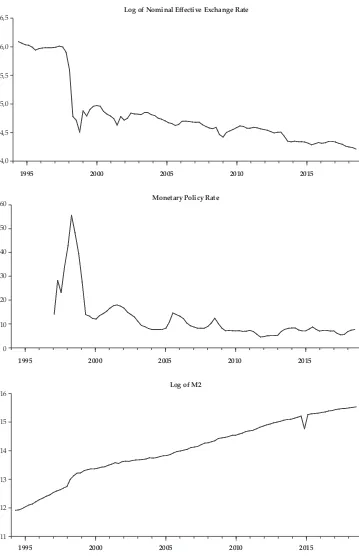
Figure A1. Variables Used for Constructing FCI and the VAR Model
This figure shows the behaviour of the variables used in constructing the FCI and the VAR model. The first seven graphs are the
financial condition indicators used in the FCI model. The last seven (including lnNER) graphs are those variables used in the VAR
model to examine the impact of monetary policy shocks on financial conditions. The maximum sample period employed is from 1994: Q1 to 2018: Q4.
0 20 40 60 80
1995 2000 2005 2010 2015
Interest Rate
4,0 4,2 4,4 4,6 4,8 5,0
1995 2000 2005 2010 2015
Figure A1. Variables Used for Constructing FCI and the VAR Model (Continued)
-20 -10 0 10 20 30
1995 2000 2005 2010 2015
Consumer Confidence Index
5 6 7 8 9
1995 2000 2005 2010 2015
Log of Jakarta Composite Index
4,0 4,5 5,0 5,5 6,0 6,5
1995 2000 2005 2010 2015
Figure A1. Variables Used for Constructing FCI and the VAR Model (Continued)
4 6 8 10 12
1995 2000 2005 2010 2015
Log of Credit to Private Sector
5 6 7 8 9
1995 2000 2005 2010 2015
Log of MSCI Index
-8 -4 0 4 8 12
1995 2000 2005 2010 2015
Figure A1. Variables Used for Constructing FCI and the VAR Model (Continued)
3,8 4,0 4,2 4,4 4,6 4,8
1995 2000 2005 2010 2015
Log of Manufacturing Production Index
2,5 3,0 3,5 4,0 4,5 5,0
1995 2000 2005 2010 2015
Log of CPI
6,5 7,0 7,5 8,0 8,5 9,0
1995 2000 2005 2010 2015
Figure A1. Variables Used for Constructing FCI and the VAR Model (Continued)
4,0 4,5 5,0 5,5 6,0 6,5
1995 2000 2005 2010 2015
Log of Nominal Effective Exchange Rate
0 10 20 30 40 50 60
1995 2000 2005 2010 2015
Monetary Policy Rate
11 12 13 14 15 16
1995 2000 2005 2010 2015
Table
A1.
Summary Statistics of the V
ariables This table shows the summary statistics of the variables used in constructing the FCI and the VAR model. The first sev en variables are the financial condition indicators used in the FCI model. The last six variables (including ln NER ) are those used in the VAR model to examine the impact of monetary policy shocks on financial conditions. Details on these variables are shown in Table A2 below. The maximum
sample period employ
ed is from 1994: Q1 to 2018: Q4. IRA
TE lnBCI CCI lnJCI lnNER lnCREDIT lnMSCI FCI lnMP lnCPI lnCOM MPR lnM2 Mean 11.4595 4.6168 9.3669 7.2689 4.8170 8.4910 7.9132 -0.0228 4.3013 3.8927 7.7550 11.8368 14.0364 Median 8.2500 4.6697 11.2094 7.1833 4.6568 8.9695 8.4273 -0.0292 4.2633 4.0636 7.8521 8.1088 14.0408 Maximum 63.9867 4.8296 21.9900 8.774 6.0981 10.5924 8.9346 8.9801 4.7152 4.7121 8.6577 55.9093 15.5501 Minimum 4.2500 4.1395 -11.7400 5.8908 4.2186 5.0304 5.9829 -6.8701 3.9158 2.5649 6.7893 4.3788 11.9129 Std. Dev. 9.4723 0.1653 7.8302 1.0123 0.5439 1.8596 0.9587 1.8880 0.2021 0.6530 0.6207 9.4480 1.0258 Skewness 3.5915 -0.8707 -0.7191 0.0939 1.4211 -0.7943 -0.7542 1.1774 0.3713 -0.6607 -0.1499 2.8066 -0.3591 Kurtosis 17.5034 2.9748 2.9952 1.3643 3.7314 2.2045 2.0083 12.5296 2.2989 2.2684 1.4112 11.2036 2.2016 Jarque-Bera 1091.4360 8.9732 6.5492 11.2948 35.8855 13.0210 13.5779 397.4757 4.2152 9.4113 10.7835 358.1764 4.8051 Probability 0.0000 0.0113 0.0378 0.0035 0.0000 0.0015 0.0011 0.0000 0.1215 0.0090 0.0046 0.0000 0.0905 Sum 1145.945 327.7949 711.8835 726.8904 481.6957 840.6125 791.3154 -2.2614 417.2214 385.3742 767.7429 1029.8010 1403.639
Sum Sq. Dev.
Table
A2.
Details on the V
ariables This table shows details on the variables used in constructing the FCI and the VAR model. The first sev en variables are the financial indicators used in the FCI model. The last six variables (including ln NER )
are those used in the V
AR model to examine the impact of monetary policy shocks on fina
ncial conditions. The maximum sample period employ
ed is from 1994: Q1 to 2018: Q4.
Indicator Variable Period Source IRA TE Interest rate proxied by the Bank Indonesia (BI) rate (From July 2005 to July 2016, w e use ‘implicit rate’ anchoring to 1-month BI certificate rate; since July 2016, w e use 7-D rev erse repo rate (money market); a new policy rate does not change the stance of BI monetary policy as old rate and new rate are in the same term
structure (different tenors)
1994Q1 – 2018Q4
Bloomberg
lnBCI
Logarithm of the business confidence index (Business
Activity Surv
ey)
2000Q1 – 2018Q4
Statistics Indonesia
CCI
Consumer confidence index
2001Q2 – 2018Q4
Statistics Indonesia
lnJCI
Logarithm of the Jakarta Composite Price Index
1994Q1 – 2018Q4
Bloomberg
lnNER
Logarithm of the nominal effectiv
e exchange rate
1994Q1 – 2018Q4
Bloomberg
lnCREDIT
Logarithm of the banking system: claims on priv
ate sector
1994Q1 – 2018Q3
Bloomberg
lnMSCI
Logarithm of the MSCI Share Price Index
1994Q1 – 2018Q4
Bloomberg
FCI
Financial condition index computed as using dynamic factor of a
bov
e v
ariables
1994Q1 – 2018Q3
Computed
lnMP
Logarithm of the total manufacturing production for Indonesia (
2015 =100)
1994Q1 – 2018Q1
Federal Reserv
e
Bank of St. Louis
lnCPI
Logarithm of the consumer price index
1994Q1 – 2018Q3
Federal Reserv
e
Bank of St. Louis
lnCOM Logarithm of the commodity price index computed as PCA of crude oil, natural gas Index (2010=100),
copper, and gold
1994Q1 – 2018Q3
Word Bank
MPR
Monetary policy rate proxied by 91-day Treasury Bill rate (BI i
nterbank offering rate 3-month)
1997Q2 – 2018Q4
Bloomberg
lnM2
Logarithm of money supply (M2)
1994Q1 – 2018Q4