Classifying heartrate by change detection and wavelet methods for emergency physicians*

J.-S. Dhersin, Editor

CLASSIFYING HEARTRATE BY CHANGE DETECTION AND WAVELET

METHODS FOR EMERGENCY PHYSICIANS

Nourddine Azzaoui

, Arnaud Guillin

, Frederic Dutheil

, Gil Boudet

,

Alain Chamoux

, Christophe Perrier

, Jeannot Schmidt

and Pierre Rapha¨

el

Bertrand

Abstract. Heart Rate Variability (HRV) carries a wealth of information about the physiological state and the behaviour of a living individual. Indeed, the heart rate variation is intrinsically linked to the autonomic nervous system: the parasympathetic and orthosympathetic systems. Thus, any imbalance in these two opposite systems results in a variation of the cardiac frequency modulation. This alter-nation between equilibrium and disequilibrium (frequency variability) is recognized as an indicator of well-being and good health. Particularly, decreased HRV is linked to stress, fatigue and decreased physical performance. The aim of this work is to exploit the heart rate signals to detect stressful situ-ations in different populsitu-ations: emergency physicians, sportsmen, animal behaviours. . . We introduce a methodological framework for the detection of stress and eventually well-being. Our contribution is firstly based on using Gabor wavelets to extract energies corresponding to High and Low Frequency (HF and LF) bands which are linked to the parasympathetic and orthosympathetic systems. We then detect change points on these energies using the Filtered Derivative with p-value (FDpV) method. Fi-nally, we develop a typology of cardiac activity by distinguishing homogeneous groups or state profiles sharing similar characteristics. We apply our methodology on a real dataset collected by monitoring cardiac activity of an emergency physician for 24 hours.

R´esum´e. La variabilit´e sinusale est porteuse de riches informations sur l’´etat physiologique et com-portemental d’un individu. En effet, la variation du rythme cardiaque est intrins`equement li´ee au syst`eme nerveux centrale autonome : les syst`emes Parasympathique et Orthosympathique. Ainsi, tout d´es´equilibre dans ces deux syst`emes se traduit par une variation de la modulation de la fr´equence cardiaque. Cette alternance entre ´equilibre et d´es´equilibre (en l’occurrence ici une grande variabilit´e de la fr´equence) est consid´er´ee comme un indicateur de bonne sant´e : une diminution de la variabilit´e sinusale est li´ee au stress, `a la fatigue et `a la diminution des performances physiques. Le but de ce travail est d’exploiter le rythme cardiaque pour d´etecter des situations de stress dans diff´erentes pop-ulations : m´edecins urgentistes, sportifs amateurs, comportements animaliers... Nous ´elaborons une typologie de l’activit´e cardiaque en distinguant des groupes homog`enes ou des profils d’´etats partageant une certaine ressemblance.

Nous appliquons ensuite notre m´ethodologie `a un jeu de donn´ees r´eelles correspondant `a une garde d’un m´edecin urgentiste.

∗_{Research supported by grant ANR-12-BS01-0016-01 entitled “Do Well B.”}

1 _{Laboratoire de Math´ematiques, UMR 6620 CNRS et Universit´e Blaise Pascal (Clermont-Ferrand 2), France.}

2 _{School of Exercise Science, Australian Catholic University, Melbourne, Victoria, Australia}

3 _{Department of Occupational Medicine, University Hospital (CHU), G. Montpied Hospital, Clermont-Ferrand, France} 4_{Laboratory of Metabolic Adaptations to Exercise in Physiological and Pathological Conditions EA3533, Blaise Pascal}

Univer-sity, Clermont-Ferrand, France

5 _{Emergency Department, University Hospital (CHU), G. Montpied Hospital, Clermont-Ferrand, France}

c

EDP Sciences, SMAI 2014

Introduction

Technological development and advanced electronic miniaturization makes it possible to produce physiological measurement devices which are increasingly reliable and accurate. Indeed, we live on the brink of a massive development of devices and sensors able of doing measurements almost as accurate as in a specialized medical center. For a total autonomy of users, these devices should be able to be handled by the general public without the help of a healthcare professional. The users autonomy will not be insured without the development of novel algorithms and more accurate mathematical models. In this paper, we focus on the analysis of RR-intervals (Times between consecutive R peaks see Figure 1) deduced from the electrocardiogram (ECG) signals. The RR series contains a wealth of information about the health status and the internal behaviour of an individual [10]. Indeed, ECG signal analysis has come a long way since the implementation of the ambulatory monitoring by Holter at the beginning of the fifties. Recent measurement methods allow to record ECG data for healthy people over a long period of time: long distance (marathon runners), individual daily (24 hours) records, [8,11]. . . From these large datasets the variations of heartbeat durations were characterized in the two components of the autonomous nervous system: the parasympathetic and orthosympathetic systems.

Traditionally, these signals were analyzed by the experienced eye of cardiologists. The software solutions recently introduced provide some data summary statistics or possibly indications about the physiological state of a user. The most popular is the instantaneous average frequency which is displayed by runners’ watches or integrated in the latest generation smartphones. This quantity gives poor indications about daily activities of an individual and does not summarize all the relevant information. Note that heartbeat data of healthy subjects display large variations and clustering against a regular heart rate for individuals with serious diseases.

Moreover, cardiologists are interested in the study of this signal in two frequency bands: the orthosympathetic and parasympathetic bands, i.e., the low frequency LF = (0.04 Hz, 0.15Hz) and the high frequencyHF = (0.15Hz, 0.5Hz) bands, respectively. The definition of these bands is the outcome research work of the Task force [7], and is based on the fact that the energy contained inside these bands would be a relevant indicator on the level of stress of an individual. Indeed, for the heart rate, the parasympathetic system is often compared to the brake while the orthosympathetic system would be an accelerator [13]. At rest there is a permanent braking effect on the heart rate. Any solicitation of the cardiovascular system, any activity initially produces a reduction of parasympathetic brake followed by a gradual involvement of the sympathetic system. Thus, in the field of physiology these data are crucial to investigate parameters such as the level of vigilance, general perceived stress or specific stress induced by physical activity.

Fractal models have been used in cardiology by [12, 14] who used multifractal spectrums to discriminate between individuals who experienced heart trouble, and those who did not. However, this tool has some short-comings as it requires huge samples and is then inappropriate for studying phenomena occurring at a resolution lower than the daily time intervals, such as intra-day variations of parasympathetic and orthosympathetic systems.

Wavelet-based methods have been used in biostatistics for uterine Electromyography (EMG) signal anal-ysis [9]. They used wavelet techniques as a classification tool by considering the studied EMG signal as a homogeneous process. The main criticism of this work is, on one hand the use of discrete wavelet decompo-sition, i.e., a frequency decomposition on a dyadic wavelet basis. On the other hand, the choice of frequency bands without reference to the studied biological phenomenon. In our work, the choice of the frequency band is justified by biological considerations about human heart rate. The continuous Gabor wavelets are then fitted inside these bands.

1.

Models and methodological approach

In Subsection 1.1, we give a brief description of the mathematical model by considering the heart rate activity as a locally stationary process. We present a brief description of the Filtered Derivative with p-Value (FDpV) method enabling the detection of change points. We also detail how we use the Gabor wavelets to extract energies corresponding to the sympathetic and the parasympathetic systems; i.e. the HF and LF bands. Subsection 1.2 contains a description on how we construct the discriminating variables from change points detected on RR-signals, HF and the LF energies. We also present the classification tools used for extracting homogeneous heart rate profiles.

1.1.

The RR-signals as a locally stationary process

Even in laboratory conditions, where a precise protocol is followed and the environment is well controlled, heartbeat durations are a random series. Furthermore in real life situation, both environment condition and stress levels vary. In particular, this is the case for emergency physicians.

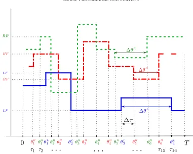
Let us recall that the duration of each heartbeat can be obtained as an RR-interval, which is the time interval between two successive R-waves registered by the ECG, see Fig.1.

Figure 1. Illustration of RR signal measurement

Next, we can precisely measure the time of each maximum of R-wave, and we denote it by ti. Then, the duration of the it_{hheartbeat is exactlyX}

i =ti−ti−1. The instantaneous heart rate (HR) is provided by the

equationHR= 60/RR, whereRR=X(ti) is measured in seconds,HR is measured in beats per minute. For biological reasons, the human HR is within the interval [20,250]bpm (beats per minute), i.e.,X(t) belongs to the RR interval 60/250s. < X(t)<60/20s.In real life situations, it is quite natural to consider nychthemeron activities as a sequence of more or less active periods (sleep, rest, stress,. . . ). This leads to modeling RR-series

X(ti) by locally stationary processes for both time and frequency domains.

Therefore, we assume that the signal is the sum of a piecewise constant function and a Gaussian process, centered and locally stationary. We then have the following representation:

X(t) =µ(t) +

Z

R

eitξpf(t, ξ)dB(ξ), for allt∈R, (1)

where

• B(ξ) is a ”well-balanced” Wiener measure, such thatX(t) is a real number, for all t∈R, see e.g. [18]

or [3] [2], for a precise definition.

• the function t 7→ µ(t) is also piecewise constant for another partition ˜τ1, . . . , τ˜L with µ(t) = µ` if

t∈[˜τ`,τ˜`+1 [.

The first step of data processing treated in this work will be the detection of instants where the parameters of the processX(t) will present an abrupt change in either time or frequency components.

Change points detection: the FDpV method

Change points detection is well studied in literature, we cite among others [5, 6]. The classical proposed solutions are usually based on penalized least square techniques which suffer from memory complexity and time consuming calculations. To overcome this problem Bertrand et al. [6] introduced a faster technique. The main idea of the FDpV method is based on two steps, the first consists in detecting changes without worrying about false detections, the second one consist in performing statistical test to remove false change points. The FDpV method has a theoretical complexity of orderO(n) while classical approaches are of orderO(n2). This technique have been optimized and coded with a java software and is able of making real-time detection.

Time-frequency analysis in HF and LF bands

According to recommendations of the Task force [7], we use the following notations :

• [ω1, ω2] = (0.04Hz, 0.15Hz) denotes the orthosympathetic frequency band;

• [ω2, ω3] = (0.15Hz, 0.5Hz) denotes the parasympathetic band

In order to efficiently extract energies corresponding to HF and LF bands we use techniques presented in [1] or [4]. Indeed they have introduced a theoretical study of the wavelet coefficients for stationary (or with stationary increment) centered Gaussian processes, i.e., for X given by (1) with µ(t) = 0. They have also generalized this result to locally stationary Gaussian processes. We give here a brief description of their technique: using a suitable wavelet, they extract the energies associated with LF and HF bands and localized around the timeb. This is measured by the modulus of the complex wavelet coefficients|Wi(b)|2 fori= 1,2, with

Wi(b) =

Z

R

ψi(t−b) X(t)dt,

whereψ1andψ2are suitable wavelets chosen with disjoint frequency supports corresponding to the LF and HF

bands. These wavelet coefficients are then computed at each second, i.e., the difference between two consecutive values for bis equal to 1 second.

Then we consider the change point problem of the mean of the multivariate time seriesZ1(b),Z2(b) where

Z1(b) = log |W1(b)|2

, and Z2(b) = log |W2(b)|2

, (2)

and we use a simple method well suited for big datasets, that is the Filtered Derivative with p-value (FDpV) method [6, 16].

How to choose the wavelets ψ1 andψ2 ?

In the idealistic case, we would use two filters ψ1 and ψ2 with compact support, the Fourier transforms

of which have support inside the orthosympathetic and parasympathetic bands. Unfortunately, there is no function ψ with compact time domain support and compact frequency support, see for instance [17, Th 2.6 p.34] . Therefore, the best we can do is to choose between a filter with a compact frequency support and a filter with a compact time domain support. The first choice is well suited for stationary models [2]. The price to pay for the compactness of the time domain support is the loss in the compactness of the frequency support. To evaluate the effect of the compactness loss, Ayache and Bertrand [1] have introduced the notion of

be compact1_{. The idea is then to adjust the pseudo support inside a specified frequency band whereρis close}

to 1. We have proposed a generic method permitting to find such supports by scaling and modulation [3]. For the sake of readability, let us recall the following proposition:

Proposition 1.1. Let ψbe a filter with compact support[L1, L2] and a frequencyρpseudo support[Λ1, Λ2].

Let us consider an arbitrary frequency band[ω1, ω2]and denote,

λ= ω2−ω1

Λ2−Λ1

, η=ω1+ω2

2 −(ω2−ω1)

Λ2+ Λ1

Λ2−Λ1

.

Then the map ψ1(t) = µ×eiηtψ(λt) with µ >0 has a ρ pseudo support [ω1, ω2] and a time domain support

_Λ

2−Λ1

ω2−ω1

L1,

Λ2−Λ1

ω2−ω1

L2

.

Proof. Since ˆψ1(ξ) =µ×ψˆ(

ξ−η

λ ), one can deduceρpseudo suppψ1=η+λ×ρpseudo suppψand then the

proposition.

The different choices for the filtersψ1andψ2are enlightened by Proposition 1.1. For computational reasons,

we will use the Gabor wavelets2defined as

ψ(t) =eiηtg(t) where g(t) = 1 (σ2_π)1/4e

−t2

2σ2 (3)

see for instance, [17]. This wavelet has the same time and frequency ρpseudo support [−L, L] = [−3.5,3.5] withρ= 0.9995. In the spectral domain, we have

ˆ

ψ(t) = ˆg(ξ−η), gˆ(ξ) = (4πσ2)1/4e−σ

2_ξ2

2 (4)

By using Prop. 1.1, we can fit the Gabor wavelet inside the orthosympathetic band, respectively the para-sympathetic frequency one. We obtain the two Gabor wavelets defined by (3) with the following choice of parameters:

η1=

ω1+ω2

2 and σ1=

2L

ω2−ω1

(5)

η2=

ω2+ω3

2 and σ2=

2L

ω3−ω2

(6)

Moreover|ρpseudo Suppψ1|=

4L2

ω2−ω1

and|ρpseudo Suppψ2|=

4L2

ω3−ω2

withρ= 0.9995. Fig. 3 displays

the Gabor wavelets coefficients in the orthosympathetic and parasympathetic bands respectively for the sample plotted in Fig.4.

1.2.

Classification and extraction of homogeneous HR profiles

Cluster analysis has been widely studied and used in many applied areas such as medicine, chemistry, social studies and psychology. Its main purpose is to identify groups or clusters present in the data. Clustering algorithms can be divided into two main categories: hierarchical methods and partitioning methods. Hierarchical methods are stepwise and either agglomerative or divisive. For instance ifnobjects have to be clustered, then in each step, two clusters are chosen and merged. This process continues until all objects are clustered into one

1_{Let0< ρ <1, a mapg∈L}2₍

R) andIcompact interval. The mapghave aρpseudo support if R

I|g(t)|

2_dt

R

R|g(t)|

2_dt =ρ.

2_{In [3] Daubechies wavelets have been investigated, they give similar results but cost more computation time. Using the Gabor}

group. On the other hand, divisive methods begin by putting all objects in one cluster. In each step, a cluster is chosen and split up into two. This process continues untilnclusters are produced. While hierarchical methods have been successfully applied to many biological applications (e.g. for producing taxonomies of animals and plants [15]), they are well known to suffer from the fact that they can not undo what was decided previously.

Principal component analysis (PCA) is a powerful tool for analyzing the correlations between several variables. It provides new uncorrelated components with higher informative power; combining the PCA with a hierarchical cluster analysis will overcome the evident strong correlation between the studied variables.

Let us denote ΘR = (θR

1 < θ

R

2 <· · ·< θ

R

m), Θ

L = (θL

1 < θ

L

2 <· · ·< θ

L

n) and Θ H

= (θH

1 < θ

H

2 <· · ·< θ

H p ) the change points of respectively theRRseries, the LF and HF energies. We gather these change points sequences inT = ΘR∪ΘL∪ΘH. Let us consider the ordered instantsT =τ1< τ2<· · ·< τM ofT whereM ≤m+n+p. We will be interested in the following variables:

• The variableθR

i −θ

R

i−1which represents the time lapse where the RR signal has a stationary behaviour.

• The variable θH_i −θH_i−1 which represents the duration of theith level of the HF energy. This duration can be seen as the duration where only the parasympathetic (braking) system is activated and has a fixed regime.

• The variable θL

i −θ

L

i−1 which represents the duration of theithlevel of the LF energy. This duration

can be seen as the lapse of time where only the orthosympathetic (acceleration) system is in action and has established a fixed regime.

• the variable τi−τi−1 which represents the interRR, HF andLF durations of the ith level of the HF

energy before one of the two systems switches to another state.

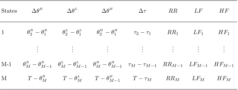
For a given individual we will construct a table that describes different states of the heart rate variability during the measurements. In this case we will have M states, for each we have the durations, ∆θR

, ∆θH , ∆θL

and ∆τ. On this lapse of time there is at least one change of the heart rate behaviour. This can be represented by the following table:

States ∆θR

∆θL

∆θH

∆τ RR LF HF

1 θR

2 −θ

R

1 θ

L

2 −θ

L

1 θ

H

2 −θ

H

1 τ2−τ1 RR1 LF1 HF1

..

. ... ... ... ... ... ...

M-1 θR

M −θ

R

M−1 θ

L

M −θ

L

M−1 θ

H

M −θ

H

M−1 τM−τM−1 RRM−1 LFM−1 HFM−1

M T−θR

M T−θ

L

M T−θ

H

M−1 T−τM RRM LFM HFM

Table 1: Presentation of the variables used for PCA projection and clustering.

In order to illustrate how the discriminating variables will be constructed, we give a simple example in Fig.2.

2.

Real case analysis

+ + + + + + + + + + + + + + + + + +

Figure 2. Illustration on how we construct the variables ∆τ,∆θ

of HR activity during a 24-hour shift. For this purpose, we make a blind separation of groups that highlights nychthemeral cardiac behaviour. Though we dispose of larger data sets with ECG measurements, we only focus on one emergency physician to show the efficiency of our approach. A further discriminant analysis will be investigated for the whole data collected from all 19 emergency physicians’ measurements. The idea is to give a theoretical framework that will be used to classify a cohort of emergency physicians.

2.1.

Data description

Algorithm 1: Data preprocessing for the construction of table1

Input: Cleaned RR signalX(t) on time interval [0, T]

Findb0 andbf first and last possible instant for which wavelets transform can be calculated.

foreach b=b0. . . bf do

- Calculate the log-energiesZ1(b) andZ2(b) given in (2) by using Gabor waveletsψ1 andψ2.

- Apply the FDpV method on theRRcleaned signalX(t) to extract (θR_i ) and the corresponding (RRi)

- Apply the FDpV method to (Z1(b), b=b0...bf) and extract (θ L

i) and its (LFi)

- Apply the FDpV method to (Z1(b), b=b0...bf) to extract (θHi ) and the corresponding (HFi)

Deduce the differences ∆θR , ∆θL

, ∆θH

Output: Variables ∆θR , ∆θL

, ∆θH

, mean RR, LF and HF

The output of the last algorithm creates the table 1, in which we consider the columns as the discriminating variables of the heart activity states.

2.2.

Results and graphical representations

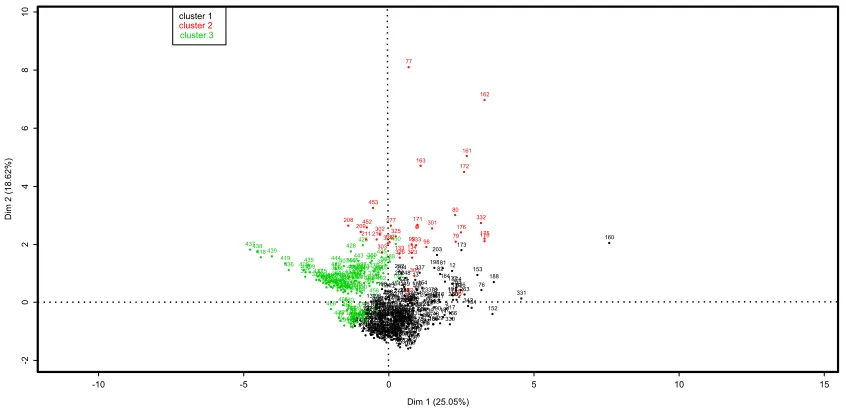
At first glance, we can realize that variables, given in table 1, are correlated and should be reduced to a lower dimension. For this reason we will perform the classification on the principal components instead of the initial data. The idea is to get rid of dependence or correlation between the initial variables and benefit from their orthogonality. After the PCA has been performed we make a hierarchical classification on the resulting principal components. Fig. 3 highlights three distinct clusters reflecting the heart rate behaviour of the studied individual.

-10 -5 0 5 10 15

-2 0 2 4 6 8 10

States clustering on principal components projections of table 1

Dim 1 (25.05%)

Dim 2 (1

8.62%) 437438 418 439 419 436 408 371410 435 409

372417370396415369420447241₂₀₇374411373

468 416 403392414397 366 429 444 375 395421393 434 473 431 386 37 401 412 367 466 448 471 206 407 399 291 385 368 432 440 462 208 398 460 376 451 464 355 390 244 424 428 394 240 467 476 406 16 290 5557 433 445 36 469 287 446 430 38 459 381 228 242 400 363 442 463 443 391 213 405 14 422 365 404 209 58 427 477 130 245 426 472 314 455 54 449 212 413 423 318 457 211 52 34 56 102 475 452 461 470 474 137 382361 481 380 59 236 224 345 131 223 15 292 103 389 480 379 39 377 273 453 320 142 378 456

275267316 219 288196200

383 465 197 210 353 125₅₃ 384 23 17 195 9 231 282 441 362 107 294214 138 285 234 302 319 458 45 23524 192 260 402 321 35 243 387 226 425 141 101 303 108 322 91 113 237 356 286 49 65 22 205 340 308 281 18 293 317 315 246 313 124 364 339 47 220 271 193 104 184 324 258 229 221 268 479 346 328 22748 359 109 40 132 388 42 143 112 289 277 218 67 327 93 262 129 13564 126 278 128 304 280 92 95 148 183 139 147 105 347 144 295 34150 354 450 454 325 296 26461 357 33 106 261 8 312 349 41 199 297 257 3 276 44 270 150 274 306 68 19 352 133 222 201 202 279 12787 149 326 350338 46 253 185₄ 158 140 225 30 89 204 478 20 51 239 35863 145 72 114 25 62 123 146 26 7 117 122 284 249 248 232 21 2 1 255 360 351 75 247 182 84 167 252 115 309 90 120 159 77 180 181 28 269 215 100 266 311 118 96 169 157 230 134 335 256 99 216 323 156 88 71 329 272 334 119 305 194 299 165 60 13 74 310 333 254 110 94 307 171 10 83 111 70 337 85 73 163 348 168 154 344 27 121 259 97 69 233 98 283 6 136₆₆ 86 301 238 343 186189 78 155 198 298 32 43 190 203 116 29 82 31 81 11 187 164 5 330 217 12 166 191 177 178 250 80 79 179 265 300 174 251336 176 173 172 263 161 342151 153 332 76 175 162 170 152 188 331 160 cluster 1 cluster 2 cluster 3

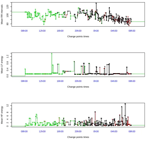
In order to locate each cluster in the RR, HF and LF during the activity day timeline, we reproduce the mean signals and their corresponding change points. In Fig. 4, we see clearly what happens to the autonomous nervous system activity. We recognize in Fig. 4 the specific behaviour of the autonomic nervous two opposite systems(parasympathetic and orthosympathetic); it is reflected here by an alternation of the low and high frequency energies. This type of classification suggest that it would possible to extract an indicator of stress or well-being by comparing the occurrence of this clusters to the actual feeling of the physician during his shift.

80

100

120

Change points times

Mean RR inter

v als ●●● ● ● ● ● ● ● ● ●● ●● ● ●●● ● ● ● ● ● ● ●●●● ● ● ● ● ● ● ● ●●●● ●● ● ●● ● ● ● ● ●●● ● ● ●● ● ● ●● ● ●●●●● ● ●●_●●● ● ● ● ● ●●● ●●●●●●●● ● ● ●● ● ● ● ●●●●● ●● ● ● ●● ●● ●●●● ● ●●●● ●●●● ●● ● ●● ● ● ● ● ● ● ● ●● ●●●● ●●● ● ●_● ●● ● ● ●● ● ● ●● ● ● ●● ● ● ●●● ●●● ● ● ● ●●● ● ● ●●●●●● ● ●●● ●●● ●●●●● ● ●●●●● ● ● ● ● ● ●●●● ● ● ● ● ●●●●● ● ● ●●●● ● ●● ● ● ●● ●● ● ● ● ● ●●● ● ● ● ● ●● ●●● ● ● ● ●● ● ● ● ●●●● ● ● ●●●● ● ● ●● ● ● ● ●●●● ● ● ● ● ● ●●● ● ● ●● ● ● ● ● ● ● ●● ● ● ●● ● ● ● ●●●●●●●● ●●● ● ● ● ● ● ● ● ● ●● ● ● ●● ● ● ●●● ●● ●● ● ● ● ●● ● ● ● ●● ●●● ● ● ● ● ●● ●●● ● ●●● ● ● ●● ● ● ● ● ● ● ●●●● ● ● ● ●● ● ● ● ● ● ● ● ● ● ● ●● ● ● ● ● ● ● ● ● ● ● ●● ● ● ● ● ●●● ● ● ● ● ● ● ●●●● ● ●● ● ●● ●● ●● ●●● ● ● ● ●●_● ● ●● ● ● ●● ● ●●● ● ● ●●● ● ● ● ● ● ●● ● ● ● ●● ● ● ● ● ● ● ●● ●● ● ●

08h30 12h30 16h30 20h30 0h30 04h30 08h30

0.0

0.4

0.8

1.2

Change points times

Mean LF energy

● ●● ●●●●●● ●●●●●●●●●●●●●●●●●●●●●●●●●●●●●●●●●●●●●● ●●●●●●●●●●●●●●●●●●● ●●●●●●●●●● ● ● ● ● ● ●●●●●●●●●●●● ●●●● ● ● ●●●●● ●●● ●●●●●●● ●●●●●● ● ● ●● ● ● ● ●●●● ● ● ● ● ●●●●●●●● ●●●●●●●●●●●●●●●●● ● ● ● ●●●●●● ●●● ● ● ●● ●●●●●●●●●●●●●●●●●●●●●●●●●●●●●●● ●●●● ● ●●●●●●●●●●●●●●●●●●●●●● ●●●●●●●●●●●●● ● ●● ●● ● ● ●●●●●●● ●●●●●●●●●●●●●●● ● ●●●●●●●●●●●●●●●● ●●●●●●● ● ● ● ● ● ●●●●●●●●●●●●●●●●● ● ●●● ● ● ●●● ● ● ● ●●●●●●●●●●●●●●●●●●●●●●●●●●●●●●●●●●●●●●●●●●●●●●●●●●●●●●●●●●●●●●●●●●●●●●●●●●●●●●●●●●●●●●●●●●●●●●●●●●●●●●●●●●●●●●●●●●●●● ●● ● ●●●●●●●●● ● ● ● ●●●●●●●●●●●●●●●

08h30 12h30 16h30 20h30 0h30 04h30 08h30

0 2 4 6 8 12

Change points times

Mean HF energy

●● ● ●●●●●● ●● ● ● ● ●● ● ● ● ●●●● ●● ● ● ●●● ● ●● ● ●● ● ● ● ● ● ●●●● ●● ● ●●●●●● ●●●● ●●●● ● ● ●● ● ● ●● ● ●● ●●●●● ● ●●● ● ● ●●● ●● ● ●● ● ● ●● ● ● ●●● ● ● ● ● ● ●● ●●● ●● ●●● ● ● ● ●●●● ● ● ● ● ● ● ● ● ● ● ●● ● ● ● ● ●●●● ● ● ● ● ● ● ●●● ●●● ● ● ● ●●● ● ●● ●●● ● ●● ● ● ● ●● ● ● ●●● ●● ●● ● ●● ● ● ● ●● ●_●● ● ● ●●●●●●● ● ● ● ●● ●●● ● ●●●●● ● ●●●●●●● ● ● ● ● ● ●●● ● ● ● ●● ●●● ● ● ● ●●● ●●●●●●● ● ● ●●● ●● ● ●●●● ● ● ●●●● ● ●●●●● ●● ●●●● ● ●● ● ● ●● ● ● ● ● ●● ●●●●●●●● ● ●● ●● ● ● ● ●●●●● ●● ●● ● ●●●●●●●●●●● ● ● ● ● ● ●●●●●_●●● ●●●●● ● ● ● ● ●●●●●●● ● ●● ●● ●●● ● ● ● ●●●●●●● ●●●●● ●● ●●● ● ● ●●● ● ●●●●●● ● ● ● ●●● ● ●●● ●●● ● ● ● ● ● ● ● ● ● ● ● ● ● ● ●● ● ● ● ●●● ●●● ● ● ● ● ● ● ● ● ● ●●●● ● ● ●● ● ●● ●●● ● ●● ● ●●●●●●● ●●●●●

08h30 12h30 16h30 20h30 0h30 04h30 08h30

We can also quantify the discriminating power of each variable on the classification. Doing so, we determine what characteristics explain most cluster differentiations.

3.

Conclusions

We introduce a methodological approach highlighting the action of the autonomous nervous system on the heart rate activity during a 24-hour shift of an emergency physician. The use of spectral analysis with Gabor wavelets permits to extract energies corresponding to high and low frequency bands. The resulting energies are used to construct discriminating variables that reflect the way heart rate is modulated by the emergency physician activity.

Further research should be conducted on a large number of individuals. The classification results will be combined with a survey concerning emergency physician real feel during their shift. This will allow to extract stress or well-being indicators.

References

[1] A. Ayache and P. R. Bertrand,Discretization error of wavelet coefficient for fractal like processes, Advances in Pure and Applied Mathematics, 2 (2011), pp. 297–321.

[2] J.-M. Bardet and P. Bertrand,Identification of the multiscale fractional brownian motion with biomechanical applications, Journal of Time Series Analysis, 28 (2007), pp. 1–52.

[3] J.-M. Bardet and P. R. Bertrand,A non-parametric estimator of the spectral density of a continuous-time gaussian process

observed at random times, Scandinavian Journal of Statistics, 37 (2010), pp. 458–476.

[4] J.-M. Bardet, H. Bibi, and A. Jouini,Adaptive wavelet-based estimator of the memory parameter for stationary gaussian

processes, Bernoulli, 14 (2008), pp. 691–724.

[5] M. Basseville and I. Nikiforov, Detection of abrupt changes: Theory and application. 1993, Information and System

sciences, Prentice-Hall.

[6] P. R. Bertrand, M. Fhima, and A. Guillin, Off-line detection of multiple change points by the filtered derivative with

p-value method, Sequential Analysis, 30 (2011), pp. 172–207.

[7] A. Camm, M. Malik, J. Bigger, G. Breithardt, S. Cerutti, R. Cohen, P. Coumel, E. Fallen, H. Kennedy, R. Kleiger, et al., Heart rate variability: standards of measurement, physiological interpretation and clinical use. task force of the

european society of cardiology and the north american society of pacing and electrophysiology, Circulation, 93 (1996), pp. 1043–

1065.

[8] A. Chamoux and P. Catalina,Le syst`eme holter en pratique, M´edecine du Sport, 58 (1984), pp. 43–273.

[9] M. O. Diab, C. Marque, and M. A. Khalil, Classification for uterine emg signals: Comparison between ar model and

statistical classification method, INTERNATIONAL JOURNAL OF COMPUTATIONAL COGNITION (HTTP://WWW.

IJCC. US), 5 (2007).

[10] F. Dutheil, G. Boudet, C. Perrier, G. Lac, L. Ouchchane, A. Chamoux, M. Duclos, and J. Schmidt,Jobstress study: Comparison of heart rate variability in emergency physicians working a 24-hour shift or a 14-hour night shift a randomized

trial, International journal of cardiology, 158 (2012), pp. 322–325.

[11] F. Dutheil, M. Trousselard, C. Perrier, G. Lac, A. Chamoux, M. Duclos, G. Naughton, G. Mnatzaganian, and J. Schmidt,Urinary interleukin-8 is a biomarker of stress in emergency physicians, especially with advancing age the

job-stress* randomized trial, PloS one, 8 (2013), p. e71658.

[12] U. Frisch,Turbulence, Turbulence, by Uriel Frisch, pp. 310. ISBN 0521457130. Cambridge, UK: Cambridge University Press,

January 1996., 1 (1996).

[13] A. Goldberger,Heartbeats, hormones and health : is variability the spice of life ?, Am. J. Crit. Care Med, 163 (2001),

pp. 1289–1290.

[14] P. C. Ivanov, L. A. N. Amaral, A. L. Goldberger, S. Havlin, M. G. Rosenblum, Z. R. Struzik, and H. E. Stanley,

Multifractality in human heartbeat dynamics, Nature, 399 (1999), pp. 461–465.

[15] L. Kaufman and P. J. Rousseeuw,Finding groups in data: an introduction to cluster analysis, vol. 344, Wiley. com, 2009. [16] N. Khalfa, P. R. Bertrand, G. Boudet, A. Chamoux, and V. Billat,Heart rate regulation processed through wavelet

analysis and change detection: Some case studies, Acta biotheoretica, 60 (2012), pp. 109–129.

[17] S. Mallat,A wavelet tour of signal processing. 1998.