3-DIMENSIONAL ANALYTICAL SOLUTION FOR LUNAR DESCENT SCHEME

(1)

Printed in The Islamic Republic of Iran, 2015 © Shiraz University

3-DIMENSIONAL ANALYTICAL SOLUTION FOR

LUNAR DESCENT SCHEME

*

I. M. MEHEDI

1**

, T. KUBOTA

2

AND U. M. AL-SAGGAF

3

1,3_{Center of Excellence in Intelligent Engineering Systems (CEIES), King Abdulaziz University, Jeddah,}

Saudi Arabia

1,3_{Electrical and Computer Engineering Department, King Abdulaziz University, Jeddah, Saudi Arabia}

2_{The University of Tokyo, Tokyo, Japan}

Email: [email protected]

Abstract–Lunar and Mars landing is a crucial part of any exploration mission. Its importance is manifested by the considerable interest in the past couple of decades. Solution of lunar descent can be either numerical or analytical. Numerical solutions are iterative and computationally demanding and some of them might not be suitable for on-board implementation. On the other hand, analytical solutions are not complex and are much more attractive for the same purposes. All the present analytical solutions schemes are two dimensional considering only altitude and down range to describe the reference trajectories of a lunar descent. The main contribution of this paper is the development of 3-dimensional analytical solution for the reference trajectory which is crucial for a precise landing of a lunar spacecraft. In this investigation cross range distance is incorporated for complete representation. Comparisons are made by simulated responses between numerical and analytical solutions. Detailed mathematical derivations are presented in this paper as well.

Keywords– Lunar descent, numerical solution, analytical solution, 3-D modeling

1. INTRODUCTION

Lunar and Mars landing is a crucial part of any exploration mission. Its importance is manifested by the considerable interest in the past couple of decades [1-10]. For a lunar lander, it is essential that the landing on the lunar surface is vertical and soft. A scheme to fulfill this requirement is the gravity-turn descent that has been used for both lunar and Mars probes [1], [2], [11-14]. In this descent technique, the lander thrust vector is maintained opposite to the instantaneous velocity vector along the descent path [15]. The great benefit of gravity-turn descent is that the landing is assured to be vertical and the guidance law is close to fuel optimum [3].

Lunar guidance takes a horizontally oriented spacecraft from orbital speeds, hundreds of kilometers from the desired landing point, to a very low speed and an almost vertical orientation. Guidance schemes for lunar landing date back to the Apollo era [4], [5]. The Apollo lunar descent guidance schemes worked well to meet the criteria of the 1960s. However, they cannot fulfill the demanding goals of future lunar exploration that encompasses the desire to explore several locations on the moon easily and cheaply.

In conventional gravity-turn descent guidance law, the solution of spacecraft equations of motion is numerical and iterative. Due to complexity, a numerical solution limits real time implementation. Therefore, it is impartial to seek an analytical solution. An analytical targeting solution can generate multi-dimensional trajectories on-the-fly and easily re-target the spacecraft to another landing site. At the end of the last century, a 2-dimensional analytical solution was developed for lunar landing mission [15] and [3].

_{Received by the editors January 16, 2014; Accepted May 5, 2015.} 

(2)

The same 2-dimensional concept is proposed in [16] based on an analytical solutions to the equations for down range and altitude but excluding cross range distance. However, in the literature and to date there is no result for a full analytical 3-dimensional spacecraft reference trajectory that includes cross range, altitude and down range distance. This gap in the literature is filled by the present paper. Authors have already investigated 2-dimensional schemes for lunar landing solution [16] and [17]. The preliminary investigation of 3-dimensional scheme is presented in the poster session of a conference [18] and in this paper a comprehensive treatment is performed. The main contribution of this research work is the development of a complete 3-dimensional analytical solution for the reference trajectory which is crucial for a precise lunar landing mission.

An advantage of numerical solutions is the ability to accommodate constraints in the state and control variables inherent in planetary landing optimal control problems. This advantage is offset by the fact that numerical solutions are iterative, computationally expensive and not suitable for on-board implementation. Nevertheless, some authors proposed solving an on-board nonlinear optimization problem [19]. Other authors tried to overcome the computational burden by solving a related problem that does not minimize fuel use [20], [31] and [32]. However, the applicability of nonlinear optimization approaches to on-board implementation is limited. This is due to the fact that with such techniques it is not possible to a have a priori knowledge of the required number of iterations needed to find a feasible trajectory and there is no guarantee of achieving the global optimum. Nevertheless, recent advances in convex optimization may remedy the problem. The applicability of such techniques for on-board implementation is made feasible by advances in computing power, modern algorithms and new coding techniques that exploit the structure of the given problem [21]. One of these approaches is described in [22] where approximate solutions to the minimum-fuel powered-descent guidance are formulated as a second order cone program (SOCP). This optimization problem can be solved in polynomial time using interior point-method algorithms [23-25]. For any given accuracy, the global optimum can be found with a priori upper bound on the required number of iterations needed to achieve the optimum. The limitation of the approach in [22] is that it assumes a feasible solution exists. This limitation is eliminated in [13] to handle the case when no feasible trajectory to the target exists. This approach is extended even further in [26] where lossless convexifications are used when the problem has nonconvex control constraints. Extensive comparisons of the convex optimization approach to alternative approaches are given in [27], [13], [26] and [28]. One last remark is that advances in computing power are not quickly implemented in the very expensive space

hardened microprocessors. The state of the art on-board processor is still the RAD750TM space hardened

microprocessor [29] and [30] that is identical in architecture, function, and operation to the commercial

IBM PowerPC750TM microprocessor. It is only 400 Dhrystone 2.1 MIPS at 200 MHz which is far behind

in performance when compared with the present desktop microprocessors.

(3)

2. 3-D STATE EQUATIONS

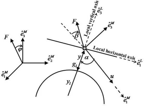
A lunar descent schematic diagram is shown in Fig. 1 where the local vertical local horizontal (LVLH)

reference frame is denoted by L. The figure also shows the relationship of the maneuver frame, denoted by

M, to the LVLH unit vectors.

Fig. 1. Lunar descent schematic diagram

The fundamental three dimensional equations of motion describing a spacecraft landing on a uniform sphere shaped lunar body [1] are divided into two parts. The first part describes the spacecraft dynamics and is given by the following equations:



 cos

cos )

( N

l g t

u   ₍₁₎

] cos sin sin

) [(

1 ) (

2

  

 g N

y y

u u

t _l

l

 

 

 ₍₂₎

] cos sin [ sin

1 )

(  



 N

u t 

 ₍₃₎

Where u is spacecraft velocity vector magnitude or spacecraft speed, gl is lunar gravitational

acceleration, N is ratio of thrust F and vehicle mass m, α is pitch angle of the vehicle velocity vector

relative to the local vertical, β is angle of thrust vector relative to reverse direction of spacecraft velocity, y

is altitude of the spacecraft from lunar surface, ylis lunar radius, ψ is cross range angle, and φ is thrust roll

angle.

The second part describes the kinematics and is given by the following equations: 

cos )

(t u

y  (4)

l l

y y

y u

t x

  sincos )

(

 ₍₅₎

l l

y y

y u

t c

  sinsin )

(

 ₍₆₎

(4)

a) Preliminary postulation

Right hand sides of the spacecraft governing equations are reduced to function of velocity vector

pitch angle α. To do this we make some reasonable assumptions regarding thrust to mass ratio, thrust

vector angle and lunar gravitational acceleration force. To generate an ideal descent trajectory, it is

rational to assume constant values for N,i.e., F/m and gl, and control input β is set to zero. These are not

restricting assumptions since in the case of constant thrust acceleration, m will not be constant and thus

F/m will be varying but the error will be removed by the real time guidance algorithm. With these

assumptions, Eqs. (1) to (3) reduce to:

] sin ) [( 1 ) ( 2   _l l g y y u u t     (7) N g t

u() lcos (8)

0 ) (t 

 ₍₉₎

Therefore, ψ (t) is constant. Since landing must take place close to the lunar surface, consequently it is a

reasonable practical assumption that y << ylwhich implies that yl/y + yl ≈ 1. Using this in Eqs. (5) and (6)

gives:



cos

sin ) (t u

x  (10)



 sin

sin )

(t u c

c  (11)

3. 3-D NUMERICAL SOLUTION

To find a numerical solution during the powered descend phase, the above equations need to be simplified

and rearranged in a format suitable for a numerical solver. We derive the equations below for speed u,

time t, downrange x, altitude y and cross range c as a function of a single variable; namely the velocity

vector pitch angle α.

Using Eqs. (7) and (8), the equation for speed u is derived as follows:

    sin ) / ( ) cos ( ) ( ₂ l l l g y u N g u dt d dt du u      ₍₁₂₎ Then    d N g du g y u u l l l sin cos ) (

1 2 _ _ 

This can be integrated as:



        0 0 sin cos ) ( 1 2 d N g du g y u u l u u l l

Therefore, the equation for speed becomes:





2

1

)

( g yW

u   _l _l (13)

where the Lambert function W is expressed as:

l l l g N y g u l l e y g u W 2 ) ( 2 2 0 sin cos 1 sin 2 0               (14)

Using Eqs. (8) and (12), the descent time tD can be obtained by integrating the following equation

(5)

D D D dt du d du d dt t   )  (  ) ( ) ( t u u    ₍₁₅₎

Similarly, the equation for altitude can be rewritten as:

   d dt dt dy d dy y D D   ) (

 y(t)tD() (16)

Now substituting the values from Eq. (4) gives:

) ( cos )

( u t_D 

y   (17)

Where u can be replaced from Eq. (13). Similar procedure can be followed to express the horizontal

span as a function of the velocity vector pitch angle α.

) ( ) ( ) (   

 D D

D t t x d dt dt dx d dx

x      ₍₁₈₎

Using Eq. (10) gives:

) ( cos sin )

( u  t_D 

x   (19)

A similar procedure is applied to derive the following equation for the cross range:

) ( sin sin )

( u  t_D 

c  ₍₂₀₎

4. 3-D ANALYTICAL DESCENT SOLUTION

Here we derive a 3-dimensional full analytical solution for the lunar descent problem. We make the reasonable practical assumption that the lunar surface for this problem can be considered as a plane

surface. That is yl → ∞ so that the Eq. (7) now reduces to:



( ) sin

u g t  l

 ₍₂₁₎

This reduced equation is used to obtain a single, separable differential equation with α as the independent variable. From the above we have:

    sin ) cos ( ) ( / ) ( ) ( l l g N g u t t u

u     ₍₂₂₎

then 0 csc cot 1     

 gl

N d

du

u (23)

Now Eq. (23) can be integrated to obtain the descent speed u as a function of velocity vector pitch angle α

as [1] and [28]:

l g N u u _           ) 2 / tan( ) 2 / tan( sin sin ) ( 0 0 0 _     (24)

where, u0 and α0 are initial values for speed and velocity vector pitch angle, respectively.

Differentiating Eq. (24):

                           cot ) sin( ) 2 / tan( ) 2 / tan( sin sin ) ( 0 0 0 l g N g N u d du

u l (25)

(6)

range. First, the descent time is given as: D D D dt du d du d dt t   )  (  ₍₂₆₎

Using Eqs. (8) and (25) gives:

                         N g g N u t l l g N D l         cos 1 cot ) sin( ) 2 / tan( ) 2 / tan( sin sin ) ( 0 0 0  (27)

Similarly, the altitude is given as:

D D dt d dt dy d dy y   )  (  ₍₂₈₎

Using Eqs. (4), (21) and (25) gives:

                  l g N l g u g u

y l 

      cot ) 2 / tan( ) 2 / tan( sin sin cot ) ( 2 0 2 0 2 0 2  (29)

Using Eqs. (10) and (21), the down range distance is given as:

 

) cos

( 2 l D D g u dt d dt dx

x   (30)

 

 



 1 cos

) 2 / tan( ) 2 / tan( sin sin ) ( 2 0 2 0 2 0                   l g N g u

x l (31)

Similarly, using Eqs. (11) and (21), the cross range distance is given as:

 

) sin

( 2 l D D g u dt d dt dc

c   (32)

 

 



 1 sin

) 2 / tan( ) 2 / tan( sin sin ) ( 2 0 2 0 2 0                   l g N g u

c l (33)

a) Descent constraints

To compare the analytical and numerical solutions, parameters have to be specified. These specifications are shown in Table 1.

Table 1. Lunar descent constraints

Item Value

Lunar gravitational acceleration (gl) 1.623 [m/s 2]

Thrust to mass ratio (N ) 4 [N/kg]

Initial lander speed (u0) 1688 [m/s]

Initial velocity vector pitch angle (α0) 90 [deg.]

(7)

5. SIMULATION RESULTS

As can be seen from the previously derived equations, the cross range angle ψhas no effect on speeds,

time and altitude. As such, the trajectory responses for descent speeds, time and altitude are plotted in Fig. 2 as function of the velocity vector pitch angle α. For comparison, both the analytical and the numerical solutions are shown. The full integrated numerical solution is considered as an ideal solution and a benchmark for lunar descent trajectory and it is used to evaluate any other solution. However, it is to be noted that this method is complex, iterative and requires a long time to be executed and thus is not suitable for real time precise landing application. We will demonstrate that our analytical solution is close to this ideal numerical solution.

From Fig. 2, speed and time responses for both the numerical and analytical solution are almost similar. However, there is a difference in the altitude response as shown in Fig. 2d. From the figure, as the velocity vector pitch angle approaches zero, the analytical solution reaches closer to the surface than that of the numerical solution. This means that the analytical solution takes the spacecraft at lower altitude to initiate terminal descent.

0 10 20 30 40 50 60 70 80 90 0 200 400 600 800 1000 1200 1400 1600

Velocity vector pitch angle (deg)

H

o

ri

zo

n

ta

l

sp

ee

d

(m

/s

ec

)

Numerical Solution Analytical Solution

0 10 20 30 40 50 60 70 80 90 0 50 100 150 200 250

V

er

ti

ca

l

sp

ee

d

(m

/s

ec

)

(a) (b)

0 10 20 30 40 50 60 70 80 90 0 50 100 150 200 250 300 350 400 450

Velocity vector pitch angle alpha(deg)

T

im

e(

se

c)

0 10 20 30 40 50 60 70 80 90 -90 -80 -70 -60 -50 -40 -30 -20 -10 0 10

V

er

ti

ca

l

ra

n

g

e(

k

m

)

(c) (d)

Fig. 2. Comparison of numerical solution to analytical solution: Speed, Time and Altitude

(8)

0 10 20 30 40 50 60 70 80 90 -0.1

0 0.1 0.2 0.3 0.4 0.5 0.6 0.7

Velocity vector angle(deg)

C

ro

ss

r

an

g

e(

k

m

)

Crossing angle=0.0 & 0.1(deg)

Numerical solution Analytical solution

0 10 20 30 40 50 60 70 80 90 0

0.5 1 1.5 2 2.5 3 3.5

C

ro

ss

r

an

g

e(

k

m

)

Crossing angle=0.5(deg)

Numerical solution Analytical solution Crossing angle = 0.1(deg)

Crossing angle = 0.0(deg)

Fig. 3. Cross range response with respect to velocity vector pitch angle

The cross range angle is an important factor for precise lunar landing mission. In previous investigations, 2-D lunar descent trajectories are designed considering only the altitude and down range distance. In these investigations, the assumption of zero cross range angle is made [3], [16]. With such assumption, the cross range travel will be zero. Thus the important cross range distance parameter is overlooked. But as can be seen from Fig. 3, the trajectory is very sensitive to the cross range angle. A small cross range angle of 0.1 degrees can result in more than 600 m cross range travel and if the angle is 0.5 degrees, the landing spacecraft moves more than 3 [km] from the line of down range.

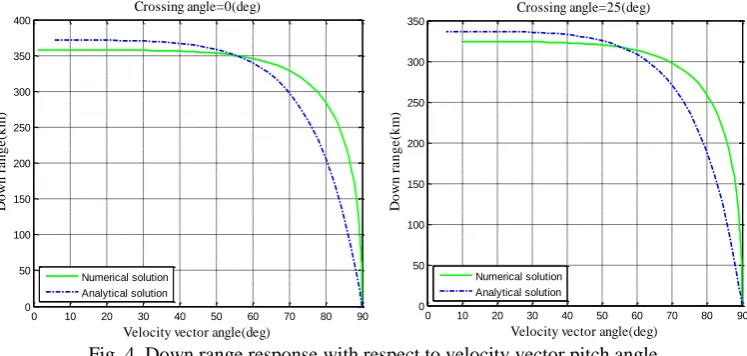
The above analysis proves that the 3-D analysis, including cross range angle, is influential in trajectory design for precise lunar landing missions which was absent in conventional 2-D trajectory designs. Moreover, it is not only the cross range distance that is affected by changes of the cross range angle. The down range distance is also influenced. Figure 4 shows the simulation results for down range response of both numerical and analytical solutions as a function of velocity vector pitch angle α. The figure shows that an increase in the cross range angle will result in a decrease of the down range distance. As a result, the lunar landing spacecraft will travel a shorter distance than required. A cross range angle increase of up to 25 degrees will result in down range distance decreases of more than 30 [km] as shown in Fig. 4.

0 10 20 30 40 50 60 70 80 90

0 50 100 150 200 250 300 350 400

D

o

w

n

r

a

n

g

e

(k

m

)

Crossing angle=0(deg)

0 10 20 30 40 50 60 70 80 90

0 50 100 150 200 250 300 350

D

o

w

n

r

a

n

g

e

(k

m

)

Crossing angle=25(deg)

Fig. 4. Down range response with respect to velocity vector pitch angle

(9)

small errors of cross range and down range can be eliminated by using real-time guidance scheme during the descent.

6. 3-D RESPONSE

Sections 3 and 4 described a detailed 3-dimensional mathematical modeling of a lunar landing mission. Numerical and analytical solutions are derived and a computer simulation is performed. Figure 5 shows the trajectories for both the numerical and analytical solutions. In the simulation, the constant values

shown in Table 1 are used for lunar gravitational acceleration gl, thrust to mass ratio N, initial vehicle

speed u0 and initial velocity vector pitch angle α0. Simulation is performed for different values of cross

range angle and specially observed here for two cases. Figures show the impact of including crossing angle in this 3-dimensional investigation. The changes in crossing angle surely affect the pinpoint landing mission. Further, the down range distance will also be affected due to the different values of cross range angle. It is also observed that the altitude is not affected at all by changing the cross range parameter.

The simulation shows that the trajectories of the less complex analytical solution always follow the response of ideal but complex numerical solution. As shown in Fig. 5, the altitude of analytical solution is maintained 40 km lower than the numerical solution. This low altitude flight path may assist the lunar landing spacecraft to activate terrain based navigation devices for hazard avoidance and safe landing.

To better understand the complexity of the numerical solution, we compare the execution time of both the numerical solution and the analytical solution. Table 2 shows the execution time of both schemes when a dual core 2.66 GHz computer is used as a computational platform. This old desktop computer is 13.33 times faster than the current available on-board computer which is only 200MHz [29] and [30]. Table 3 shows a simulated executing time of the on-board flight computer. According to this elapsed time analysis, the proposed 3-dimensional analytical solution has an execution time that is significantly less than that for the fully integrated numerical solution. The analytical solution is more than 140 times faster than the complete numerical solution.

Table 2. Elapse time comparison using laboratory desktop computing [second]

Numerical Solution 3D Analytical Solution

4.22 0.03

Table 3. Simulated elapse time comparison for on-board computer [second]

Numerical Solution 3D Analytical Solution

56.25 0.40

0 20

40 60

80 100

0 100

200 300

400 -100

-80 -60 -40 -20 0

Cross Range (km) Down Range (km)

A

lt

it

u

d

e

(k

m

)

0 50

100 150

200 250 0

100 200

300 400 -100

-80 -60 -40 -20 0

Cross Range (km) Down Range (km)

A

lt

it

u

d

e

(k

m

)

(a) Crossing angle = 50 (b) Crossing angle = 200

(10)

7. CONCLUSION

In this paper, full 3-dimensional numerical and analytical solutions are derived for lunar descent and compared in a simulation study. This is the first time in the literature that a complete analytical 3-dimensional solution is derived as compared to the frequently adopted simplifying assumption of a 2-dimensional trajectory. Simulation results show that the numerical and analytical solutions are almost similar except for the altitude. This low altitude flight path of the analytical solution may assist the lunar landing spacecraft to activate terrain based navigation accessories for hazard avoidance and safe landing. In the proposed scheme, the availability of the descent velocities, time, altitude, down range and cross range as a function of the velocity vector pitch angle can be utilized to reduce the computational burden on real-time lunar descent guidance algorithms for future precise landing missions.

Acknowledgements: This article was funded by the Center of Excellence in Intelligent Engineering

Systems (CEIES), King Abdulaziz University, Jeddah. Therefore, the authors acknowledge, with thanks, CEIES financial support. It was also supported by the facility of Japan Aerospace Exploration Agency (JAXA).

REFERENCES

1. Cheng, R. K. (1964). Lunar terminal guidance. In Lunar Missions and Exploration, edited by C. T. Leondes and R. W. Vance, Univ. of California Engineering and Physical Sciences Extension Series, pp. 308-355. Wiley, New York.

2. Cheng, Y. H., Meredith, C. M. & Conrad, D. A. (1966). Design considerations for surveyor guidance. Journal of Spacecraft and Rockets, Vol. 3, No. 11, pp. 1569–1576.

3. McInnes, C. R. (2003). Gravity-turn descent from low circular orbit conditions. Journal of Guidance Control and Dynamics, Vol. 26, No. 1, pp. 183–185.

4. Klumpp, R. A. (1971). Apollo guidance, navigation, and control: Apollo lunar-descent guidance. Technical report, MIT Charles Stark Draper Laboratory.

5. Klumpp R.A. Apollo lunar descent guidance. Automatica, 10(2):133–146, 1974.

6. Ueno, S. & Yamaguchi, Y. (1998). Near-minimum guidance law of a lunar landing module. 14th IFAC Symposium on Automatic Control in Aerospace. pp. 377–382.

7. Sostaric, R. (2006). Lunar descent reference trajectory. Technical report, NASA/JSC.

8. Xing-Long, L., Gaung-Ren, D. & Kok-Lay, T. (2008). Optimal soft landing control for moon lander. Automatica, 44:1097–

1103.

9. Chao, B. & Wei, Z. (2008). A guidance and control solution for small lunar probe precise-landing mission. Acta Astronautica, Vol. 62, pp. 44–47.

10. Feng, Z. & Gaung-Ren, D. (2013). Integrated translational and rotational control for the terminal landing phase of a lunar module. Aerospace Science and Technology, Vol. 27, No. 1, pp. 112–126.

11. Braun, R. D. & Manning, R. M. (2007). Mars exploration entry, descent and landing challenges. Journal of Spacecraft and Rockets, Vol. 44, No. 2, pp. 10–323.

12. Lutz, T. (2010). Application of auto-rotation for entry, descent and landing on mars. 7th International Planetary Probe Workshop.

13. Blackmore, L., Acikmese, B. & Scharf, D. P. (2010). Minimum landing-error powered descent guidance for mars landing using convex optimization. AIAA Journal of Guidance, Control and Dynamics, Vol. 33, No. 4, pp. 1161–1171.

14. ShangKristian,Y. H. & UldallKristiansen, P. L. (2011). Dynamic systems approach to the lander descent problem. AIAA Journal of Guidance, Control, and, Vol. 34, No. 3, pp. 911–915.

(11)

16. Mehedi, I. M. & Kubota, T. (2011). Advanced guidance scheme for lunar descent and landing from orbital speed conditions.

Transaction of Japan Society for Aeronautical and Space Sciences, Vol. 54, No. 184, pp. 98–105.

17. Mehedi, I. M. & Kubota, T. (2011). A trajectory generation scheme for precise and safe lunar landing. Journal of Space Engineering, Japan Society of Mechanical Engineering (JSME), Vol. 4, No. 1, pp. 1–13.

18. Mehedi, I. M. & Kubota, T. (2012). 3-dimensional analytical solution for lunar descent scheme. 63rd International Astronautical Congress 2012, Space Exploration Symposium Moon Exploration, Poster Session, Naples, Italy.

19. Topcu, U., Casoliva, J. & Mease, K. D. (2007). Minimumfuel powered descent for mars pinpoint landing. Journal of Spacecraft and Rockets, Vol. 44, No. 2, pp. 324–331.

20. Najson, F. & Mease, K. D. (2006). Computationally inexpensive guidance algorithm for fuel-efficient terminal descent.

Journal of Guidance, Control and Dynamics, Vol. 29, No. 4, pp. 955–964.

21. Mattingley, J. & Boyd, S. (2010). Real-time convex optimization in signal processing. IEEE Signal Processing Magazine, Vol. 3, No. 11, pp. 1569–1576.

22. Acikmese, B. & Polen, S. R. (1353). A convex programming approach to constrained powered descent guidance for mars pinpoint landing. AIAA Journal of Guidance, Control and Dynamics, Vol. 30, No. 5, pp. 1353–1366.

23. Sturm, J. F. (2002). Implementation of interior point methods for mixed semidefinite and second order cone optimization problems. Optimization Methods and Software, Vol. 17, No. 6, 1105–1154.

24. Sturm, J. F. (1999). A matlab toolbox for optimization over symmetric cones. Optimization Methods and Software, Vol. 11, No. 1, pp. 625–635.

25. Ye, Y. (1997). Interior Point Algorithms. Vol. 33. Wiley, New York.

26. Acikmese, B. & Blackmore, L. (2011). Lossless convexication for a class of optimal control problems with nonconvex control constraints. Automatica, Vol. 47, No. 2, pp. 341–347.

27. Steinfeld, B. A., Grant, M. J., Matz, D. A, Braun, R. D. & Barton, G. H. (2010). Guidance, navigation and control system performance trades for mars pinpoint landing. AIAA Journal of Spacecraft and Rockets, Vol. 47, No. 1.

28. Matthew, W. H. & Acikmese, B. (2014). Lossless convex- 8 ification of non-convex optimal control problems for state constrained linear systems. Automatica, Vol. 50, No. 9, pp. 2304–2311.

29. Nadim F., Haddad R. D., Brown, Ferguson R., Andrew T., Kelly T. & Reed, K. (2011). Second generation (200mhz) rad750 microprocessor radiation evaluation. RADECS IEEE Proceedings, pp. 877–880.

30. BAE Systems. (2008). Rad750 radiation-hardened powerpc microprocessor. ELECTRONICS, INTELLIGENCE and SUPPORT, Technical Specifications.

31. Ebrahimi A., Moosavian, S.A.A. & Mirshams, M. (2008). Control of space platforms with flexible links using command shaping method. Iranian Journal of Science and Technology-Transactions of Electrical Engineering,Vol. 32, No. B1, pp. 13-24.

32. Jafarsalehi, A., Mohammad, Z. P. & Mirshams, M. (2012). Collaborative optimization of remote sensing small satellite mission using genetic algorithms.Iranian Journal of Science and Technology-Transactions of Mechanical Engineering, Vol. 36, No. M2, pp. 117-128.