Shape derivative for a two-phase eigenvalue problem and optimal configurations in a ball

(1)

C. Besse, O. Goubet, T. Goudon & S. Nicaise, Editors

SHAPE DERIVATIVE FOR A TWO-PHASE EIGENVALUE PROBLEM

AND OPTIMAL CONFIGURATIONS IN A BALL

∗,∗∗

Carlos Conca

1

, Rajesh Mahadevan

2

and Leon Sanz

3

Abstract. In this article we deal with the problem of distributing two conducting materials in a given domain, with their proportions being fixed, so as to minimize the first eigenvalue of a Dirichlet operator. When the design region is a ball, it is known that there is an optimal distribution of materials which does not involve the mixing of the materials. However, the optimal configuration even in this simple case is not known. As a step in the resolution of this problem, in this paper, we develop the shape derivative analysis for this two-phase eigenvalue problem in a general domain. We also obtain a formula for the shape derivative in the form of a boundary integral and obtain a simple expression for it in the case of a ball. We then present some numerical calculations to support our conjecture that the optimal distribution in a ball should consist in putting the material with higher conductivity in a concentric ball at the centre.

Résumé. Cet article étudie le problème de la distribution optimale de deux matériaux conducteurs aux proportions fixes, de manière à minimiser la première valeur propre d’un opérateur de Dirichlet. Dans le cas d’une boule, on sait qu’il existe une distribution optimale dans laquelle les materiaux ne se melangent pas, mais cette configuration n’est pas connue explicitement. On développe une analyse de dérivée par rapport au domaine pour ce problème spectral à double face. On fournit des arguments analytiques et numériques pour renforcer notre conjecture selon laquelle la distribution optimale dans une boule consiste à placer le matériau à conductivité plus importante dans une autre boule centrée tout au milieu. Les expériences numériques mettent en évidence ce phénomène.

Introduction

Given a bounded design region Ω⊂Rn_{and two conducting materials with conductivities}_α_and_β₍₀_{< α < β}_),

which are to be distributed in Ω so that the volume of the region ω occupied by β is a fixed number m

(0< m <|Ω|), we are required to minimize the first eigenvalue of a Dirichlet problem given by

λ1(ω) := min

u∈H1 0(Ω)

R

Ω(αχΩ\ω+βχω)|∇u|2dx

R

Ω|u|2dx

. (0.1)

∗_{The first author}_{(corresponding author)}_{thanks the MICDB for partial support through Grant ICM P05-001-F. He also thanks}

the Chilean & French Governments through Ecos-Conicyt Grant C07 E05

∗∗_{The second author was supported by FONDECYT No. 1070675 and CMM, Universidad de Chile}

1

CMM-DIM, FCFM, Universidad de Chile, CHILE; e-mail:[email protected]

2

Departamento de Matem´atica, Universidad de Concepci´on, CHILE; e-mail:[email protected]

3

CMM-DIM, FCFM, Universidad de Chile, CHILE; e-mail:[email protected]

c

EDP Sciences, SMAI 2009

(2)

In general, given a shape design problem there may not exist a design which gives the optimal value, in which case the optimal value can only be obtained asymptotically by taking a sequence of designs which perform better and better. Typically, such sequences involve the mixing of the material phases at a microscopic scale (which goes to zero) and thus, lead to a new optimization problem where the optimization has to be done with respect to the local proportions and local geometries (the so-called micro-structure) in which the phases can be mixed. A systematic approach to these problems which involves optimizing over the microstrucutres was developed by Murat and Tartar (see [13]). In the above problem, characterizations of optimal designs involving micro-structures have been given by Cox and Lipton [3].

However, in some shape optimization problems one might be able to reach the optimum value among shapes without having to consider micro-structures. In the above problem, it has been shown in the one-dimensional case by Kre˘ın [11] that, for the minimum to be attained, the material with higher conductivity needs to be distributed in the middle of the domain. In higher dimensions, when the domain is a ball, it has been shown by Alvino et. al. [2] that the infimum is attained for a radially symmetric distribution of the two materials. Recently, we have given a different proof of this result in a ball [4] using some simple ideas which have the character of being extendable to domains with partial symmetries. Surprisingly, the exact distribution of the two materials which gives the minimum value is still not known. Our conjecture, in the case of a ball, is that the infimum of the first eigenvalue, like in the one-dimensional case, is obtained by placing the stronger conductor in a concentric ball in the middle.

The problem of explicitly obtaining optimal shapes in a shape optimization problem knowing the existence of optimal shapes is a problem with its own intrinsic difficulty. A tool which is used in shape optimization problems to analyze possible local or global minimizers and to develop some algorithms for the numerical search of such minimizers is the derivative of the objective functional with respect to variations of the domain. In this article, we develop the shape derivative analysis of the first eigenvalue for the two-phase conduction problem. The main results in this respect are Theorem 1.2, where we show the existence of the shape derivative of the two-phase eigenvalue problem, and Theorem 1.4 wherein we obtain an explicit formula for it.

There is a fairly large literature on shape derivative analysis for different operators and boundary conditions cf. [5, 7, 8, 14–17]. In spite of this, the shape derivative calculus for multiple-phase problems seems to have been studied very little. The shape derivatives in an inverse conductivity problem with two conducting phases was first calculated in Hettlich and Rundell [9] and later established rigorously in Afraites et. al. [1]. Our results on the shape derivative of a two-phase eigenvalue problem (see Theorem 1.2 and 1.4) seem to be the first of its kind.

The latter part of this article is dedicated to obtaining numerical evidence for our above conjecture. We plot the first eigenvalue as a function of the position of the domain containing the material having higher conductivity for certain annular and disk configurations inside a disk. The sign of the shape derivative at these configurations is also plotted. In the case of annular configurations, the formula for the shape derivative for radial perturbations simplifies to a great extent (see Proposition 2.1). Both the plots agree and indicate that it is optimal to place the material with higher conductivity in the middle.

The layout of the article is as follows. In the next section, we develop the shape derivative analysis of the first eigenvalue functional for the two-phase conduction problem through the Theorems 1.2 and 1.4. In Section 3, we state our conjecture concerning the optimal configuration in a ball and support it by some numerical results in a disk. We conclude, in the final section, proposing some future lines of work.

1. _{Shape derivative of the first eigenvalue for two-phase conductors}

(3)

θ which acts in a neighbourhood ofω, the infinitesimal variation ofF in the directionθ is defined as

F0(ω;θ) = lim

t−→0

F(ω+tθ)−F(ω)

t . (1.1)

NowF itself may depend on a functionudefined onω. So, ifutis the corresponding function whenωchanges to

ωt:= (id+tθ) (ω), the local derivative (also called shape derivative)and the total derivative (also called material

derivative) of uare defined, respectively, to beu0(x) = lim

t→0

ut(x)−u(x)

t and ˙u(x) = limt→0

ut(x+tθ)−u(x)

t .

Remark 1.1. The shape derivative analysis in a shape optimization problem is usually quite delicate and requires careful analysis, as the perturbed quantities of interest do not depend on the perturbation field θ in an explicit way. We shall obtain these results here by a suitable application of the implicit function theorem.

We recall the setting of the spectral problem for the first eigenvalue functional before stating the existence theorem of the shape derivative. Letωbe a reference configuration with smooth boundary where the materialβis given. We takeωto be an open set whose closure is contained in Ω. Given the distributionσ(ω) =αχΩ\ω+βχω

of the two conductors we consider the eigenvalue problem

−div (σ(ω)∇u) = λ(ω)uin Ω

u = 0 on∂Ω (1.2)

Letλ1(ω) be the first eigenvalue. It is simple and the first eigenfunction is characterized by its constant sign [12].

We normalize the first eigenfunction by assuming it to be non-negative and by taking it to satisfy

Z

Ω

|u|2dx= 1. (1.3)

We now define the admissible perturbations of ω. Let θ be a smooth vector field with its support inside Ω. The admissible perturbations ωt:= Φt(ω) are the images of ω under the transformations Φt := id +tθ for

t >0 sufficiently small. For sucht, Φt is a diffeomorphism of Ω and we haveωt ⊂⊂Ω. Let (λ1(ωt), ut) be the

normalized eigenpair corresponding to the first eigenvalue for the problem (1.2) with the configurationσ(ωt).

Theorem 1.2. The shape derivative of the first eigenvalueλ1exists. The material derivativeu˙ of the normalized

first eigenfunction u exists and u˙ ∈H01(Ω). Its shape derivative u0 also exists and is such that its restrictions

toω andΩ\ω belong toH1(ω) andH1(Ω\ω)respectively.

Proof: We prove this result using an argument based on the Implicit Function Theorem following an established procedure which is well explained in the text [8]. The existence of the shape derivative of the first eigenvalue and the existence of the material derivative can be seen as an existence result of a smooth family of solutions for a reformulation of the perturbed eigenvalue problem. The perturbed eigenvalue problem is

−div (σ(ωt)∇ut) = λ(ωt)ut in Ω

ut = 0 on∂Ω. (1.4)

The problem (1.4) after the change of coordinates by the transformation Φ−t1 reads

−div ((σ(ωt)◦Φt)At∇(ut◦Φt)) = λ(ωt) (ut◦Φt)J(Φt) in Ω

ut◦Φt = 0 on∂Ω (1.5)

where At :=DΦ−t 1 DΦ−t1

T

J(Φt) andJ(Φt) is the Jacobian of the transformation Φt. We refer to [1, 8] for

(4)

Furthermore,ut satisfies the condition

Z

Ω

u2t dx= 1 if and only if we have

Z

Ω

|ut◦Φt|2J(Φt)dx= 1. (1.6)

We now defineF :R×R×H01(Ω)→H−1(Ω)×R

F(t, λ, v) :=

−div ((σ(ωt)◦Φt)At∇v)−λv ,

Z

Ω

|v|2J(Φt)dx−1

=

−div (σ(ω)At∇v)−λv ,

Z

Ω

|v|2J(Φt)dx−1

(1.7)

in a neighbourhood of (0, λ1(ω), u0). Note that the last equality in (1.7) is due to the fact thatσ(ωt)◦Φt ≡σ(ω)

(indeed, this is so, as Φtmapsωontoωtand the coefficientσ(ωt) has the valueβonωtand the valueαelsewhere

on Ω whileσ(ω) takes the values β andα, respectively, on the regionsω and Ω\ω).

We now show the existence of a smooth curve of zeros passing through (0, λ1, u0) for the function F

defined above, by verifying the hypotheses of the implicit function theorem. As Φt is a smooth function

of t we deduce that the maps t 7→ DΦt, and t 7→ At are smooth functions of t. Consequently, F is a

smooth function of t as also in the variables λand v being linear or quadratic in those. Now we check that

Fλ,v(0, λ1(ω), u0) :R×H01(Ω)→H−1(Ω)×Ris invertible. As

hFλ,v(0, λ1(ω), u0), (λ, v)i=

−div (σ(ω)∇v)−λ1(ω)v−λu0,2

Z

Ω

vu0 dx

(1.8)

we now solve

−div (σ(ω)∇v)−λ1(ω)v−λu0 = f

2R

Ω vu0 dx = c .

(1.9)

The first of these equations has a solution, by the spectral theory of bounded self-adjoint operators, if and only if

hf +λu0, u0i= 0.

Thusλ=−hf , u0i. Letwbe a particular solution of the first equation for this value ofλ. The solution space

is one dimensional and all the solutions are of the formw+ku0. Plugging this in the second equation in (1.9)

we have

2

Z

Ω

(w+ku0)u0dx=c .

This determines k uniquely. Thus, the system (1.9) admits a unique solution (λ , w+ku0) which shows that

the operator Fλ,v(0, λ1(ω), u0) is bijective. The continuity of the inverse follows from the Banach-Steinhaus

open mapping theorem. So, by applying the Implicit Function Theorem we obtain a smooth curve of zeros

t7→(t, λt, vt) toF in a neighbourhood of (0, λ1(ω), u0).

We now conclude the existence of the shape derivative of the first eigenvalue and the material derivative of the first eigenfuntion as follows. By our comments following the equation (1.5), λt is an eigenvalue of the

perturbed eigenvalue problem (1.4). Then we deduce that λt = λ1(ωt), the first eigenvalue of the perturbed

problem, using the fact that the eigenvalues of a linear self-adjoint elliptic operator are discrete and vary continuously with respect to continuous perturbations of the operator [10]. Thus, asλt is a continuous branch

of eigenvalues starting atλ1(ω), it has to coincide, locally, with the continuous branchλ1(ωt). Therefore, due

to the simplicity of the first eigenfunction ut=vt◦Φ−t 1 is a first eigenfunction of (1.4) and also satisfies the

normalization conditions. Thus, differentiability of the branch of solutions (λt, vt) with respect totpermits us

to conclude, immediately, that the derivatives ofλ1(ωt) andut◦Φtexist, that is, the shape derivative ofλ1and

(5)

Finally, the existence of the shape derivative of u is a consequence of the following simple but important relation between the local and total derivatives (see Simon [14])

u0(x) = ˙u(x)−θ· ∇u(x) (1.10)

where uis the function on the unperturbed domain. On the one hand we have seen that ˙u∈H1

0(Ω). On the

other hand, asωis a smooth domain and on each ofωand Ω\ω,usatisfies an elliptic eigenvalue problem with smooth coefficients, by standard regularity theory,uis smooth in each of these domains and consequently also ∇u(see Gilbarg and Trudinger [6]). As such∇umay be not smooth across the boundary∂ω and so, from the relation (1.10), we can only conclude thatu0 ω∈H1(ω) andu0 Ω\ω∈H1(Ω\ω).

Remark 1.3. The above theorem shows the Gateaux differentiability of the first eigenfunctionuin the direction of the perturbative field θ. The same proof modified, while considering the deformations id +θ for sufficiently small θ, will show that the first eigenfunction is Fr´echet differentiable with the respect to θ.

Theorem 1.4. The shape derivative ofλ1, given an admissible perturbation θ, reads as follows

λ0₁(ω;θ) =

Z

∂ω

h

σ|∇u|2iθ·ndS+ 2

Z

∂ω

[θ· ∇u]σ∇u·n dS (1.11)

where[ϕ]|∂ω is the jump ofϕacross∂ω, that is,[ϕ]|∂ω(x) = (ϕ∂ω

−−ϕ_∂ω+) (x)with ϕ_∂ω− andϕ_∂ω+ denoting, respectively the inner and outer trace of ϕon ∂ω; nis the outward pointing normal (with respect to ω) to the surface ∂ω and, σ∇u·n is the outward flux (with respect toω) at any point on∂ω.

Proof: The variational formulation of the equation (1.5) is

Z

Ω

σ(ω)At(∇ut◦Φt)· ∇w dx=

Z

Ω

λ(ωt) (ut◦Φt)J(Φt)ϕ dx for allϕ∈H01(Ω). (1.12)

The integrands are continuously differentiable with respect to the variabletand thus we are allowed to differ-entiate under the integral sign with respect tot att= 0. Doing so, we obtain

Z

Ω

σ(ω)∇u˙· ∇ϕ dx+

Z

Ω

σ(ω) divθ I− (Dθ)T ₊

Dθ

∇u· ∇ϕ dx (1.13)

=

Z

Ω

λ01(ω;θ)uϕ dx+

Z

Ω

λ1(ω) ˙uϕ dx+

Z

Ω

λ1(ω)uϕ divθ dx .

Similarly, differentiating the relations (1.6) and the volume constraint |ωt|=|ω|, written as

Z

ω

J(Φt)dx= 1,

with respect to t, we have, respectively,

Z

Ω

2uu dx˙ +

Z

Ω

u2divθ dx= 0 (1.14)

Z

ω

divθ dx=

Z

∂ω

θ·n dS= 0. (1.15)

Now, we shall use the above relations to deduce the expression for the shape derivative of λ1. To begin with,

we takeϕ=uin (1.13) and use ˙uas a test function in (1.2) to obtain

Z

Ω

σ(ω)∇u˙· ∇u dx+

Z

Ω

σ(ω)divθ |∇u|2−2Dθ∇u· ∇udx = λ0₁(ω;θ)+

Z

Ω

λ1(ω) ˙uu dx+

Z

Ω

λ1(ω)u2divθ dx(1.16)

Z

Ω

σ(ω)∇u· ∇u dx˙ = λ1(ω)

Z

Ω

(6)

Subtracting (1.17) from (1.16) we get

Z

Ω

σ(ω)divθ |∇u|2−2Dθ∇u· ∇u dx=λ0₁(ω;θ) +

Z

Ω

λ1(ω)u2 divθ dx (1.18)

As∇uis smooth in each ofω and Ω\ω we have the following identity (see [1, Theorem 3.1 equation (3.10)])

divθ |∇u|2−2Dθ∇u· ∇u=−div2θ· ∇u∇u− |∇u|2θ+ 2θ· ∇u∆u (1.19)

while we also have straightaway that

div (2θ· ∇u∇u) = 2θ· ∇u∆u+ 2∇u· ∇(θ· ∇u). (1.20)

So, from (1.19) and (1.20) we have

divθ |∇u|2−2Dθ∇u· ∇u= div|∇u|2θ−2∇u· ∇(θ· ∇u). (1.21)

This allows us to rewrite (1.18) as

λ0₁(ω;θ) =

Z

Ω

σ(ω)div|∇u|2θ−2∇u· ∇(θ· ∇u) dx−

Z

Ω

λ1(ω)u2 divθ dx . (1.22)

As both θanduare regular in each ofω and Ω\ω, from (1.2) we obtain,

Z

ω

σ(ω)∇u· ∇(θ· ∇u) dx+

Z

∂ω

σ(ω)∇u·n θ· ∇u dS = λ1(ω)

Z

ω

u θ· ∇u dx

= λ1(ω) 2

Z

ω

θ· ∇ u2

dx

= −λ1(ω) 2

Z

ω

u2divθ dx+λ1(ω) 2

Z

∂ω

u2n·θ dS .

Thus, we obtain,

−2

Z

ω

σ(ω)∇u· ∇(θ· ∇u) dx−

Z

ω

λ1(ω)u2 divθ dx= 2

Z

∂ω

σ(ω)∇u·n θ· ∇u dS−λ1(ω)

Z

∂ω

u2n·θ dS .

(1.23) and, similarly,

−2

Z

Ω\ω

σ(ω)∇u· ∇(θ· ∇u) dx−

Z

Ω\ω

λ1(ω)u2divθ dx

= 2

Z

∂(Ω\ω)

σ(ω)∇u·n θ· ∇u dS−λ1(ω)

Z

∂(Ω\ω)

u2n·θ dS .

Due to the fact thatθ vanishes near the boundary∂Ω, the previous equation reduces to

−2

Z

Ω\ω

σ(ω)∇u· ∇(θ· ∇u) dx−

Z

Ω\ω

λ1(ω)u2 divθ dx

= 2

Z

∂ω

(σ(ω)∇u·n)_∂ω,Ω_\ω(θ· ∇u)∂ω+ dS−λ1(ω)

Z

∂ω

(7)

where (σ(ω)∇u·n)∂ω,Ω\ω is the outward flux for the domain Ω\ω, (·)∂ω+ the trace on ∂ω with respect to Ω\ω and n∂ω+ is the outward normal on ∂ω with respect to Ω\ω. We remark that the exterior normals to ∂ω with respect to ω and Ω\ω are the negatives of one another, we have the transmission condition (σ∇u·n)∂ω,ω=−(σ∇u·n)∂ω,Ω\ω and as ubelongs to H01(Ω) its trace on the smooth interface ∂ωis unique,

so thatu∂ω+=u_∂ω−. So, by adding the equations (1.23) and (1.24) we obtain

−2

Z

Ω

σ(ω)∇u· ∇(θ· ∇u) dx−

Z

Ω

λ1(ω)u2 divθ dx= 2

Z

∂ω

σ(ω)∇u·n [θ· ∇u] dS . (1.25)

Also observe that

Z

Ω

σ(ω)div|∇u|2θ dx =

Z

ω

σ(ω)div|∇u|2θ dx+

Z

Ω\ω

σ(ω)div|∇u|2θ dx

=

Z

∂ω

σ(ω)|∇u|2θ·n dS+

Z

∂ω

σ(ω)|∇u|2

∂ω+θ·n∂ω + dS

=

Z

∂ω

h

σ(ω)|∇u|2iθ·n dS . (1.26)

So, we conclude (1.11) using (1.22), (1.25) and (1.26).

2. _{Minimizing distribution in a disk}

We know by the results of [2] and [4] that there exists minimizing configurations in a ball which are radially symmetric. This means that the materials are to be distributed in various spherical shells. We have the following conjecture.

Conjecture: For the problem of distributing fixed quantities of two conducting materials in a disk so as to minimize the first eigenvalue, the infimum value is attained when the material with higher conductivity is placed in a concentric disk in the middle.

We now give evidence to our conjecture in a disk by plotting numerically the eigenvalues and the shape derivative of the eigenvalues given by formula (1.11) for some annular configurations in a disk. We first simplify the formula for the shape derivative for radial perturbations of radially symmetric initial configurations.

Proposition 2.1. Let’s assume that the two materials are distributed in a finite number of concentric annuli. Whenever there is a layer ofβ included between two layers ofα, λ0

1(ω;θ)for a radially symmetric perturbation

θ of ω conserving the volumes ofαandβ reads

λ0₁(ω0;θ) = 3

1

β −

1

α

n

(σ|∇u|)S1

2

− (σ|∇u|)S2

2o

θ·nS1per(S1). (2.1)

Here,per(S1)stands for the perimeter of S1.

Proof: Let the conductivity coefficient in the reference configuration be σ. This is a radial function. Let ube a normalized first eigenfunction for the conductivity problem in the reference configuration. Let us concentrate on a layerω0 ofβ included between two layers ofαand let us write its boundary asS1∪S2 where

S1 and S2 are, respectively, the inner and outer boundaries. We consider aradially symmetricperturbationθ

whose support is contained within a neighbourhood ofω0 in Ω and is such that it conserves the volume ofω0.

The formula (1.11) for the shape derivativeλ01(ω0;θ) reads as follows:

λ01(ω0;θ) =

Z

S1

h

σ|∇u|2iθ·n dS+

Z

S2

h

σ|∇u|2iθ·n dS

+2

Z

S1

[θ· ∇u]σ∇u·n dS+ 2

Z

S2

(8)

wherenis the outward pointing normal, with respect to the bandω0, at any of the surfacesS1,S2.

To begin with, asσis radially symmetric it can be shown that the eigenfunctionuis radially symmetric. So, asθ,nare also radially symmetric functions, the integrands in all the boundary integrals are radially symmetric and hence constant on the surfacesS1 andS2. Thus, we may write

λ01(ω0;θ) =

h

σ|∇u|2i

|S₁

θ·nS1per(S1) +

h

σ|∇u|2i

|S₂

θ·nS2per(S2)

+2 [θ· ∇u]_|_S

1(σ∇u)S

−

1 ·nS1 per(S1) + 2 [θ· ∇u]|S2(σ∇u)S

−

2 ·nS2 per(S2) (2.2)

where (·)_S−

i ,i= 1,2, denotes the inner trace onSi, with respect toω0.

Now, we try to obtain simplifications of the above formula. To reduce the expression in the second line of (2.2) we first deduce that, fori= 1,2, we have

[θ· ∇u]_|

Si(σ∇u)S

−

i ·nSi per(Si) =

h

σ|∇u|2i

|Si

θ·nSi per(Si). (2.3)

Indeed, using∇u=∇u·n ninθ· ∇u,ubeing a radial function, we have

[θ· ∇u]|Si(σ∇u)S−i ·nSi per(Si) =

∇u_S−

i ·nSi− ∇uS

+

i ·nSi

(σ∇u)Si−·nSi θ·nSi per(Si)

=

σ_S− i

∇u_S−

i ·nSi

2

−σ_S+

i

∇u_S+

i ·nSi

2

θ·nSi per(Si)

= hσ|∇u|2i

|Si

θ·nSi per(Si)

where the penultimate equality is obtained applying the transmission conditionσ_S−

i ∇uS

−

i ·nSi =σS

+

i∇uS

+

i ·nSi

and the last equality follows observing that |∇u|S±_i =

∇uS±i ·nSi

. Furthermore, these relations imply that

σ_S−

i |∇u|S

−

i =σS

+

i |∇u|S

+

i , i= 1,2 which allows us to obtain

h

σ|∇u|2i

Si

=

1

β −

1

α

(σ|∇u|)Si

2

(2.4)

By the above observation and the relations (2.3)-(2.4) and the conservation of mass condition (1.15) which yieldsθ·nS1per(S1) +θ·nS2per(S2) = 0 , the formula (2.2) reduces finally to

λ01(ω0;θ) = 3

₁

β −

1

α

_n

(σ|∇u|)_S₁2

− (σ|∇u|)_S₂2o

θ·nS1per(S1) (2.5)

Remark 2.2. It should be interesting to test, using this formula, whether the first eigenvalue can be lowered by perturbing an annulus containing the material β towards the centre. This requires comparing the values of (σ|∇u|)2 on the two edges of the annular region and could probably be achieved using the methods of partial

differential equations.

(9)

used the library function jump of FREEFEM. The only information about the shape derivative which will be of significance to our experiments will be its sign.

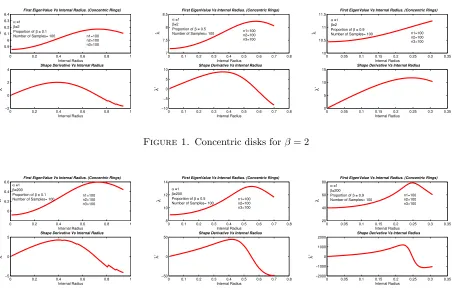
In the first of these experiments, we consider a domain which is a disk of unit radius and we assume the materialβ to be placed in an annular region having internal and external radiusr1 andr2 respectively within

a disk and the materialα, in the complement of this annulus within the unit disk. Letmbe the proportion of the total volume that the material β occupies so thatm= (r22−r12). We takeθto be the radial perturbation

which moves the annulus containingβ away from the centre while maintaining its area fixed.

In Figure 1 we plot the calculated numerical values of the first eigenvalue and the shape derivative as a function of the internal radius for the values α = 1, β = 2 and the proportions m = 0.1, 0.5, and 0.9 respectively. The shape derivative, in this case, is calculated using the simpler formula (2.1) after writing the

terms (σ|∇u|)2Siθ·nSiper(Si) as surface integrals Z

Si

(σ|∇u|)2Siθ·nSi dS. We do the same forα= 1,β = 200

in Figure 2.

0 0.2 0.4 0.6 0.8 1 5.9

6 6.1 6.2 6.3

6.4 First EigenValue Vs Internal Radius. (Concentric Rings)

Internal Radius

λ

α =1 β=2 Proportion of β = 0.1 Number of Samples= 100

0 0.2 0.4 0.6 0.8 1 −2

0 2

4 Shape Derivative Vs Internal Radius

Internal Radius λ ’ n1=100 n2=100 n3=100

0 0.1 0.2 0.3 0.4 0.5 0.6 0.7 0.8 7

7.5 8

Internal Radius

λ

0 0.1 0.2 0.3 0.4 0.5 0.6 0.7 0.8 −10

−5 0 5

0 0.05 0.1 0.15 0.2 0.25 0.3 0.35 10

10.5 11

Internal Radius

λ

0 0.05 0.1 0.15 0.2 0.25 0.3 0.35 0

5 10

Figure 1. Concentric disks forβ = 2

0 0.2 0.4 0.6 0.8 1 6

6.2 6.4

Internal Radius

λ

0 0.2 0.4 0.6 0.8 1 −5

0

0 0.1 0.2 0.3 0.4 0.5 0.6 0.7 0.8 8

10 12

14 First EigenValue Vs Internal Radius. (Concentric Rings)

Internal Radius

λ

0 0.1 0.2 0.3 0.4 0.5 0.6 0.7 0.8 −50

0

0 0.05 0.1 0.15 0.2 0.25 0.3 0.35 20

40 60

80 First EigenValue Vs Internal Radius. (Concentric Rings)

Internal Radius

λ

0 0.05 0.1 0.15 0.2 0.25 0.3 0.35 −2000

−1000 0 1000

Figure 2. Concentric disks forβ= 200

The numbersn1, n2 andn3 refer to the number of boundary nodes on the circles with radiusr1, r2 and 1

respectively.

We make the following observations.

In all the cases we see that the first eigenvalue is the smallest for r1 = 0 which corresponds to taking the

material β in the middle. The sign of the calculated shape derivative is positive in the intervals where λ1 is

seen to be increasing with respect tor1 and is negative whereλ1is seen to decrease withr1. As we know that

(10)

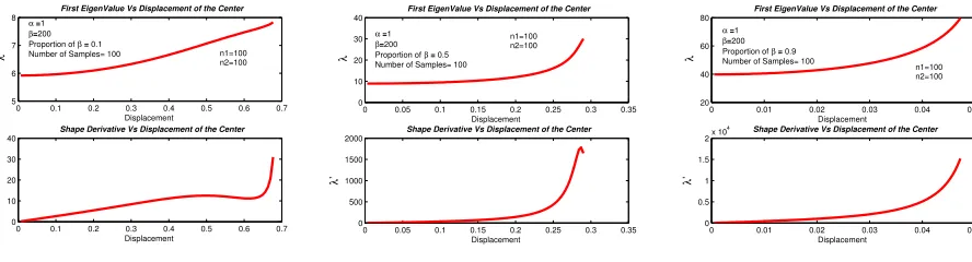
Although, we are guaranteed by the theorem of Alvino et. al. [2] that the minimization problem admits a radially symmetric minimizer it does not exclude the presence of other minimizers which do not have radial symmetry. With this in mind, we consider an experiment in a unit disk where the materialβ is put in a smaller disk whose area is a fraction m of the total area. The perturbation θ is the translation of the smaller disk outwards along the radial direction.

In Figure 3 we plot the first eigenvalue and the shape derivative as a function of the distancel between the centers of the two non-concentric disks takingα= 1,β= 2 and for the proportionsm= 0.1, 0.5, and 0.9. We do the same forα= 1,β= 200 in Figure 4.

0 0.1 0.2 0.3 0.4 0.5 0.6 0.7 5.9

6 6.1 6.2 6.3

6.4 First EigenValue Vs Displacement of the Center

Displacement

λ

0 0.1 0.2 0.3 0.4 0.5 0.6 0.7 0

1 2

3 Shape Derivative Vs Displacement of the Center

Displacement

λ

’

n1=100 n2=100

0 0.05 0.1 0.15 0.2 0.25 0.3 0.35 7

7.2 7.4

Displacement

λ

0 0.05 0.1 0.15 0.2 0.25 0.3 0.35 0

2 4 6

Displacement

λ

’

n1=100 n2=100

0 0.01 0.02 0.03 0.04 0.05 10.41

10.42 10.43

Displacement λ _α₌₁

β=2 Proportion of β = 0.9 Number of Samples= 100

0 0.01 0.02 0.03 0.04 0.05 −3

−2 −1

Displacement

λ

’

n1=100 n2=100

Figure 3. Non-concentric disks configurations forβ = 2

The numbers n1 and n2 refer to the number of nodes on the boundaries of the inner and outer disks,

respectively.

In general we see that we obtain smaller values for the eigenvalue when the inner disk is near the centre of the domain. Also, in general, we see that the sign of the shape derivative agrees with the behaviour shown the eigenvalue graph.

However, there are some cases where these do not seem to be the case. More precisely, we see when we take

α= 1 and β = 2 and m= 0.9 that the eigenvalue seems to be smaller when the disk is displaced. Actually, in carrying out the experiment for values of β of nearly the same order asα (for values not bigger than 2) a strange behaviour seems to arise as the proportion m approaches the value 0.755 and onwards. We try to explain this unexpected behaviour in the following way. One of the things to consider here is that the variation of the eigenvalues is of the order of 10−3 _{or less. In addition, the condition numbers of the matrices involved}

are very high (of the order 1028_{) due to the Dirichlet condition, and it becomes hard to distinguish the true}

variations in the calculated eigenvalues from the variation due to the numerical errors.

0 0.1 0.2 0.3 0.4 0.5 0.6 0.7 5

6 7

8 First EigenValue Vs Displacement of the Center

Displacement

λ

0 0.1 0.2 0.3 0.4 0.5 0.6 0.7 0

10 20 30

Displacement

λ

’

n1=100 n2=100

0 0.05 0.1 0.15 0.2 0.25 0.3 0.35 0

10 20 30

Displacement

λ

0 0.05 0.1 0.15 0.2 0.25 0.3 0.35 0

500 1000 1500

Displacement

λ

’

n1=100 n2=100

0 0.01 0.02 0.03 0.04 0.05 20

40 60

Displacement

λ

0 0.01 0.02 0.03 0.04 0.05 0

0.5 1 1.5 2x 10

Displacement

λ

’

n1=100 n2=100

(11)

We also see that the numerical values of shape derivative calculated using formula (1.11) behaves chaotically and show little correlation with the variations of the eigenvalue. Certainly we are inside a turbulent numerical region.

The numerical results were observed to normalize for values of the coefficientβ from 2.1 onwards.

3. _Conclusions

On the basis of the above numerical results we reach the conclusion that in domains like disks it may be better to place the material with higher conductivity in the middle in order to minimize the first eigenvalue. The shape derivative has been used in a limited way in this article to see the effect of some specific perturbations on certain configurations. It would be interesting to exploit the shape derivative calculated in this article in looking for directions of descent and in the development of algorithms which could help in automatic detection of the optimal distribution.

Acknowledgements: We would like to thank the referees of the article whose critical comments and helpful suggestions, in the form of pertinent references, have been important for a rigorous presentation of the results on shape derivative and for the rectification of some crucial errors. We would also like to thank Patricio Cumsille for useful discussions on the numerical computations involved.

References

[1] Afraites L, Dambrine M, Kateb D (2007) Shape methods for the transmission problem with a single measurement. Numerical Functional Analysis and Optimization 28(5) 519–551.

[2] Alvino A, Lions PL, Trombetti G (1989) Optimization problems with prescribed rearrangements. Nonlinear Analysis TMA 13(2): 185–220.

[3] Cox S, Lipton R (1996) Extremal eigenvalue problems for two-phase conductors. Arch. Rational Mech. Anal. 136: 101–117. [4] Conca C, Mahadevan R, Sanz L (2008) An extremal eigenvalue problem for a two-phase conductor in a ball, published online

inAppl. Math. Optim.

[5] Fern´andez Bonder JF, Groisman P, Rossi JD (2007), Optimization of the first Steklov eigenvalue in domains with holes: a

shape derivative approach. Ann. Mat. Pura. Appl. 186(2), 341–358.

[6] Gilbarg, Trudinger, Elliptic partial differential equations of second order, Springer.

[7] Henrot A (2006) Extremum Problems for Eigenvalues of Elliptic Operators. Birkha¨user.

[8] Henrot A, Pierre M (2005) Variation et Optimisation de Formes. Math´ematiques et Applications 48. Springer.

[9] Hettlich F, Rundell W (1998) The determination of a discontinuity from a single boundary measurement. Inverse Problems 14, 67–82.

[10] Kato T (1966) Perturbation Theory for Linear Operators, Classics in Mathematics. Springer-Verlag.

[11] Kre˘ın MG (1955) On certain problems on the maximum and minimum of characteristic values and on the Lyapunov zones of stability. AMS Translations Ser. 2(1): 163–187.

[12] Kre˘ın MG, Rutman MA (1950) Linear operators leaving invariant a cone in a Banach space. Amer. Math. Soc. Translation no. 26.

[13] Murat F, Tartar L (1997) Calculus of Variations and Homogenization (engl. transl. of original french article) in “Topics in the

Mathematical Modelling of Composite materials” Eds. A. Cherkaev and R.V. Kohn, PNLDE 31. Birkha¨auser.

[14] Simon J (1980) Differentiation with respect to the domain in boundary value problems. Numer. Funct. and Optimiz. 2(7-8), 649–687.

[15] Schiffer M (1946) Hadamard’s formula and variations of domain functions. Amer. J. Math. 68, 417–448.

[16] Shimakura N (1983) La premi`ere valeur propre du Laplacien pour le probl`eme de Dirichlet. J. Math. Pures. Appl. 62(2), 129–152.