A Hybrid Algorithm for a Two-Echelon Location- Routing Problem with Simultaneous Pickup and Delivery under Fuzzy Demand

(1)

59 International Journal of Transportation Engineering,

A Hybrid Algorithm for a Two-Echelon

Location-Routing Problem with

Simultaneous Pickup and

Delivery under Fuzzy Demand

Mohammadreza Ghatreh Samani 1, Seyyed-Mahdi Hosseini-Motlagh 2

Received: 09. 10. 2016 Accepted: 24. 04. 2017

Abstract

Location-Routing Problem (LRP) emerges as one of the hybrid optimization problems in distribution networks in which, total cost of the system would be reduced significantly by simultaneous optimization of locating a set of facilities among candidate locations and routing vehicles. In this paper, a mixed integer linear programming model is presented for a two-echelon location-routing problem with simultaneous pickup and delivery. In the investigated problem, one echelon of facilities, which is called the middle depot echelon, is positioned between central distribution centers and customers echelons. The number and capacity of middle depots and vehicles are considered to be limited. Besides, each network customer demands for both receiving a type of commodities and delivering another type to vehicles to be returned to the depot. In the literature of location routing problem, the majority of researches have been conducted in the deterministic conditions. However, we present a model in which data uncertainty is also taken into account and customers' demand is assumed to be a fuzzy parameter. We utilize a fuzzy programming approach to cope with uncertain demands. Moreover, a combined heuristic method based on simulated annealing (SA) algorithm and genetic algorithm (GA) is devised for solving the presented model. The results achieved from solving the problem in different sizes of numerical examples imply that the proposed hybrid algorithm outperforms other algorithms within reasonable length of time. The effectiveness of the proposed solution method is examined through a comprehensive numerical experiments. Finally, valuable insights are provided via conducting a number of sensitivity analyses.

Keywords: Location-routing problem; Two echelons; Fuzzy numbers; Credibility theory; Hybrid algorithm.

Corresponding author E-mail: [email protected]

1. PhD. Student, School of Industrial Engineering, Iran University of Science and Technology, Tehran, Iran

(2)

A Hybrid Algorithm for a Two-Echelon Location-Routing Problem with ….

1.

Introduction

Economic consideration is one of the most significant issues in business environment so enterprises have always been seeking the ways to reduce costs in different parts of organizations. The fact is that a great portion of these expenses belongs to logistics costs. Being a substantial part of any supply chains, distribution networks need to be appropriately designed to reduce costs and improve responsiveness of the chain. Increasing the efficiency of distribution systems can be considered as one of the primary goals of integrated logistics systems. Thus, optimization of logistics systems has become a critical problem in supply chain management in recent years. Integrated problems in distribution networks can be categorized into location-routing problems (LRP), location-inventory problems (LIP), inventory-routing problems (IRP), vehicle-routing problems (VRP), and so on [Majidi, Hosseini-Motlagh and Ignatius, 2017]. The location-routing problem (LRP) will convert to the vehicle-routing problem (VRP) if the location of facilities is predetermined. Location-routing problems are in the set of NP-hard problems, and solving each problem separately (i.e. once, the location-allocation problem and then routing problem) would result in sub-optimal solutions [Cheraghi, Hosseini-Motlagh and Ghatreh Samani, 2016].

Location and routing decisions are the two interdependent elements of a distribution network. Deciding on locating facilities without accounting for routing considerations may increase total network cost. [Laporte, 1987].

LRP is applicable in many fields such as food and beverage distribution, postal parcels

and pharmaceuticals deliveries and military applications.

In some cases, customers may have pickup and delivery demands at the same time. In such situations, the problem is called location-routing problem with simultaneous pickup and delivery (LRPSPD), which copes with determining the location of facilities and vehicles routes in such a way that both delivery and pickup demands for each customer are supposed to be simultaneously satisfied by vehicles to minimize total cost [Karaoglan et al. 2011]. Delivering car spare parts and collecting defective parts and so on can be considered as the applications of this problem.

(3)

Mohammadreza Ghatreh Samani , Seyyed-Mahdi Hosseini-Motlagh

61 International Journal of Transportation Engineering,

model is provided in Section 3. In Section 4, a fuzzy approach is developed to deal with the demand fuzziness. In Section 5, our heuristic method, which is the combination of meta-heuristic algorithms (i.e., simulated annealing and genetic algorithms) is presented. Section 6 provides several numerical examples to evaluate the effectiveness of the proposed method. Finally, concluding remarks and future works recommendations are given in Section 7.

2.

Literature Review

In this section, we first briefly review the related literature on the location-routing problem (LRP) and its derivatives (i.e. the location-routing problem with simultaneous pickup and delivery (LRPSPD) and the two-echelon location routing problem (2E-LRP)), then investigate the papers which have taken into account the data uncertainties.

The first study of location- routing problems refers to Webb [Webb, 1968]. The study was expanded by Watson-Gandy and Dohrn [Watson-Gandy and Dohrn, 1973], Nambiar, Gelders and Van Wassenhove [Nambiar, Gelders and Van Wassenhove, 1981] and Madsen [Madsen, 1983]. The location- routing problem could be classified based on different criteria. The first classification was provided by Min, Jayaraman and Srivastava [Min, Jayaraman and Srivastava, 1998]. Nagy and Salhi [Nagy and Salhi, 2007] classified this problem based on standard and non-standard structures and the type of objective functions. Recently, Prodhon and Prins [Prodhon and Prins, 2014] presented a classification of location-routing problems according to solution methods and modeling approaches.

LRPSPD, a branch of LRP, was firstly introduced by karaoglan et al. [karaoglan et

(4)

A Hybrid Algorithm for a Two-Echelon Location-Routing Problem with ….

2004] and the limitation on the capacity of vehicles as well as delivery constraints are taken into account. However, the capacity of facilities is considered to be unlimited. They tailored a two-phase algorithm in which the location of each facility is determined in the first phase, afterwards, vehicles routing is dealt with in the second phase. Ambrosino and Scutella [Ambrosino and Scutella, 2005] developed a two-echelon location-routing problem in which customers were visited in several clusters. A two-phase method was devised to solve their proposed model. In the first phase, customers' clustering, vehicles allocation to each cluster and the location of local facilities are determined by employing an integer programming model. Then, in the second phase, a travelling salesman problem (TSP) is solved for each cluster by using a branch-and-cut algorithm. Eventually, the solutions are improved through replacing local facilities with each other. Nikbakhsh and Zegordi [Nikbakhsh and Zegordi, 2010] worked on a model for the two-echelon capacitated location-routing problem, in which the capacity of both vehicles and facilities was assumed to be limited. They regarded constraints on maximum tour length for vehicles and applied a heuristic method along with a meta-heuristic algorithm based on simulated annealing (SA) to solve the problem. Moreover, the corresponding results were evaluated by solving the problem in different sizes.

Although the related papers on the subject of LRP have been mostly considered in deterministic conditions, inadequate knowledge of uncertain parameters such as demand, travel time and so on has made the researchers consider uncertainty conditions in their works to have a better perception of reality. In this regard, a location-routing

problem with time windows (LRPTW) was presented by Zarandi et al. [Zarandi et al., 2013]. They considered travel time as a fuzzy parameter and employed simulated annealing (SA) to solve the model, then compared the respective results with those existing in the literature. Golozari, Jafari, and Amiri [Golozari, Jafari, and Amiri, 2013] worked on a routing problem while considering the constraint on maximum route length. In the concerned problem, customers' demand and travel time as well as service time were regarded to be fuzzy parameters. They used simulated annealing (SA) algorithm to solve the presented model. Nadizadeh and Hosseini Nasab [Nadizadeh and Hosseini Nasab, 2014] proposed a model for the location-routing problem under fuzzy demand over a multi-period planning horizon, and devised a clustering approach to solve the proposed model.

Recently, Riquelme-Rodríguez, Gamache and Langevin [Riquelme-Rodríguez, Gamache, and Langevin, 2016] addressed the first method for a periodic capacitated location arc routing problem for suppressing dust in hauling roads. They proposed two methods for finding the initial location of water depots in the road and then compared their performance with the aim of minimizing penalty costs arising from the lack of humidity in roads as well as routing costs. Afterwards, the initial location of water depots and the initial vehicle routing were modified by applying an exchange algorithm and an adaptive large neighborhood search algorithm, respectively.

(5)

Mohammadreza Ghatreh Samani , Seyyed-Mahdi Hosseini-Motlagh

demand amounts as well as volume of products were considered to be tainted with uncertainty. Minimizing the cost of used vehicles, fuel consumption along with the shortage of products are the two objectives of the problem. They applied the ε-constraint method to solve the proposed bi-objective model and devised a fuzzy programming approach to deal with the uncertainty. Hiassat, Diabat and Rahwan [Hiassat, Diabat and Rahwan, 2017] proposed a mixed integer programming model for a location-inventory-routing problem for perishable products. Their research aimed to determine the location and required number of depots, the level of inventory at each retailer, and the travelling routes. They developed a Genetic Algorithm approach to solve the under-investigated problem and obtained near-optimal solutions in reasonable length of time. A novel approach for location routing problem was presented by Schiffer and Walther [Schiffer and Walther, 2017] while considering strategic planning for electric logistics fleets. The approach considers the decisions of charging station siting and vehicle routing simultaneously to illustrate the significance of jointly consideration of siting and routing decisions. Applying the proposed approach, they minimized total costs, distance, and the number of vehicles and charging stations concurrently. In an effort, Nikkhah Qamsari, Hosseini-Motlagh and Jokar [Nikkhah Qamsari, Hosseini-Motlagh and Jokar, 2017] developed a two phase hybrid heuristic approach to solve the multi-depot multi-vehicle routing problem while accounting for inventory constraints. Their concerned model aimed to minimize total cost including inventory holding cost at distribution centers and the customers' side as well as transportation costs. They applied a

variable neighborhood search algorithm to modify the initial solution obtained in construction phase. They illustrated the capability of their proposed algorithm to find near-optimal solutions within reasonable computing time.

To the best of our knowledge, the majority of studies have addressed the two-echelon location-routing problem in deterministic condition and a study on this subject while considering uncertainty conditions is non-existent. To fill this gap, our research is differentiated from the ones existing in the literature of LRP by considering the following contributions:

 A mixed integer linear programming model for a two-echelon location- routing problem with simultaneous pickup and delivery under uncertainty is proposed.

 The uncertainty in customers' demand is accounted for in the form of fuzzy numbers which is handled by applying a fuzzy credibility programming approach.

 The proposed model is solved by means of a hybrid solution approach which is the combination of genetic and simulated annealing algorithms.

3.

Problem description

(6)

A Hybrid Algorithm for a Two-Echelon Location-Routing Problem with ….

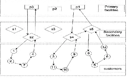
storing, loading and unloading goods. The concerned 2E - LRPSPD can be schematically depicted in Figure 1. In this research, we seek to optimize the number of open facilities along with routing between established secondary and central facilities as well as routing between customers and secondary facilities with the aim of customers' demand satisfaction and minimizing the network total cost including establishment cost, travelling cost and vehicles fixed cost. In the concerned network, travelling route starts from a main depot and ends at the same depot. Each vehicle belongs to one route and is in charge of delivering goods from main depot to the secondary depot and from secondary depot to customers such that each customer is visited exactly once and the customers' demands do not exceed the capacity of the vehicle, and picking up goods from customers to return to the same depot.

Figure 1.The considered two-echelon location-routing problem

3.1

Mathematical Formulation in

Deterministic Mood

Consider graph 𝐺 = (𝑉, 𝐸) in which 𝑉 represents the set of network nodes which includes 𝑉_𝑂, the set of central depots, VR, the set of middle depots and 𝑉𝐶, the set of customers. In this graph, 𝑉1 and 𝑉2 indicates

the nodes of the first and second echelons, respectively, such that (𝑉1= 𝑉𝑂∪ 𝑉𝑅) and (𝑉₂= 𝑉_𝑅∪ 𝑉_𝐶). The set of total existing arcs of the graph (E) includes undirected arcs connecting central distribution centers to middle ones, middle distribution centers to customers and customers to each other. The connecting arcs must satisfy the following triangular inequality (𝑑𝑖𝑗 ≤ 𝑑𝑖𝑘+ 𝑑𝑘𝑗). Set K includes vehicles which are used between middle distribution centers and customers in the second echelon. The aforementioned problem is studied under the following constraints:

 Each vehicle travels a route while starting from a specific depot and finishing in the same depot.

 Each route can provide services for only one vehicle.

 Each customer is allowed to be served by only one vehicle.

 Customers' pickup and delivery demands are satisfied simultaneously and do not exceed the capacity of vehicles.

 Total demands from customers allocated to a depot do not exceed the depot capacity.

 Total demands in a route do not exceed the capacity of vehicle assigned to that route.

(7)

Mohammadreza Ghatreh Samani , Seyyed-Mahdi Hosseini-Motlagh

Model sets, parameters and decision variable

s

3.1.1.

Sets

I The set of customers

O The set of central depots

R The set of candidate middle depots

K The set of vehicles

3.1.2.

Technical parameters

CDO The capacity of each central depot RDR The capacity of each middle depot

di The amount of each customer’s delivery demand pi The amount of each customer’s pickup demand CV The capacity of each vehicle

3.1.3.

Cost parameters

FR Establishment fixed cost of each middle depot

GOR Travel cost between a pair of central and middle depots Hij Travel cost from customer i to j

FCk Fixed cost of each vehicle

3.1.4.

Decision variables

3.1.4 Objective Function

𝑀𝑖𝑛 ∑ ∑ 𝐻𝑖𝑗𝑦𝑖𝑗+ ∑ ∑ 𝐺𝑂𝑅𝑥𝑂𝑅 𝑅∈𝑁_𝑅 𝑂∈𝑉_𝑂 𝑗∈𝑉₂

𝑖∈𝑉₂

+ ∑ 𝐹𝑅𝑤𝑅+ 𝑅∈𝑉_𝑅

∑ ∑ 𝐹𝐶𝑘𝑝𝑖𝑅 𝑅∈𝑉_𝑅 𝑖∈𝑉₂

( 1 )

3.1.5 Model Constraints

∑ 𝑥𝑂𝑅≤ 𝐶𝐷𝑂 𝑅∈𝑉_𝑅

∀O ∈ 𝑉𝑂 )2(

∑ 𝑥𝑂𝑅≤ 𝑅𝐷𝑅∗ 𝑂∈𝑉_𝑂

𝑂𝑅 ∀R ∈ 𝑉𝑅 )3(

∑ 𝑥𝑂𝑅≥ ∑ 𝑑𝑖∗ 𝑖∈𝑉₂ 𝑂∈𝑉_𝑂

𝑝𝑖𝑅 ∀R ∈ 𝑉𝑅 )4(

∑ 𝑦𝑖𝑗 𝑗∈𝑉₂

= 1 ∀i ∈ 𝑉𝐶 )5(

𝐱𝐎𝐑 _{The amount of commodity transported from central depot}_O_{to middle depot R.} (∀R ∈ VR, ∀O ∈

(8)

A Hybrid Algorithm for a Two-Echelon Location-Routing Problem with ….

∑ 𝑦𝑗𝑖= ∑ 𝑦𝑖𝑗 𝑗∈𝑁2 𝑗∈𝑉2

∀i ∈ 𝑉2 )6(

∑ 𝑝𝑖𝑅= 1 𝑅∈𝑉𝑅

∀i ∈ 𝑉𝐶 )7(

∑ 𝑑𝑖∗ 𝑝𝑖𝑅≤ 𝑅𝐷𝑅∗ 𝑂𝑅 𝑖∈𝑉₂

∀R ∈ 𝑉𝑅 )8(

∑ 𝑝𝑖∗ 𝑝𝑖𝑅≤ 𝑅𝐷𝑅∗ 𝑂𝑅 𝑖∈𝑉₂

∀R ∈ 𝑉𝑅 )9(

𝑍𝑗− 𝑍𝑖+ 𝐶𝑉 ∗ 𝑦𝑖𝑗+ (𝐶𝑉 − 𝑑𝑖− 𝑑𝑗)𝑦𝑗𝑖+ 𝑑𝑖≤ 𝐶𝑉

∀i, j ∈ 𝑉𝑐, 𝑖 ≠ 𝑗 )10(

𝑊𝑗− 𝑊𝑖+ 𝐶𝑉 ∗ 𝑦𝑖𝑗+ (𝐶𝑉 − 𝑝𝑖− 𝑝𝑗)𝑦𝑗𝑖+ 𝑝𝑖≤ 𝐶𝑉

∀i, j ∈ 𝑉𝑐, 𝑖 ≠ 𝑗 )11(

𝑍𝑖+ 𝑊𝑖− 𝑑𝑖≤ 𝐶𝑉 ∀i ∈ 𝑉𝐶 )12(

𝑑𝑖+ ∑ 𝑑𝑗𝑦𝑖𝑗≤ 𝑍𝑖 𝑗∈𝑉_𝐶,𝑗≠𝑖

∀i ∈ 𝑉𝐶 )13(

𝑝𝑖+ ∑ 𝑝𝑗𝑦𝑖𝑗≤ 𝑊𝑖 𝑗∈𝑉𝐶,𝑗≠𝑖

∀i ∈ 𝑉𝐶 )14(

𝑍𝑖+ ( 𝐶𝑉 − 𝑑𝑖)( ∑ 𝑦𝑖𝑅 𝑅∈𝑉_𝑅

) ≤ 𝐶𝑉 ∀i ∈ 𝑉𝐶 )15(

𝑊𝑖+ ( 𝐶𝑉 − 𝑝𝑖)( ∑ 𝑦𝑅𝑖 𝑅∈𝑉_𝑅

) ≤ 𝐶𝑉 ∀i ∈ 𝑉𝐶 )16(

𝑦𝑖𝑅≤ 𝑝𝑖𝑅 ∀i ∈ 𝑉𝐶, ∀𝑅 ∈ 𝑉𝑅 )17(

𝑦𝑅𝑖≤ 𝑝𝑖𝑅 ∀i ∈ 𝑉𝐶, ∀𝑅 ∈ 𝑉𝑅 )18(

𝑦𝑖𝑗+ 𝑝𝑖𝑅+ ∑ 𝑝𝑗𝑚≤ 2 𝑚∈𝑉𝑅,𝑚≠𝑅

∀i, j ∈ 𝑉𝑐, 𝑖 ≠ 𝑗 ,∀𝑅 ∈ 𝑉𝑅 )19(

𝑦𝑖𝑗∈ {0,1} ∀i, j ∈ 𝑉2 )20(

𝑥𝑂𝑅 ≥ 0 ∀O ∈ 𝑉𝑂, ∀R ∈ 𝑉𝑅 )21(

𝑝𝑖𝑅∈ {0,1} ∀i ∈ 𝑉𝐶 )22(

𝑂𝑅∈ {0,1} ∀𝑅 ∈ 𝑉𝑅 )23(

𝑍𝑖≥ 0 ∀i ∈ 𝑉2 )24(

(9)

Mohammadreza Ghatreh Samani , Seyyed-Mahdi Hosseini-Motlagh

The objective function (1) aims to minimize the total cost of the network consisting of travel costs in the first and second distribution levels, establishment fixed cost of middle depots, and vehicles fixed costs. Constraint (2) shows the capacity limitation of central depots. In other words, the amount of goods stored in a central depot and distributed to a middle depot does not exceed the capacity of the central depot. The limited capacity of middle depots is represented by constraint (3). Better to say, the amount of goods received by a middle depot does not exceed the capacity of the depot. Constraint (4) is the inflow and outflow conservation constraint for middle depots. It guarantees that the amount of goods received by each middle depot is equal to the amount of goods dispatched from the depot. In other words, middle depots act as a bridge between central depots and customers. Each customer is allowed to be visited exactly once by any vehicles. This is guaranteed by constraint (5). Constraint (6) denotes the inflow and outflow conservation constraint for each customer. Indeed, this constraint states that each customer is once visited and delivered the goods and is left while picking up the required goods. Constraint (7) ensures that each customer can be assigned to only one middle depot. Constraints (8) indicates that total demand which is delivered from each middle depot to customer does not exceed the capacity of the middle depot. Constraint (9) ensures that total pickup demand from customers to each middle depot does not exceed the capacity of the depot. Constraints (10) and (11) determine delivery and pickup flows in each arc, considering the capacity of vehicles, respectively. In other words, total delivery demand to each customer and total pickup demand from each customer do not exceed the capacity of the vehicle. Constraint (12) shows the maximum capacity of

each vehicle. Constraints (13) and (15) define lower bound and upper bound of total delivery demand variable. Similarly, constraints (14) and (16) denote lower bound and upper bound of total pickup demand variable. Constraints (17)-(19) denote sub-tour elimination constraints. Better to say, these constraints prevent undesirable tours in which some customers are neglected to be visited or vehicles, starting from a specific depot, do not return to the same depot at the end of the service. Constraints (20)-(25) specify the type of decision variables.

4.

Fuzzy Programming Approach

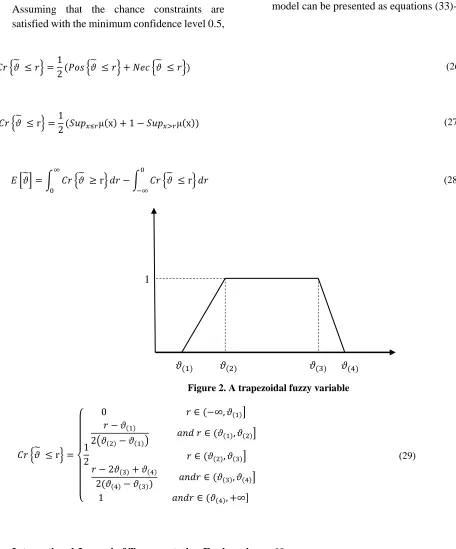
In this section, we devise a fuzzy programming approach based on the credibility theory to cope with the customers' fuzzy demands. The problem is handled by applying a credibility-based chance constrained programming method as an efficient fuzzy approach because it enables the decision maker to satisfy the chance constraints at least at a minimum confidence level 𝛼, and can be applied for both triangular and trapezoidal fuzzy numbers [Cheraghi, Hosseini-Motlagh, 2016]. Let 𝜗̃ be a fuzzy variable with membership function 𝜇(𝑥) and 𝑟 be a real number. The credibility measure can be formulated as follows. (Equation 26) [Liu and Liu, 2002] Since the 𝑃𝑜𝑠 {𝜗̃ ≤ r} =

𝑆𝑢𝑝𝑥≤𝑟μ(x) and 𝑁𝑒𝑐 {𝜗̃ ≤ r} = 1 − 𝑆𝑢𝑝𝑥>𝑟μ(x)

the relationship (26) can be substitute by the following equation. Thus, the expected value of 𝜗̃ based on credibility measure is represented by equation (28). If ϑ̃ be a trapezoidal fuzzy number, as shown in Figure 2, such thatϑ̃ =

(ϑ(1), ϑ(2), ϑ(3), ϑ(4)), the expected value of ̃ϑ will

be equal to(ϑ(1)+ ϑ(2)+ ϑ(3)+ ϑ(4))/4 , and the

(10)

A Hybrid Algorithm for a Two-Echelon Location-Routing Problem with ….

credibility measure will be equivalent by equations (30). [Zhu and Zhang, 2009]

4.1 The Equivalent Auxiliary Crisp

Model

Assuming that the chance constraints are satisfied with the minimum confidence level 0.5,

or better to say, 𝛼 > 0.5, the proposed model can be converted to the equivalent crisp one using the relationships (31) and (32). However, the rest of the elements will remain unchanged. According to the above descriptions, the equivalent crisp model can be presented as equations (33)-(42).

( 26 )

𝐶𝑟 {𝜗̃ ≤ 𝑟} =1

2(𝑃𝑜𝑠 {𝜗̃ ≤ 𝑟} + 𝑁𝑒𝑐 {𝜗̃ ≤ 𝑟})

( 27 )

𝐶𝑟 {𝜗̃ ≤ r} =1

2(𝑆𝑢𝑝𝑥≤𝑟μ(x) + 1 − 𝑆𝑢𝑝𝑥>𝑟μ(x))

( 28 )

𝐸 [𝜗̃] = ∫ 𝐶𝑟 {𝜗̃ ≥ r}∞ 0

𝑑𝑟 − ∫ 𝐶𝑟 {𝜗̃ ≤ r}0 −∞

𝑑𝑟

Figure 2. A trapezoidal fuzzy variable

( 29 )

𝐶𝑟 {𝜗̃ ≤ r} =

{ 1 2

0 𝑟 ∈ (−∞, 𝜗(1)] 𝑟 − 𝜗(1)

2(𝜗(2)− 𝜗(1))

𝑎𝑛𝑑 𝑟 ∈ (𝜗(1), 𝜗(2)]

𝑟 ∈ (𝜗(2), 𝜗(3)] 𝑟 − 2𝜗(3)+ 𝜗(4)

2(𝜗(4)− 𝜗(3)) 𝑎𝑛𝑑𝑟 ∈ (𝜗(3), 𝜗(4)] 1 𝑎𝑛𝑑𝑟 ∈ (𝜗(4), +∞]

1

(11)

( 30 )

𝐶𝑟 {𝜗̃ ≥ r} =

{ 1 2

1 𝑟 ∈ (−∞, 𝜗(1)] 2𝜗(2)− 𝜗(1)− 𝑟

2(𝜗(2)− 𝜗(1)) 𝑎𝑛𝑑𝑟 ∈ (𝜗(1), 𝜗(2)] 𝑟 ∈ (𝜗(2), 𝜗(3)]

𝜗(4)− 𝑟

2(𝜗(4)− 𝜗(3)) 𝑎𝑛𝑑 𝑟 ∈ (𝜗(3), 𝜗(4)] 0 𝑎𝑛𝑑𝑟 ∈ (𝜗(4), +∞]

( 31 )

𝐶𝑟 {𝜗̃ ≤ r} ≥α⇔ 𝑟 ≥ (2 − 2𝛼)𝜗(3)+ (2𝛼 − 1)𝜗(4)

( 32 )

𝐶𝑟 {𝜗̃ ≥ r} ≥α⇔ 𝑟 ≥ (2𝛼 − 1)𝜗(1)+ (2 − 2𝛼)𝜗(2)

𝒅𝒊,𝒇(𝒏)𝒔 The amount of each customer's delivery demand under each scenario

𝒑𝒊,𝒇(𝒏)𝒔 The amount of each customer's pickup demand under each scenario

∑ 𝑥𝑂𝑅𝑆 ≥ ∑ ((2 − 2α) ∗ di,𝑓(3)S + (2α − 1) ∗ di,𝑓(4)S ) ∗ 𝑝𝑖𝑅𝑆 𝑖∈𝑉2

𝑂∈𝑉𝑂

∀R ∈ 𝑉𝑅, ∀𝑠 (33)

∑ ((2 − 2α) ∗ di,𝑓(3)S + (2α − 1) ∗ di,𝑓(4)S ) ∗ 𝑝𝑖𝑅𝑆 ≤ 𝑅𝐷𝑅∗ 𝑂𝑅 𝑖∈𝑉2

∀R ∈ 𝑉𝑅, ∀𝑠 (34)

∑ ((2 − 2α) ∗ pi,𝑓(3)S + (2α − 1) ∗ pi,𝑓(4)S ) ∗ 𝑝𝑖𝑅𝑆 ≤ 𝑅𝐷𝑅∗ 𝑂𝑅 𝑖∈𝑉₂

∀R ∈ 𝑉𝑅, ∀𝑠 (35)

𝑍𝑗𝑆− 𝑍𝑖𝑆+ 𝐶𝑉 ∗ 𝑦𝑖𝑗𝑆

+ (𝐶𝑉 − ((2 − 2α) ∗ di,𝑓(3)S + (2α − 1) ∗ di,𝑓(4)S )

− ((2 − 2α) ∗ dj,𝑓(3)S + (2α − 1) ∗ dj,𝑓(4)S )) 𝑦𝑗𝑖𝑆 + ((2 − 2α) ∗ di,𝑓(3)S + (2α − 1) ∗ di,𝑓(4)S ) ≤ 𝐶𝑉

∀i, j ∈ 𝑉𝑐, 𝑖 ≠ 𝑗, ∀𝑠

(12)

A Hybrid Algorithm for a Two-Echelon Location-Routing Problem with ….

𝑊𝑗𝑆− 𝑊𝑖𝑆+ 𝐶𝑉 ∗ 𝑦𝑖𝑗𝑆

+ (𝐶𝑉 − ((2 − 2α) ∗ pi,𝑓(3)S + (2α − 1) ∗ pi,𝑓(4)S )

− ((2 − 2α) ∗ pj,𝑓(3)S + (2α − 1) ∗ pj,𝑓(4)S )) 𝑦𝑗𝑖𝑆

+ ((2 − 2α) ∗ pi,𝑓(3)S + (2α − 1) ∗ pi,𝑓(4)S ) ≤ 𝐶𝑉

∀i, j ∈ 𝑉𝑐, 𝑖

≠ 𝑗, ∀𝑠 (37)

𝑍𝑖𝑆+ 𝑊𝑖𝑆− ((2 − 2α) ∗ dSi,𝑓(3)+ (2α − 1) ∗ di,𝑓(4)S ) ≤ 𝐶𝑉 ∀i ∈ 𝑉𝐶, ∀𝑠 (38)

((2 − 2α) ∗ di,𝑓(3)S + (2α − 1) ∗ di,𝑓(4)S )

+ ∑ ((2 − 2α) ∗ dj,𝑓(3)S + (2α − 1) ∗ dj,𝑓(4)S ) 𝑦𝑖𝑗𝑆 ≤ 𝑗∈𝑉_𝐶,𝑗≠𝑖

𝑍𝑖𝑆

∀i ∈ 𝑉𝐶, ∀𝑠 (39)

((2 − 2α) ∗ pi,𝑓(3)S + (2α − 1) ∗ pi,𝑓(4)S )

+ ∑ ((2 − 2α) ∗ pj,𝑓(3)S + (2α − 1) ∗ pj,𝑓(4)S ) ∗ 𝑦𝑖𝑗𝑆 ≤ 𝑊𝑖𝑆 𝑗∈𝑉_𝐶,𝑗≠𝑖

∀i ∈ 𝑉𝐶, ∀𝑠 (40)

𝑍𝑖𝑆+ ( 𝐶𝑉 − ((2 − 2α) ∗ di,𝑓(3)S + (2α − 1) ∗ di,𝑓(4)S ))( ∑ 𝑦𝑖𝑅𝑆 𝑅∈𝑉_𝑅

) ≤ 𝐶𝑉 ∀i ∈ 𝑉𝐶, ∀𝑠 (41)

𝑊𝑖𝑆+ ( 𝐶𝑉 − ((2 − 2α) ∗ pi,𝑓(3)S + (2α − 1) ∗ pi,𝑓(4)S ))( ∑ 𝑦𝑅𝑖𝑆 𝑅∈𝑉_𝑅

) ≤ 𝐶𝑉 ∀i ∈ 𝑉𝐶, ∀𝑠 (42)

5.

Solution Methods

5.1 Genetic Algorithm (GA)

Genetic algorithm, presented by Holland [Holland, 1975], is a random research technique based on natural mechanism, combination and mutation genetic rules. Genetic algorithm starts with an initial set of random solutions which are named initial populations. Each population member is called a chromosome, which shows a solution for the problem and evolves during iterative periods. The population changes in each period and creates a new generation which is nearer to optimal solution than the previous generation.

5.2

Simulated

Annealing

(SA)

Algorithm

(13)

Mohammadreza Ghatreh Samani , Seyyed-Mahdi Hosseini-Motlagh

solid body and solution costs are equivalent to different energy levels (E).

5.3 The Proposed Algorithm

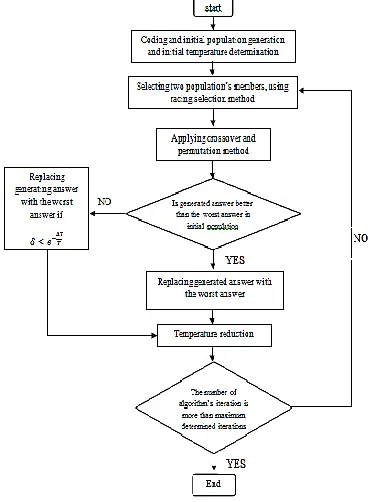
In this research, a hybrid algorithm which is the combination of dynamic programming, genetic and simulated annealing algorithms is presented. The visual representation of the proposed hybrid algorithm can be shown in Figure 3.

Figure 3. Flow chart of the GA-SA for the concerned problem

5.4 Chromosome Displays Mode

In this part, we intend to display a feasible solution mode for the problem. In the following, a chromosome is shown for 3 intermediate depots under specific scenarios. As can be seen, the designed chromosome for this problem is represented in 3 parts.

5.4.1 Part 1

The first part indicates a state in which whether an intermediate depot is activated or

not. It is equal to 1 if the intermediate depot is activated and 0, otherwise. The matrix dimension is 1*R, in which R represents the number of intermediate depots.

5.4.2 Part 2

The dimension of the matrix belonging to the second part is 1*l, in which l represents the number of customers. Digit 1 indicates intermediate depot activation and digit 0 indicates intermediate depot inactivation. A depot is chosen for each customer among the activated depots (in this example intermediate depots 1 and 2 are activated).

5.4.3 Part 3

Chromosome's third part shows how to meet the demand of customers allocated to each intermediate depot. In other words, it expresses the route and the pattern of customers' serving. Considering the first row of the previous part of chromosome, customers 1, 2,3,5,6 and 7 are allocated to intermediate depot 1 based on the dynamic algorithm. So the first row of chromosome’s third part, which is relevant to the first intermediate depot, shows that the sequence of customers' serving is that a vehicle moves from intermediate depot 1 to customer 3 and subsequently to customers5,6,2,7 and 1, then returns to the same depot.

(14)

A Hybrid Algorithm for a Two-Echelon Location-Routing Problem with ….

The third intermediate depot is not activated, thus no customer is allocated to this depot.

To determine the optimal vehicles routes, we have employed dynamic programming, which improves the objective function value of initial generated solutions in comparison with random mode.

5.5 Finding the initial solution

Held and Krap [Held and Krap, 1962] proposed a dynamic programming approach to solve the sequential problems. Their solutions can be applied for scheduling problems, the traveling sales man (TSP) problem and assembly line balancing problems. Their proposed solution method is computationally efficient in specifying limited range. In addition, the approximate solutions might be achieved by solving the sequences of small sub-problems which have the same structures.

5.6 Fitness Function

Fitness function is a criterion to measure the quality of solution obtained by the chromosome. Each chromosome’s fitness is computed based on objective function value in the mathematical model, the activation cost of each intermediate depot and customers' serving costs.

5.7 Choosing parents

In this phase, two members of the generated population are selected as parents, then a crossover operator is applied. The considered selection method in the presented algorithm is called "racing method" in which P

members of the population are randomly selected. Then, the members, which have the best objective function values among these P

members, are considered as parents.

5.8 Genetic operators

After selecting parents, the offspring must be generated by applying appropriate operators.

5.9 Crossover operators

In this paper, a crossover operator is used, in which we generate random numbers for each chromosome's first and second parts, and then, the crossover operator is applied to generate new offspring. Note that the first row of chromosome’s second part (i.e. customers' allocation to intermediate depots) is reliant on chromosome’s first part, this row is randomly generated based on initial solutions. On the other hand, chromosome's third part or routing part, completely depends on the first and the second parts. Accordingly, after applying crossover operator on the first and the second parts, we generate the third part based on initial generated solution. The following Example describes the crossover operator.

Assume that the first and the second parts of parents' chromosomes for a specific scenario is as follows:

(15)

Mohammadreza Ghatreh Samani , Seyyed-Mahdi Hosseini-Motlagh

Crossover operator is applied for parents under each scenario, separately.

5.10 Permutation Operator

In this phase, Firstly one population member is randomly selected, then a new solution is generated by creating a small change in the selected member. Permutation operator may increase the dispersion of solutions thus the searching process. In the presented algorithm, permutation operator is applied on chromosome’s second part. The first part is the first row of chromosome’s second part or customer’s allocation to intermediate depots. The second part of permutation is applied on chromosome’s third part or routing part. Two types of permutation operators are used in the presented algorithm as follows:

5.10.1 Swap

In this method, two genes of the chromosome are selected and their places are changed with each other. It is assumed that represented chromosome in chromosome display part for a specific scenario is selected randomly for permutation operator.

Let the second and the fourth parts be selected.

After changing the digits of places two and three, customers' allocation part is changed as follows:

The same must be done for routing part as well.

5.10.2 Reversion

In this permutation operator, two genes are selected from the chromosome, then digits between two genes are re-arranged. In that example, points 1 and 3 of intermediate depot 2 of the chromosome’s third part are selected for the reversion permutation operator.

The above part changes as follows, while applying permutation operator:

In this way, it can be seen that permutation and crossover are the two complementary operators. In other words, crossover operator impacts on two parts of a chromosome and permutation operator has influence on the other parts. It must be noted that in each permutation, selecting the permutation method occurs randomly with equal probability. Permutation operator is implemented for each scenario separately.

5.10.2.1 Comparing Generated Solution with the Worst Member of Population

After applying permutation and crossover operators and generating new solutions, each solution is compared with the worst member of initial population and would be replaced with the worst solution if it is better; otherwise, new solution is replaced with the worst existing solution in the population with the following probability:

δ≤ e−(∆ET ) (58)

∆E =newsol. Cost − sol. Cost sol. Cost

(16)

T=alpha*T (60)

in which new sol. cost represents objective function value of the new generated solution and T is the temperature in that iteration which reduces as equation (60), and finally 𝛿 is a uniformly generated number between 0 and 1.

5.11 Stop Criterion

As shown in Table 1, the appropriate values of the algorithm parameters are obtained by several runes of the algorithm using trial and error method. It is worth nothing that the considered criterion to stop algorithm is maximum number of generations.

Table 1.The algorithm parameters

6.

Numerical experiments

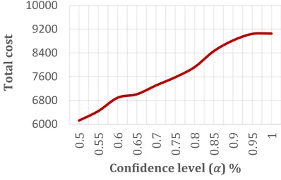
To validate the proposed model and its solution approach, several numerical examples are investigated. The problem is solved under different 𝛼 values. An analysis could be performed to examine the impact of changing service level on the network total cost. As can be observed in Figure.4, the increased value of α leads to the increased number of vehicles, which in turn increases the network total cost. However, we cannot see any changes in the number of vehicles when α grows from 0.6 to 0.65 and from 0.95 to 1. Therefore, the increase of objective function value could be possible due to the increase of transportation cost imposed by the increased value of service level to satisfy the fuzzy demands. Accordingly, decision makers (DM) need to determine conditions in which the demands are satisfied at higher confidence level α, however, it imposes

higher costs on the network. Indeed, the DM has to make a tradeoff between cost and demand satisfaction to decide on an appropriate confidence level.

Figure 4. The impact of different 𝜶 values on network total cost

In the following, we solve the problem in three different sizes (i.e. small size with 20 customers and 5 middle depots, medium size with 50 customers and 5 middle depots and large size with 100 customers and 5 and 10 middle depots) and their results are reported in Tables 2-4 using different methods including genetic algorithm, hybrid genetic algorithm, simulated annealing and also the combination of genetic and simulated annealing algorithms and dynamic programming approach.

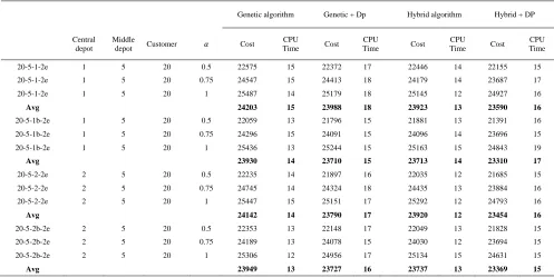
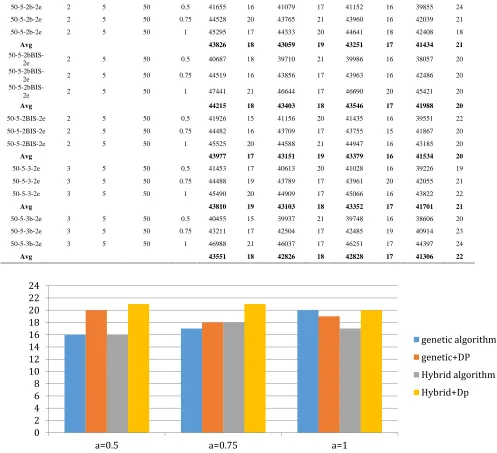
The results imply that, on average, the combination of genetic and simulated annealing algorithms often has better performance in comparison with genetic algorithm in terms of network costs and CPU time. The proposed method which is the combination of genetic and simulated annealing algorithms and using dynamic programming to find initial solution, outperforms the three other methods in terms of network total cost, however, it increases CPU time a bit more. Therefore, a general observation confirms high efficiency of the proposed algorithm for the problem in different sizes.

The analyses of diagrams in Figure 5 indicate that computational time of the proposed

6000 6800 7600 8400 9200 10000

0.

5

0.55 0.

6

0.65 0.

7

0.75 0.

8

0.85 0.

9

0.95

1

Total

co

st

(17)

hybrid algorithm increases as the service level 𝜶 is enhanced from 0.5 to 1, while genetic algorithm has a better performance in this situation since it reduces the computational time on average. On the other hand, the results, which is shown in Figure 6, represent the domination of the proposed hybrid algorithm performance over the three other methods in terms of network costs. As can be observed, genetic algorithm has the weakest performance among the algorithms. Moreover, although the combination of genetic algorithm and dynamic programming approach increases the computational time, it can result in the decreased network costs. As can be seen in Figure 7, in the problem of

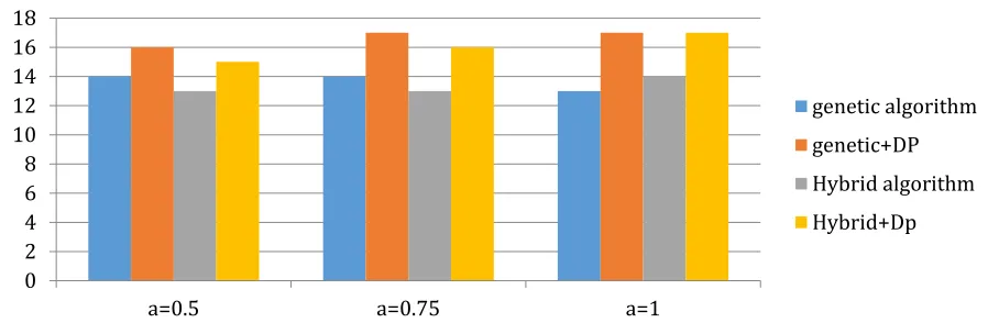
medium size, the computational time for solving the problem by genetic algorithm increases from 16 to 20 minutes as the value of 𝛼 grows from 0.5 to 1, while the CPU time for the proposed hybrid algorithm decreases from 21 minutes at confidence level 0.5 and reaches 20 minutes at 𝛼 = 1. Other two methods do not show specific patterns in computational length of time. Figure 8 depicts the efficiency of the proposed hybrid algorithm among other three methods in which the lowest level of cost is achieved by applying this algorithm. Furthermore, genetic algorithm has the worst performance and other two algorithms perform quite similarly in terms of network costs.

Table 2. Detailed results for Prodhon's instances in small size

Genetic algorithm Genetic + Dp Hybrid algorithm Hybrid + DP Central

depot

Middle

depot Customer 𝛼 Cost

CPU

Time Cost

CPU

Time Cost

CPU

Time Cost

CPU Time

20-5-1-2e 1 5 20 0.5 22575 15 22372 17 22446 14 22155 15

20-5-1-2e 1 5 20 0.75 24547 15 24413 18 24179 14 23687 17

20-5-1-2e 1 5 20 1 25487 14 25179 18 25145 12 24927 16

Avg 24203 15 23988 18 23923 13 23590 16

20-5-1b-2e 1 5 20 0.5 22059 13 21796 15 21881 13 21391 16

20-5-1b-2e 1 5 20 0.75 24296 15 24091 15 24096 14 23696 15

20-5-1b-2e 1 5 20 1 25436 13 25244 15 25163 15 24843 19

Avg 23930 14 23710 15 23713 14 23310 17

20-5-2-2e 2 5 20 0.5 22235 14 21897 16 22035 12 21685 15

20-5-2-2e 2 5 20 0.75 24745 14 24324 18 24435 13 23884 16

20-5-2-2e 2 5 20 1 25447 15 25151 17 25292 12 24793 16

Avg 24142 14 23790 17 23920 12 23454 16

20-5-2b-2e 2 5 20 0.5 22353 13 22148 17 22049 13 21828 15

20-5-2b-2e 2 5 20 0.75 24189 13 24078 15 24030 12 23694 15

20-5-2b-2e 2 5 20 1 25306 12 24956 17 25134 15 24631 15

(18)

Figure 5. The comparison of CPU time performance in a small-size problem

Figure 6. The comparison of cost performance in a small-size problem

Table 3. Detailed results for Prodhon's instances in Medium size

Genetic algorithm Genetic with Dp Ga-SA GA-SA with DP Central

depot

Middle

depot Customers 𝛼 Cost CPU

Time Cost

CPU Time Cost

CPU

Time Cost

CPU Time 50-5-1-2e 1 5 50 0.5 42316 19 41368 22 41598 15 39737 18 50-5-1-2e 1 5 50 0.75 44872 17 43967 17 44203 20 42942 22

50-5-1-1e 1 5 50 1 47045 22 46455 19 46329 18 45152 20

Avg 44744 19 43930 19 44043 18 42610 20

50-5-1b-2e 1 5 50 0.5 40617 15 39859 19 39968 15 38504 22 50-5-1b-2e 1 5 50 0.75 43916 18 43041 19 43230 19 41620 20

50-5-1b-1e 1 5 50 1 46390 19 45763 21 45649 16 43691 21

Avg 43641 17 42888 20 42949 17 41271 21

50-5-2-2e 2 5 50 0.5 41165 16 40313 18 40589 16 38315 20 50-5-2-2e 2 5 50 0.75 43481 15 42921 22 42824 18 41640 20

50-5-2-2e 2 5 50 1 45636 18 45126 22 45034 15 43769 18

0 2 4 6 8 10 12 14 16 18

a=0.5 a=0.75 a=1

genetic algorithm genetic+DP Hybrid algorithm Hybrid+Dp

23000 23200 23400 23600 23800 24000 24200 24400

Dataset 1 Dataset 2 Dataset 3 Dataset 4

(19)

Mohammadreza Ghatreh Samani , Seyyed-Mahdi Hosseini-Motlagh

Avg 43427 16 42877 21 42816 16 42241 19

50-5-2b-2e 2 5 50 0.5 41655 16 41079 17 41152 16 39855 24 50-5-2b-2e 2 5 50 0.75 44528 20 43765 21 43960 16 42039 21

50-5-2b-2e 2 5 50 1 45295 17 44333 20 44641 18 42408 18

Avg 43826 18 43059 19 43251 17 41434 21

50-5-2bBIS-2e 2 5 50 0.5 40687 18 39710 21 39986 16 38057 20

50-5-2bBIS-2e 2 5 50 0.75 44519 16 43856 17 43963 16 42486 20

50-5-2bBIS-2e 2 5 50 1 47441 21 46644 17 46690 20 45421 20

Avg 44215 18 43403 18 43546 17 41988 20

50-5-2BIS-2e 2 5 50 0.5 41926 15 41156 20 41435 16 39551 22 50-5-2BIS-2e 2 5 50 0.75 44482 16 43709 17 43755 15 41867 20

50-5-2BIS-2e 2 5 50 1 45525 20 44588 21 44947 16 43185 20

Avg 43977 17 43151 19 43379 16 41534 20

50-5-3-2e 3 5 50 0.5 41453 17 40613 20 41028 16 39226 19 50-5-3-2e 3 5 50 0.75 44488 19 43789 17 43961 20 42055 21

50-5-3-2e 3 5 50 1 45490 20 44909 17 45066 16 43822 22

Avg 43810 19 43103 18 43352 17 41701 21

50-5-3b-2e 3 5 50 0.5 40455 15 39937 21 39748 16 38606 20 50-5-3b-2e 3 5 50 0.75 43211 17 42504 17 42485 19 40914 23

50-5-3b-2e 3 5 50 1 46988 21 46037 17 46251 17 44397 24

Avg 43551 18 42826 18 42828 17 41306 22

Figure 7. The comparison of CPU time performance in a medium-size problem

0 2 4 6 8 10 12 14 16 18 20 22 24

a=0.5 a=0.75 a=1

(20)

Figure 8. The comparison of cost performance in a medium-size problem

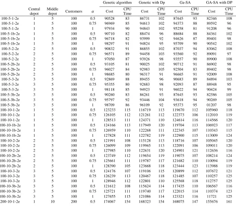
Table 4. Detailed results for Prodhon's instances in large size

Genetic algorithm Genetic with Dp Ga-SA GA-SA with DP

Central depot

Middle

depot Customers 𝛼 Cost

CPU

Time Cost

CPU

Time Cost

CPU

Time Cost

CPU Time

100-5-1-2e 1 5 100 0.5 90528 83 86731 102 87645 93 82346 108

100-5-1-2e 1 5 100 0.75 96969 85 94613 102 94373 88 89592 96

100-5-1-2e 1 5 100 1 97934 90 94843 102 95258 81 91208 96

100-5-1b-2e 1 5 100 0.5 90710 82 88474 96 88684 88 84361 102

100-5-1b-2e 1 5 100 0.75 96718 82 93999 92 94626 87 89401 98

100-5-1b-2e 1 5 100 1 98297 91 94824 95 95709 90 90542 102

100-5-2-2e 2 5 100 0.5 90832 91 86855 102 87037 94 83062 108

100-5-2-2e 2 5 100 0.75 96571 89 94458 103 93560 92 89091 97

100-5-2-2e 2 5 100 1 97050 87 93926 98 93557 90 89900 108

100-5-2b-2e 2 5 100 0.5 93105 81 90025 102 90712 91 86902 98

100-5-2b-2e 2 5 100 0.75 96027 84 92983 105 92504 83 89402 98

100-5-2b-2e 2 5 100 1 98685 80 96317 91 96665 91 92009 108

100-5-3-2e 3 5 100 0.5 92869 88 89455 96 90683 89 84894 103

100-5-3-2e 3 5 100 0.75 95355 80 92683 98 92093 87 88948 95

100-5-3-2e 3 5 100 1 98118 85 94923 91 96022 94 90424 99

100-5-3b-2e 3 5 100 0.5 90260 83 86261 93 87645 93 82586 105

100-5-3b-2e 3 5 100 0.75 95797 92 93446 104 93618 94 90269 105

100-5-3b-2e 3 5 100 1 98709 86 96109 92 95373 95 01207 98

100-10-1-2e 1 5 100 0.5 123233 115 116719 113 119670 112 105960 118

100-10-1-2e 1 5 100 0.75 126105 112 121261 112 122373 106 112010 119

100-10-1-2e 1 5 100 1 128513 111 124371 110 124614 116 114566 120

100-10-1b-2e 1 5 100 0.5 124166 113 117949 120 119704 113 106923 117

100-10-1b-2e 1 5 100 0.75 126959 110 122268 111 122345 107 110343 115

100-10-1b-2e 1 5 100 1 127828 111 122782 119 122900 115 113009 124

100-10-2-2e 2 5 100 0.5 121991 108 115128 113 118716 107 105045 120

100-10-2-2e 2 5 100 0.75 126099 109 119965 113 122091 106 109011 120

100-10-2-2e 2 5 100 1 127985 110 122631 120 124901 121 112636 116

100-10-2b-2e 2 5 100 0.5 123749 112 119654 119 119075 107 108214 124

100-10-2b-2e 2 5 100 0.75 125661 111 119787 117 121682 110 110094 119

100-10-2b-2e 2 5 100 1 128390 105 123668 118 123444 123 113988 119

100-10-3-2e 3 5 100 0.5 124176 107 119106 115 120899 112 107672 121

100-10-3-2e 3 5 100 0.75 126239 113 120467 118 121485 107 110257 125

100-10-3-2e 3 5 100 1 128946 112 122801 110 125568 118 112757 125

100-10-3b-2e 3 5 100 0.5 121612 108 115624 114 117435 110 106567 116

100-10-3b-2e 3 5 100 0.75 125721 111 119740 117 122015 114 110374 123

100-10-3b-2e 3 5 100 1 127655 115 121086 114 123321 116 11721 125

200-10-1-2e 1 10 200 0.5 174067 154 168323 154 168075 147 155676 161

39000 40000 41000 42000 43000 44000 45000 46000

Dataset

1 Dataser2 Dataset3 Dataset4 Dataset5 Dataset6 Dataset7 Dataset8

(21)

Mohammadreza Ghatreh Samani , Seyyed-Mahdi Hosseini-Motlagh

200-10-1-2e 1 10 200 0.75 182085 151 172672 160 176259 140 159064 155

200-10-1-2e 1 10 200 1 187467 144 181091 149 181713 152 170151 163

200-10-1b-2e 1 10 200 0.5 176669 141 167170 146 169890 145 154540 159

200-10-1b-2e 1 10 200 0.75 184859 152 178434 156 178004 148 163401 164

200-10-1b-2e 1 10 200 1 192845 140 184261 156 187094 154 173838 164

200-10-2-2e 2 10 200 0.5 179338 154 172086 159 172000 152 158174 150

200-10-2-2e 2 10 200 0.75 184940 148 176574 158 177402 144 159917 163

200-10-2-2e 2 10 200 1 193829 143 187412 153 189361 149 176823 160

200-10-2b-2e 2 10 200 0.5 178110 146 172082 157 171671 152 157737 157

200-10-2b-2e 2 10 200 0.75 184321 150 175999 151 177437 155 160942 163

200-10-2b-2e 2 10 200 1 194138 151 184657 155 186879 154 173510 153

200-10-3-2e 3 10 200 0.5 174845 140 165346 149 168546 150 152575 160

200-10-3-2e 3 10 200 0.75 181944 154 176330 152 177870 155 163530 155

200-10-3-2e 3 10 200 1 190538 151 181450 149 185284 155 169181 160

200-10-3b 3 10 200 0.5 177568 145 168755 153 172264 142 155968 158

200-10-3b 3 10 200 0.75 182274 140 175238 153 175575 144 159415 159

200-10-3b 3 10 200 1 190989 154 184039 147 186004 148 171927 151

Avg 135007 115 129590 122 130728 117 116919 127

6.1

The Validation of Proposed

Solution Approach

To evaluate the performance of the proposed hybrid solution approach several small-size instances have been investigated in this section and the respective results are reported in Table 5. As can be observed, for instances 1 and 2, the results obtained from solving the concerned problem by the proposed hybrid solution method are the same as the ones obtained by the exact solver GAMS while having remarkably less computing time. However, for instances 3-5, the proposed solution approach achieves the solutions with small gap in comparison to the ones obtained by GAMS. For the problem in larger size the exact solver could not achieve a solution in reasonable length of time while the proposed algorithm performs well as the problem gets larger.

6.2

Sensitivity

Analysis

on

The

Confidence Level

This section aims to investigate the changes in the number of depots by varying service level α. To this aim the problem is solved for instances with 20 customers (small size) and 50 customers (medium size), as shown in Figures 9 and 10. A general observation is that the number of required depots increases as the service level enhances.

Better to say, satisfying higher percentage of customers' total demand generally utilizes the current capacities of existing depots. As long as the capacities of current depots are adequate to respond customer's demands, no more depots will be required. However, the pattern will change if the existing depots cannot be responsible for satisfying customers' demand at the desired level. In such situation, more depots will be added to the current ones so that the desired satisfaction level is met.

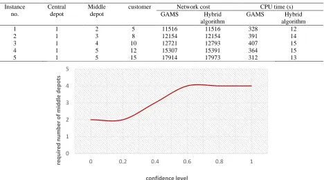
As can be seen in Figure 11, the required number of middle depots will enhance from 2 to 4 as the confidence level increases from zero to 1 in small size. Similarly, the same pattern will be noticed in Figure 12 and the required number of middle depots will reach 5 under confidence level 1 in medium-size problem.

(22)

A Hybrid Algorithm for a Two-Echelon Location-Routing Problem with ….

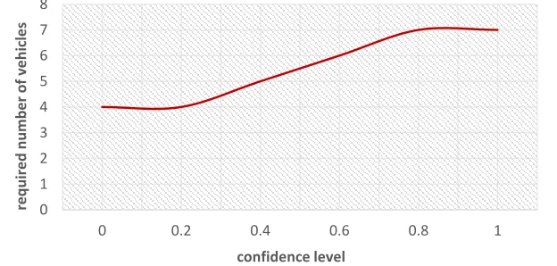
following figures as well. For example, in small-size problem, the number of required vehicles changes from 4 to 7 as the confidence level increases from 0 to 1. With similar pattern, the number of required vehicles increases from 9 to 12 as a result of increasing the confidence level from 0 to 1 in medium size.

6.3

Sensitivity

Analysis

on

The

Capacity of Vehicles

In this section, we analyze the impact of changes in the capacity of vehicles on the cost performance of the network. Figures 13 and 14 depict network cost reduction over different capacity levels for medium-size problem at confidence levelsα= 0.7 and𝛼 = 0.9, respectively. As can be observed in the following diagrams, the increased capacity of vehicles results in decreased network costs. In some parts, however, the curve is steeper which shows reduced network costs and thus increased cost

savings caused by the reduced transportation cost in total since the frequency of transportation decreases when the capacity of vehicles is increased. For instance, at confidence level 0.7, as the increase in capacity level reaches 5%, the amount of cost savings will become about 0.4% while this amount of savings will be 1.2% when the capacity increases to 30%. Consequently, these levels can be noticed as appropriate points for making a considerable reduction in network costs, however, choosing the level of capacity increase based on the decision makers' policies. In some parts, however, the slope of the curve will decrease little by little until it comes to zero and no changes would be seen as the capacity is increased, which means that no capacity shortage has occurred. In other words, the current capacity of vehicles can satisfy the desired amount of demands. Moreover, by increasing the service level from 0.7 to 0.9 the amount of cost savings will decrease resulting from the increase in network costs.

Table 5. summary of results (exact solver versus the proposed hybrid approach)

Instance no.

Central depot

Middle depot

customer Network cost CPU time (s)

GAMS Hybrid

algorithm

GAMS Hybrid

algorithm

1 1 2 5 11516 11516 328 12

2 1 3 8 12154 12154 391 14

3 1 4 10 12721 12793 407 15

4 1 5 12 15307 15391 364 15

5 1 5 15 17914 17973 312 13

Figure. 9. The required number of middle depots under different confidence levels in small size (20-5-1-2e) 0

1 2 3 4 5

0 0.2 0.4 0.6 0.8 1

req

u

ired

n

u

mb

e

r

of mid

d

le

d

e

p

ots

(23)

Mohammadreza Ghatreh Samani , Seyyed-Mahdi Hosseini-Motlagh

81 International Journal of Transportation Engineering, Figure 10. The required number of middle depots under different confidence levels in medium size

(50-5-1-2e)

Figure 11. The required number of vehicles under different confidence levels in small size (20-5-1-2e)

Figure 12. The required number of vehicles under different confidence levels in medium size (50-5-1-2e) 0

1 2 3 4 5 6 7 8

0 0.2 0.4 0.6 0.8 1

req

u

ired

n

u

mb

e

r

of mid

d

le

d

e

p

ots

confidence level

0 1 2 3 4 5 6 7 8

0 0.2 0.4 0.6 0.8 1

req

u

ired

n

u

mb

e

r

of ve

h

icl

e

s

confidence level

0 2 4 6 8 10 12 14

0 0.2 0.4 0.6 0.8 1

req

u

ired

n

u

mb

er

o

f vehicl

es

(24)

Figure 13. The impact of vehicle capacity changes on cost performance; 𝜶 = 𝟎. 𝟕

Figure 14. The impact of vehicle capacity changes on cost performance; 𝜶 = 𝟎. 𝟗

7.

Conclusions and Future

Research Direction

This paper presents a mixed integer programming model for a two-echelon location-routing problem with simultaneous pickup and delivery. To come closer to reality, the amount of demands are considered to be a fuzzy parameter. To handle the demand uncertainty, a fuzzy programming approach based on the credibility theory is devised. A hybrid algorithm based on genetic algorithm (GA) and simulated annealing (SA) algorithm is tailored to solve the proposed model. The results achieved from solving the problem in

different sizes imply that the proposed hybrid algorithm outperforms other algorithms within reasonable length of time. The domination of proposed hybrid algorithm over the other investigated algorithms even strengthens when the size of problem becomes larger. Noteworthy, a comprehensive sensitivity analysis has been performed and several valuable insights have been extracted as follows. (1) our findings from the sensitivity analysis of changes in the capacity of vehicles on the network costs imply that an appropriate increase in the capacity of vehicles can be devised as a strategy to decrease the total cost of network. For example, if the capacity of vehicles is increased up to %10, the system's cost 0

0.5 1 1.5 2 2.5 3

0 5 10 15 20 25 30 35

Cost savin

gs

%

Capacity change %

0 0.3 0.6 0.9 1.2 1.5

0 5 10 15 20 25 30 35

Cost savin

gs

%

(25)

savings will reach nearly %2. (2) fuzzy chance-constrained programming approach provides a confidence level for satisfying the demands such that the number of required vehicles and middle depots to satisfy customer's demands enhances as the confidence level increases. (3) an increase in credibility level would result in increasing total cost, thus, decreasing the cost savings of the network. (4) in comparison to genetic algorithm, the proposed hybrid solution approach generally improves the computing time in small, medium and large sizes of the problem. (5) using a mixed approach of dynamic programming and GA or hybrid approaches will increase the total computing time. A series of future research can be extended in this subject of investigation. For instance, scenario reduction methods could be used to reduce the problem size in large dimensions. Furthermore, using clustering methods could decrease the computing time and the problem complexity. Other heuristic algorithms can be applied to solve the problem and compare the corresponding results with the ones obtained by the proposed algorithm. Researchers could also investigate the problem over a multi period planning horizon considering inventory problem for intermediate depots and customers. A number of approaches such as robust optimization could be devised to handle the data uncertainties.

8. References

-Ambrosino, D. and Scutella, M. (2005) "Distribution network design: new problems and related models", European journal of operational research, Vol. 165, No. 3, pp. 610-624.

-Cheraghi, S., Hosseini-Motlagh, S. M. and Ghatreh Samani, M. R. (2016) "Integrated planning for blood platelet production: a robust optimization approach", Journal of Industrial and System Engineering, Vol. 10 (SI: Healthcare)

-Cheraghi, S. and Hosseini-Motlagh, S. M. (2016) "Optimal blood transportation in disaster relief considering facility disruption and route reliability under uncertainty", International

Journal of Transportation Engineereing Vol. 4, No. 3, pp. 225-254.

-Golozari, F., Jafari, A. and Amiri, M. (2013) "Application of a hybrid simulated annealing-mutation operator to solve fuzzy capacitated location-routing problem", The International Journal of Advanced Manufacturing Technology, Vol. 67, No. 5-8, pp. 1791-1807. -Holland, J. H. (1975) "Adaptation in natural and artificial systems", Ann Arbor, MI: University of Michigan Press.

-Held, M. and Karp, R. M. (1962) "A dynamic programming approach to sequencing problems", Journal of the Society for Industrial and Applied Mathematics, Vol. 10, No. 1, pp. 196-210.

-Hiassat, A., Diabat, A. and Rahwan, I. (2017) "A genetic algorithm approach for location-inventory-routing problem with perishable products", Journal of Manufacturing Systems, Vol. 42, pp. 93-103.

-Hosseini-Motlagh S, Cheraghi, S. and Ghatreh Samani, M. (2016) “A robust optimization model for blood supply chain network design. IJIEPR. Vol. 27, No. 4, pp. 425-444.

-Jacobsen, S. K. and Madsen, O. B. (1980) “A comparative study of heuristics for a two-level routing-location problem", European Journal of Operational Research, Vol. 5, No. 6, pp. 378-387.

-Jokar, A. and Hosseini-Motlagh, S.M. (2015) “Impact of capacity of mobile units on blood supply chain performance: results from a robust analysis”, International Journal of Hospital Research, Vol. 4, No. 3, pp.101-105.

(26)

A Hybrid Algorithm for a Two-Echelon Location-Routing Problem with ….

- Karaoglan, I., Altiparmak, F., Kara, I. and Dengiz, B. (2011) “A branch and cut algorithm for the location-routing problem with simultaneous pickup and delivery”, European Journal of Operational Research, Vol. 211, No. 2, pp. 318-332.

-Laporte G (1988) Location Routing Problems. In: Golden B, Assad A (eds) Vehicle Routing: Methods and Studies, North-Holland, Amsterdam, pp. 293–318

-Liu, B. and Liu, Y. K. (2002) "Expected value of fuzzy variable and fuzzy expected value models", IEEE Transactions on fuzzy systems, Vol. 10, No. 4, pp. 445-450.

-Madsen, O. (1983) "Methods for solving combined two level location-routing problems of realistic dimensions", European Journal of Operational Research, Vol.12, No. 3, pp. 295-301.

-Majidi, S., Hosseini-Motlagh, S. M., Yaghoubi, S. and Jokar, A. (2017) " Fuzzy green vehicle routing problem with simultaneous pickup delivery and time windows", RAIRO-Operations Research.

DOI:https://doi.org/10.1051/ro/2017007. -Majidi, S., Hosseini-Motlagh,S. M. and Ignatius, J. (2017) "Adaptive large neighborhood search heuristic for pollution routing problem with simultaneous pickup and delivery", Soft Computing.

DOI:https://doi.org/10.1007/s00500-017-2535-5

-Min, H., Jayaraman, V. and Srivastava, R. (1998) "Combined location-routing problems: A synthesis and future research directions", European Journal of Operational Research, Vol.108, No. 1, pp. 1-15.

-Nadizadeh, A. and Hosseini Nasab, H. (2014) "Solving the dynamic capacitated location-routing problem with fuzzy demands by hybrid heuristic algorithm", European Journal of Operational Research, Vol. 238, No. 2, pp. 458-470.

-Nagy, G. and Salhi, S. (2007) "Location-routing: Issues, models and methods", European Journal of Operational Research, Vol. 177, No. 2, pp. 649-672.

-Nambiar, J. M., Gelders, L. F. and Van Wassenhove, L. N. (1981) "A large scale location-allocation problem in the natural rubber industry", European Journal of Operational Research, Vol. 6, No. 2, pp. 183-189.

-Nikbakhsh, E. and Zegordi, S. H. (2010) "A heuristic algorithm and a lower bound for the two-echelon location-routing problem with soft time window constraints", Scientia Iranica Transaction E: Industrial Engineering, Vol. 17, No. 1, pp. 36-47.

-Nikkhah Qamsari, A. S., Hosseini-Motlagh, S. M., and Jokar, A. (2017) "A two-phase hybrid heuristic method for a multi-depot inventory-routing problem", International Journal of Transportation Engineering, Vol. 4, No. 4, pp. 284-304.

-Prodhon, C. and Prins, C. (2014) "A survey of recent research on location-routing problems", European Journal of Operational Research,Vol. 238No. 1, pp. 1-17.

-Riahi, N., Hosseini-Motlagh, S. M. and Teimourpour, B. (2013) " Three-phase Hybrid times series modeling framework for improved hospital inventory demand forecast" International Journal of Hospital Research Vol. 2, No. 3, pp. 130-138.

(27)

Mohammadreza Ghatreh Samani , Seyyed-Mahdi Hosseini-Motlagh

-Riquelme-Rodríguez, J., Gamache, M. and Langevin, A. (2016) " Location arc routing problem with inventory constraints", Computers and Operation Research, Vol. 76, pp. 84-94. -Schiffer, M. and Walther, G. (2017) "The electric location routing problem with time windows and partial recharging", European Journal of Operational Research.

DOI:https://doi.org/10.1016/j.ejor.2017.01.011. -Tavakkoli-Moghaddam, R., Raziei, Z. and Tabrizian, S. (2016) "Solving a bi-objective multi-product vehicle routing problem with heterogeneous fleets under an uncertainty condition", International Journal of Transportation Engineering, Vol. 3, No. 3, pp. 207-225.

-Wasner, M. and Zapfel, G. (2004) "An integrated multi-depot hub-location vehicle routing model for network planning of parcel

service", International Journal of Production Economics, Vol. 90, No. 3, pp. 403-419.

-Watson-Gandy, C. D. T. and Dohrn, P. J. (1973) "Depot location with van salesmen a practical approach", Omega, Vol. 1, No. 3, pp. 321-329. -Webb, M. H. J. (1968) "Cost functions in the location of depots for multiple-delivery journeys", Journal of the Operational Research Society, Vol.19, No. 3, pp.311-320.

-Zarandi, M. H. F., Hemmati, A., Davari, S., and Turksen, I. B. (2013). “Capacitated location-routing problem with time windows under uncertainty”, Knowledge-Based Systems, Vol.37, pp. 480-489.

DOI:https://doi.org/10.1016/j.ejor.2017.01.011.