Int. J. Data Envelopment Analysis (ISSN 2345-458X)
Vol.7, No.3, Year 2019 Article ID IJDEA-00422, 14 pages Research Article
Determination of Right/Left return to Scale in
Two-Stage Processes Based on Dual Simplex
S. Fanati Rashidi*
Department of Mathematics, Shiraz Branch, Islamic Azad University, Shiraz, Iran
Received 23 March 2019, Accepted 20 July 2019
Abstract
As a non-parametric method of relative efficient measurement of a group of decision making units ( ), Data Envelopment Analysis (DEA) is one of the most important tools in efficiency computation. One of the main concerns dealt with in DEA is dealing with return to scale in two-stage processes in which, produced outputs of the first stage inputs are used as inputs for the second stage. The outputs of the first stage are considered as the intermediate products. Therefore, the second stage uses these intermediate products for producing the outputs of the same stage. Based on this construction, the total process can be analyzed for efficiency production from two sub-processes. In this paper, a new model is proposed that eliminates the defections of the previous models and is used to determine the right and left return to scale in two-stage processes of decision making units.
Keywords: Efficiency, Two-stage processes, Return to scale.
*. Corresponding author: Email: [email protected]
1. Introduction
Nowadays, units’ calculation and comparison are one of the most important fields in economy that act cooperatively in the same field. Charnes et al. [1] have proposed a practical model to calculate and compare the efficiency of decision making that could calculate the efficiency of the units with various inputs and outputs. During 1970s, the field has attracted many attention and been developed to a great extent and different models have been proposed by experts in different areas. One of those areas is multi-stage decision making units. For example, Charnes et al. [2] faced a problem similar to a two-stage decision making, in which two-stage method must be used for army employment. Later on, Schinnar et al. [3], Sexton and Lewise [4], Chen and Zhu [5], and Liang et al. [6] applied two-stage DEA in mental health care, baseball, information technology, and evaluation the performance of supply chain, respectively. So far, various scientists have studied this field. For instance, Izadikhah and Saen [7], Kalhor and Kazemi matin [8]. Kao and Hwang [9] have proposed a different model by which the efficiency of the whole systems is decomposed into the efficiency of two systems. This model has been proposed based on the assumption of return to scale. Chen et al. [10] have proposed a model similar to Kao and Hwang [9], in which constant return to scale and variable return to scale were studied. Later, Chen et al. [11] and Kao and Hwang in [12] developed their proposed models.
Despotis et al. [13] proposed a new definition of system efficiency in two-stage process. It was based on weak link in supply chain, maximum flow algorithm, and minimal cut theorem for networks. Hatami-Marbini et al. [14] and Alirezaee et al. [15] introduced new approaches in return to scale in data envelopment analysis.
In this paper, it is purposed to introduce a new model for two-stage DEA. Considering both the importance of return to scale and the defects of the other mentioned proposed models in two-stage DEA, return to scale of two-stage model is discussed by the use of right and left return to scale that was studied by Golany and Yu [16] and Hadjicostas and Soteriou [17]. This study is done using the proposals of Zarepisheh and Soleimani-damaneh [18]. Other parts of this paper are as follows. Section 2 is devoted to literature review of two-stage processes. The organization of the paper is in the following way. Our recommended model is presented in section 3. In the section 4, return to scale in two-stage DEA is calculated with the proposed model. Finally, a numerical example is solved in section 5 and the section 6 is devoted to conclusions.
2. Review
Consider n decision making units that each ( ∈ = {1, … , }) generates the q outputs of ( = 1, … , ) using m inputs of ( = 1, … , ) and then the obtained q outputs would be the inputs for generating s outputs of ( = 1, … , ). Hwang and Kao [19] have used two-stage DEA of Seiford and Zhu [20] to measure the total efficiency as well as the efficiency of the first and the second stage. Also, they have introduced the efficiency of the first and the second stage by assuming constant return to scale as follows:
= max ∑ w ∑ v x . . ∑ w z ∑ v x ≤ 1, j = 1, … , n, (1)
, ≥ , = 1, … , ; = 1, … , ,
And the efficiency score of the second stage has been introduced as follows:
3
j = 1, … , n, (2)
, ≥ , = 1, … , ; = 1, … , . In which, was a small non-Archimedean number and , and were weight of inputs, intermediate products and outputs, respectively. The efficiency of each stage in models (1) and (2) were calculated independently. Kao and Hwang [9] have proposed their new model as a relational model by using intermediate products and assuming constant return to scale and the equality of weights in intermediate products of data envelopment. The overall efficiency score of the relational model was calculated as follows: = max ∑ ⁄∑ . . ∑ ⁄∑ ≤ 1,
= 1, … , , ∑ w z ∑ v x ≤ 1, j = 1, … , n, (3)
∑ u y ∑ w z ≤ 1, j = 1, … , n, , و ≥ , = 1, … , ;
= 1, … , ; = 1, … , .
The set of limitations in model (3) were in fact the set of limitations of models (1) and (2). So, the overall efficiency was = × . Indeed, in their relational model, the overall efficiency score was the multiplication of the first and the second stages. But, as multiplication of two numbers between 0 and 1 leads to a smaller one, the result was not a true representation of efficiency score. Moreover, in Hwang and Kao independent model [19], two models are independently solved and this is not logical for the decision making units with a common decision maker. As the proposed model by Kao and Hwang [9] was in the form of constant return to scale, Chen et al. [10] introduced their model in form of constant return to scale and variable return to scale. Considering the complex computation of this model and the large number of variables and constants, calculating the return to scale of decision making units is a difficult task. In the next section, a new model is proposed that is less complex. 3. Proposed model According to what mentioned above, a new model is proposed here to calculate the efficiency of decision making units with different stages. Similar to the dependent model introduced by Kao Hwang [9], in this model, intermediate production is considered equal without taking the roles of the inputs and outputs into account and is entered into the model as one intermediate production. In this paper it is tried to calculate the efficiency of each stage simultaneously by considering the roles of the input and the output. The envelopment form of the model based on the output oriented is as follows: max . . ∑ ≤ , = 1, … , ,
∑ ≥ , = 1, … , ,
∑ = 1,
∑ ≤ , = 1, … , , (4)
∑ ≥ , = 1, … , ,
∑ = 1,
≥ 0, ≥ 0, = 1, … , .
Considering the corresponding variables of , , with constraints of model (4), the dual model is presented as follows: ∑ + ∑ + + . . ∑ − ∑ + ≥ 0,
= 1, … , , ∑ − ∑ − ≥ 0, = 1, … , , (5)
∑ + ∑ = 1,
= 1, … , , = 1, … , , = 1, … , .
4. Return to scale in two- stage DEA In this section, it is tried to develop the proposed model using the presented suggestions by Zarepisheh and Soleimani-damaneh [18].
In this model,
= , , … , , Z
= z , , … , , = ( , , … , )
are defined as the vectors of input, intermediate and output of , respectively. Also,
= [ , , … , ],
= [ , , … , ], = [ , , … , ]
are × , × , and × matrices of inputs, intermediate productions and outputs, respectively. According to the proposed model, production possibility is defined as follows:
=
⎩ ⎪ ⎪ ⎪ ⎪ ⎪ ⎪ ⎪ ⎪ ⎪ ⎨ ⎪ ⎪ ⎪ ⎪ ⎪ ⎪ ⎪ ⎪ ⎪ ⎧
( , , ) ∈
∃( , ) ∈ :
≤ ,
≥ ,
= 1,
≥ 0,
≤ ,
≥ ,
= 1,
≥ 0. ⎭
⎪ ⎪ ⎪ ⎪ ⎪ ⎪ ⎪ ⎪ ⎪ ⎬ ⎪ ⎪ ⎪ ⎪ ⎪ ⎪ ⎪ ⎪ ⎪ ⎫
Where, o and e are two vectors with zero and one component, respectively. Based on the proposed model, the efficiency of the decision making unit, like in output oriented, is evaluated as follows:
Definition 1. is defined as the technical efficient unit in output oriented if ∗= 1 (where ‘*’ shows optimality). For the inefficient units, according to Banker et al. [21], they can be used in RTS evaluation by being projected in the efficient frontier. Here, the projection points are defined as follows:
= , = ∗ , = ∗
As a result, in order to determine constant return to scale, ( , , ) must be replaced by ( , , ); therefore, to determine RTS of the proposed model, the following limits can be used (see Hadjicostas, Soteriou [17]).
ρ = limβ→ α(β)
β ,
ρ = limβ→ α (β)
β (6)
The function α(β) corresponding to is
α(β) = max{α|(β , , ) } (7)
Notification 1. According to model (4) and α definition, α(β) can be supposed as the optimal value of model (4) in which β is placed in input as a substitution of . By accepting this issue and model (7), it is clear that if β= 1 , the researcher wants to solve model (4) for vectors of the inputs and outputs ( , , ). Therefore, considering the projection points ( , , ) and the fact that α is optimal for model (4) along with ( ,α ,α ) vector has been projected on the efficient frontier, it can be concluded that α(1) = 1.
Assumption 1. As mentioned in Hadjicostas and Soteriou [17], η∈ [0,1),γ≥ 0 exists such that
η , , ∈ .
5
Lemma 1. If α(1) = 1, exists and is finite.
Proof: To prove the following assumption, there is:
Assumption 1: convexity
( , ) ∈ , ′, ′ ∈ , ⟹ ( +
(1 − ) ′, + (1 − ) ′) ∈
Assumption 2: Monotonicity ( , ) ∈ , ′≥ , 0 ≤ ′≤
′, ′ ∈ × ⟹ ′, ′ ∈
Assumption 3: Inclusion of observations ∈ exists and , are exist too such that for each j = 1, … , n the observation of ( , ) ∈ are related to
.
Assumption 4: Minimum extrapolation If a set preserves the possibility of
production of assumptions 1, 2, and 3 (for n observations(( , )، = 1, … , ), then ⊆ . Now, if 3 and 4 are appointed, exists and is finite.
Lemma 2: If α(1) =1and assumption 1 is determined, ρo exists and is finite.
Proof: If α(1) =1and assumption 1 is determined, the following limits exist and are finite.
ρo = lim
β→1
α(β) −1
β−1 ,ρo =βlim→1
α(β) −1 β−1
Here, assumption 1 is determined. The proposed model is convex because it is the products of two conceive sets.
Definition 2: in is increasing from right (constant, decreasing) if ρ > 1(= 1, < 1) and is decreasing if ρ > 1(= 1, < 1).
If assumption 1 is not determined, it means that reduction with the same proportion of inputs in is impossible. In this situation,
contraction cannot be discussed and, consequently, RTS cannot be defined for left.
Now, in order to calculate and ρ according to Hadjicostas and Soteriou [17], we can act as follows.
First model (4) must be solved. Then, ρ and ρ can be calculated after the linear program model has been solved.
ρ = 1 − α∗
α∗= max u + u
. . ∑ − ∑ + ≥ 0,
= 1, … , ,
∑ − ∑ − ≥ 0,
= 1, … , , (8)
∑ ̂ + ∑ = 1,
u + u + ∑ + ∑ ̂ = 1,
u ≥ 0, u ≥ 0.
And ρ = 1 − ∗is defined as follows: ∗= u + u
. . ∑ − ∑ + ≥ 0,
= 1, … , ,
∑ − ∑ − ≥ 0,
= 1, … , , (9)
∑ ̂ + ∑ = 1,
u + u + ∑ + ∑ ̂ = 1,
u ≥ 0, u ≥ 0.
x , ̂ , were introduced before.
Theorem 1: If α(1) =1and matrix B is an optimal base for model (4) as:
⎝ ⎜ ⎜ ⎜ ⎛ B
⎝ ⎜ ⎜ ⎛
x
O×
O ×
1
1 ⎠
⎟ ⎟ ⎞
, B
⎝ ⎜ ⎜ ⎛
x
O×
O ×
0
0 ⎠
⎟ ⎟ ⎞
⎠ ⎟ ⎟ ⎟ ⎞
So,ρ = B ⎝ ⎜ ⎜ ⎛ x O× O × 0 0 ⎠ ⎟ ⎟ ⎞
in that
shows the target function coefficient vector corresponding to basis B in model (4). Proof: Put = B ⎝ ⎜ ⎜ ⎛ x Z O× O × 1 1 ⎠ ⎟ ⎟ ⎞ , = B ⎝ ⎜ ⎜ ⎛ x Z O× O × 0 0 ⎠ ⎟ ⎟ ⎞
Define = ∞ if ≥ 0; otherwise,
= min ∶ ∈ {1, … , + + 1}, < 0
Because , ≥ 0, we have ̅ > 0, + δ ≥ 0 .
For each δ∈ 0, ̅ and
B
⎝ ⎜ ⎜ ⎛
(1 + δ)x (1 + δ)Z O× O × 1 1 ⎠ ⎟ ⎟ ⎞
≥ 0,
for each δ∈ (0, ̅), it means that B is an optimal basis for model (4) that corresponds to ((1 + δ)x , (1 + δ)Z , Y ). Optimality of basis is separated from RHS vector and, as a result, B is the optimal basis for model (4) that is corresponding to ((1 + δ)x , (1 + δ)Z , Y ). Put = 1 + , ̅ = 1 + δ. According to notification 1, for ∈ (1, ̅), it is concluded that
α(β) = B
⎝ ⎜ ⎜ ⎜ ⎛ x Z O× O × 1 1 ⎠ ⎟ ⎟ ⎟ ⎞ .
The equality of α(1) = 1 leads to
B ⎝ ⎜ ⎜ ⎛ x Z O× O × 1 1 ⎠ ⎟ ⎟ ⎞
= 1, so:
α(β) = B
⎝ ⎜ ⎜ ⎜ ⎛
1 + − 1 x 1 + − 1 Z
O× O × 1 1 ⎠ ⎟ ⎟ ⎟ ⎞ = B ⎝ ⎜ ⎜ ⎛ x Z O× O × 1 1 ⎠ ⎟ ⎟ ⎞ +
(β − 1) B
⎝ ⎜ ⎜ ⎛ x Z O× O × 0 0 ⎠ ⎟ ⎟ ⎞ ⇒
α(β) = 1 + (β − 1) B
⎝ ⎜ ⎜ ⎛ x Z O× O × 0 0 ⎠ ⎟ ⎟ ⎞
⇒ ( ) = B
⎝ ⎜ ⎜ ⎛ x Z O× O × 0 0 ⎠ ⎟ ⎟ ⎞ .For each
β ∈ (1, β) ⇒
ρ = B
7
Theorem 2: if α(1) = 1 and matrix B is an optimal basis for model (4) as
⎝ ⎜ ⎜ ⎜ ⎜ ⎜ ⎜ ⎜ ⎜ ⎛ B
⎝ ⎜ ⎜ ⎛
x
O×
O ×
1
1 ⎠
⎟ ⎟ ⎞ ,
B
⎝ ⎜ ⎜ ⎛
−x − O×
O ×
0
0 ⎠
⎟ ⎟ ⎞
⎠ ⎟ ⎟ ⎟ ⎟ ⎟ ⎟ ⎟ ⎟ ⎞
≽ 0, (11)
so, ρ = B
⎝ ⎜ ⎜ ⎛
−x − O× O ×
1
1 ⎠
⎟ ⎟ ⎞
.
Proof: The proof of this theorem is similar to the previous one. In this case, it
should be = B
⎝ ⎜ ⎜ ⎛
−x −z O× O ×
0
0 ⎠
⎟ ⎟ ⎞
.
Figure 1 shows the different stages of the proposed method for obtaining left and right return to scale (RTS).
Figure 1: The algorithm to obtain left and right RTS based on the proposed model
RTS in DMUo is
constant if = 1
RTS in DMUo is
decreasing from left if > 1
RTS in DMUo is
decreasing from right if
< 1
RTS in DMUo is
constant if = 1
RTS in DMUo is
increasing from right if
> 1
Solving proposed model (4)
Obtaining α(β) from Eq. 6
Obtaining from Eq. 10 and
from Eq. 11
will be existent and finite if α(1)=1 and assumption 1 is
valid.
RTS in DMUo is
increasing from left if
< 1
will be existent and finite if α(1)=1 and assumptions 3
5. Numerical Example 5.1 Example 1
Table 1 shows the data of 24 branches of none-life insurance company of Taiwan from Hwang and Kao [19]. The inputs of the first process are operation and insurance costs. On the other hand, the outputs of the first process that are intermediate production are direct written premiums and reinsurance premiums that are the inputs of the second stage. Finally, the outputs of the second stage are underwriting profit and investment profit. Table 2, shows the amount of the
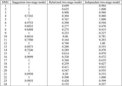
efficiency of Hwang and Kao [19], independent model Kao and Hwang [9] dependent model, and the proposed model. In Kao and Hwang [9] dependent model, none of units are efficient. In the independent model, on the other hand, some of the units are efficient, while none of sub-processes are efficient. As it can be seen in the proposed model, most of the units are efficient and the inefficient units have similar efficiency, that leads to a better outcome compared to independent and dependent models.
Table1: Input (x), intermediate production (z), and output (y) of 24 branches of none-life insurance company of Taiwan
Investment profit (y2) Underwriting profit (y1) Reinsurance premiums (z2) Direct written premiums (z1) Insurance expenses (x2) Operation expenses (x1) DMU 681687 834754 658428 177331 3925272 415058 439039 622868 264098 554806 18259 909295 223047 332283 555482 197947 371984 163927 46857 26537 6491 4181 18980 16976 477733 984143 1228502 293613 248709 7851229 1713598 2239593 3899530 1043778 1697941 1486014 1574191 3609236 140100 3355197 854054 3144484 692731 519121 355624 51950 82141 0.1 142370 1602873 856735 1812894 560244 371863 1753794 952326 643412 1134600 546337 504528 643178 1118489 811343 465509 749893 402881 342489 995620 483291 131920 40542 14574 49864 644816 667964 7451757 10020274 4776548 3174851 37392862 9747908 10685457 17267266 11473162 8210389 7222378 9434406 13921464 7396396 10422297 5606013 7695461 3631484 1141950 316829 225888 52063 245910 476419 7832893 673512 1352755 592790 594259 3531614 668363 1443100 1873530 950432 1298470 672414 650952 1368802 988888 651063 415071 1085019 547997 182338 53518 26224 10502 28408 235094 828963 1178744 1381822 1177494 601320 6699063 2627707 1942833 3789001 1567746 1303249 1962448 2592790 2609941 1396002 2184944 1211716 1453797 757515 159422 145442 84171 15993 54693 163297 1544215 1. Taiwan Fire
2. Chung Kuo 3. Tai Ping 4. China Mariners
5. Fubon 6. Zurich 7. Taian 8. Ming Tai
9. Central 10. The First 11. Kuo Hua 12. Union 13. Shingkong 14. South China 15. Cathay Century 16. Allianz President
17. Newa 18. AIU 19. North America
20. Federal 21. Royal&Sun alliance
22. Asia 23. AXA 24. Mitsui Sumitomo
9
Table 2: The amount of the efficiency of independent, dependent, and proposed models for 24 branches of none-life Company.
Independent two-stage model Relational two-stage model
Suggestion two-stage model DMU
0.984 1.000 0.988 0.488 1.000 0.594 0.470 0.415 0.327 0.781 0.283 1.00 0.353 0.470 0.979 0.472 0.635 0.427 0.822 0.935 0.333 1.000 0.599 0.257 0.699
0.625 0.960 0.304 0.767 0.390 0.277 0.275 0.223 0.46 0.164 0.760 0.208 0.289 0.614 0.320 0.360 0.259 0.411 0.547 0.20 0.590 0.420 0.135 1
1 1 0.7243
1 0.9753 0.8032 0.8404
1 0.8616 0.7580
1 0.8873 0.7246
1 0.9099
1 1 1 1 0.8950
1 0.9855
1 1
2 3 4 5 6 7 8 9 10 11 12 13 14 15 16 17 18 19 20 21 22 23 24
5-2 Example 2
To investigate the proposed method for left/right return to scale, we use the following illustrative example:
Suppose that we have one input, one intermediate measure, and one output (m=s=q=1). Data is given in Table 3. First, we consider the as the under evaluation unit. The corresponding model (4) to this DMU is as follows and optimal
solution of this problem is shown in table of (4):
=
. . 2 + 3 + 4 + 5 ≤ 2, 2 + 4 + 3 + 5 ≥ 2α,
+ + + = 1,
2μ + 4μ + 3μ + 5μ ≤ 2, 2μ + 5μ + 3μ + 5μ ≥ 2α, μ + μ + μ + μ = 1,
≥ 0, ≥ 0, j = 1, … ,4, α is free.
Table 3: Input, output, and intermediate data Y Z
X DMU
2 2
2 A
5 4
3 B
3 3
4 C
5 5
Table 4: Optimal Simplex table from solving model (4) for
Α μ μ μ μ μ μ RHS SRHS
Z 0 0 0 0 0 0 0 0 0 1/4 ¾ 3/4 1/2 1 3/2
0 0 1 1 0 2/3 1/3 0 0 -1/6 -1/2 -1/2 -1/3 0 1/3 α 0 0 0 0 1 0 0 0 0 1/4 ¾ 3/4 1/2 1 3/2 1 0 1 0 0 1/3 2/3 0 0 -1/3 -1 -1 -2/3 1 -4/3
μ 0 0 0 0 0 0 0 0 1 1/2 3/2 1/2 0 0 1
0 1 -1 0 0 -1 -1 0 0 1/2 3/2 3/2 1 0 1
μ 0 0 0 0 0 0 0 1 0 1/2 -1/2 -1/2 0 1 -1
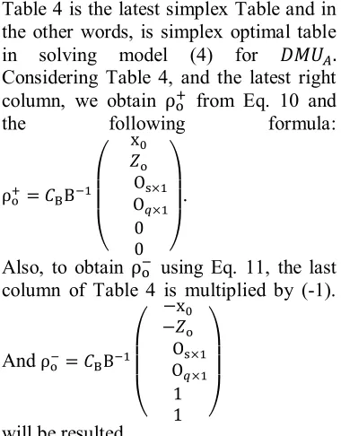
Table 4 is the latest simplex Table and in the other words, is simplex optimal table in solving model (4) for . Considering Table 4, and the latest right column, we obtain ρ from Eq. 10 and
the following formula:
ρ = B
⎝ ⎜ ⎜ ⎛
x
O× O ×
0
0 ⎠
⎟ ⎟ ⎞
.
Also, to obtain ρ using Eq. 11, the last column of Table 4 is multiplied by (-1).
And ρ = B
⎝ ⎜ ⎜ ⎛
−x − O× O ×
1
1 ⎠
⎟ ⎟ ⎞
will be resulted.
Notice that , , μ and μ are the co-variants of 1, 2, 3, 4 and 5 limitations in Table (4). and μ are the artificial variables of equal constrains. In table (4) it can be seen that, if we consider RHS and SRHS columns, we have condition (10) and we have = 3/2. Also, in order to calculate , we consider table (4), multiplying SRHS in(-1), the result would be table (5). In this table, it can be seen that the corresponding lines to , μ and are orderly (0,-1/3), (0,-1) and (0,-1) and we don’t have the condition (11) therefore, it is not possible to apply the dual simplex.
Now we consider the . Table (6) shows the obtained optimal table of the model (4), which corresponds to this DMU.
Table 5: Multiplication the SRHS in Table 4 by -1 to obtain
Α μ μ μ μ μ μ RHS SRHS
Z 0 0 0 0 0 0 0 0 0 1/4 3/4 3/4 1/2 1 3/2
0 0 1 1 0 2/3 1/3 0 0 -1/6 -1/2 -1/2 -1/3 0 -1/3
Α 0 0 0 0 1 0 0 0 0 1/4 3/4 3/4 1/2 1 -3/2
1 0 1 0 0 1/3 2/3 0 0 -1/3 -1 -1 -2/3 1 4/3
μ 0 0 0 0 0 0 0 0 1 1/2 3/2 1/2 0 0 -1
0 1 -1 0 0 -1 -1 0 0 1/2 3/2 3/2 1 0 -1
11
Table 6: Optimal Simplex table from solving model (4) for
α μ μ μ μ μ μ RHS SRHS
Z 0 0 0 0 0 0 1/3 0 0 1/6 1/2 1/2 1/3 7/6 2
0 0 3/2 3/2 0 1 0 0 0 -1/4 -3/4 3/4 -1/2 11/4 7
Α 0 0 0 0 1 0 1/3 0 0 1/6 1/2 1/2 1/3 7/6 2
1 0 1/2 -1/2 0 0 0 0 0 -1/4 -3/4 3/4 -1/2 7/4 3
μ 0 0 0 0 0 0 0 0 1 1/2 3/2 1/2 0 1/2 2
0 1 1/2 3/2 0 0 0 0 0 1/4 3/4 3/4 1/2 3/4 3
μ 0 0 0 0 0 0 0 1 0 1/2 -1/2 -1/2 0 1/2 -2
Table 7: Multiplication the SRHS in Table 6 by -1 to obtain
α μ μ μ μ μ μ RHS SRHS
Z 0 0 0 0 0 0 1/3 0 0 1/6 1/2 1/2 1/3 7/6 2
0 0 3/2 3/2 0 1 0 0 0 -1/4 -3/4 3/4 -1/2 11/4 -7
Α 0 0 0 0 1 0 1/3 0 0 1/6 1/2 1/2 1/3 7/6 -2
1 0 1/2 -1/2 0 0 0 0 0 -1/4 -3/4 3/4 -1/2 7/4 -3
μ 0 0 0 0 0 0 0 0 1 1/2 3/2 1/2 0 1/2 -2
0 1 1/2 3/2 0 0 0 0 0 1/4 3/4 3/4 1/2 3/4 -3
μ 0 0 0 0 0 0 0 1 0 1/2 -1/2 -1/2 0 1/2 +2
It is obvious that, considering RHS and SRHS columns, we have the condition (10) and also = 2. To obtain the , we consider the table (6). Multiplying to (-1) we try to have the condition (11). The result is the table (7) with result = 2.
6- Conclusion
In this paper, different methods have been shown for measuring efficiency and return to scale in two-stage processes. So far, many methods for efficiency evaluation and network return to scale have been proposed, each contains pros and cons. One of the problems in determining network return to scale is the feasibility of the proposed method. For example, the proposed method by Golany and Yu, [16] is not always feasible, but our approach is always feasible for all DMUs under evaluation.
In addition, in many other network approaches, two independent models are considered to evaluate the efficiency of
network processes. Such as, independent model of Kao and Hwang [9] which two independent models will result in two independent efficiency frontiers. Indeed, we can hardly find a common approach for return to scale of units between these two frontiers. Although Kao and Hwang [9] evaluated the whole process efficiency, their model was only considered in constant return to scale condition.
13
References
[1] Charnes, A., Cooper, W.W., & Rhodes, E. (1978). Measuring the efficiency of decision making units. European Journal of Operational Research, 2, 429-444.
[2] Charnes, A., Cooper, W.W., Golany, B., Halek, R., Klopp, G., Schmitz, E., & Thomas, D. (1986). Two Phase Data Envelopment Analysis Approach to Policy Evaluation and Management of Army Recruiting Activities: Tradeoffs between Joint Services and Army Advertising. Research Report CCS no, 532, Center for Cybernetic studies, The University of Texas at Austin Texas.
[3] Schinnar, A.P., Kamis-Gould, E., Delucia, N., & Rothbard, A.B. (1990). Organizational determinants of efficiency and effectiveness in mental health partial care Programs. Health Services Research, 25, 387-420.
[4] Sexton, T.R., & Lewis, H.F. (2003). Two-stage DEA: An application to major league baseball. Journal of Productivity Analysis, 19, 227-249.
[5] Chen, Y., & Zhu, J. (2004). Measuring information technologies indirect impact on firm performance. Information Technology & Management Journal, 5, 9-22.
[6] Liang, L., Yang, F., Cook, W.D., & Zhu, J. (2006). DEA model for supply chain efficiency evaluation. Annals of Operations Research, 145, 35-49.
[7] Izadikhah M, Saen RF.(2016), Evaluating sustainability of supply chains by two-stage range directional measure in the presence of negative data. Transportation Research Part D:
Transport and Environment. 2016; 11: 111-26.
[8] Kalhor. A, Kazemi Matin. R, (2017), Performance evaluation of general network production processes with undesirable outputs: A DEA approach, RAIROO per. Res. DOI: https:// doi.org/ 11.1151/ ro/2017122.
[9] Kao, C., & Hwang, S.N. (2008). Efficiency decomposition in two-stage data envelopment analysis: An application to non-life insurance companies in Taiwan. European Journal of Operational Research, 185, 418-429.
[10] Chen, Y., Cook, W.D., Li, N., & Zhu, J. (2009). Additive efficiency decomposition in two-stage DEA. European Journal of Operational Research, 196, 1170-1176.
[11] Chen, Y., Cook, W.D., & Zhu, J. (2010). Deriving the DEA frontier for two-stage processes. European Journal of Operational Research, 202, 138-142.
[12] Kao, C., & Hwang, S.N. (2011). Decomposition of technical and scale efficiencies in two-stage production systems. European Journal of Operational Research, 211, 515-519.
[13] Despotis, D. K., Koronakos, G., & Sotiros, D. (2016b). The “weak-link” approach to network DEA for two-stage processes. European Journal of Operational Research, 254, 481-492.
[15] Alirezaee , A., Hajinezhad, E. , Paradi, J. C. ,(2018), Objective identification of technological returns to scale for data envelopment analysis models , European Journal of Operational Research , Pages 678-688.
[16] Golany, B., & Yu, G. (1997). Estimating returns to scale in DEA. European Journal of Operational Research, 103, 28-37.
[17] Hadjicostas, P., & Soteriou, A.C. (2006). One-sided elasticities and technical efficiency in multi-output production: A theoretical framework. European Journal of Operational Research, 168, 425-449.
[18] Zarepisheh, M., & Soleimani-damaneh, M. (2009). A dual simplex-based method for determination of the right and left returns to scale in DEA. European Journal of Operational Research, 194, 585-591.
[19] Hwang, S.N., & Kao, T.L. (2006). Measuring managerial efficiency in non-life insurance companies: An application of two-stage data envelopment analysis technique. International Journal of Management, 23, 699-720.
[20] Seiford, L.M., & Zhu, J. (1999). Profitability and marketability of the top 55 US commercial banks. Management Science, 45, 1270-1288.
[21] Banker, R.D., Bardhan, I., & Cooper, W.W. (1996). A note on returns to scale in DEA. European Journal of Operational Research, 88, 583-585.
[22] Davtalab. M., Olyaie, I., Roshdi. V., Partovi Nia. M., Asgharian, (2014). On characterizing full dimensional weak facets in DEA with variable returns to scale technology. Optimization: A Journal