University of Mazandaran, Iran http://cjms.journals.umz.ac.ir ISSN: 1735-0611 CJMS.3(2)(2014), 253-265
The Bernoulli Ritz-collocation method to the solution of modelling the pollution of a system of lakes
E. Sokhanvar 1 and S. A. Yousefi2
1 Department of Mathematics, Kerman Graduate University of
Technology, Kerman, Iran
2 Department of Mathematics, Shahid Beheshti University , Tehran,
Iran
Abstract. Pollution has become a very serious threat to our envi-ronment. Monitoring pollution is the first step toward planning to save the environment. The use of differential equations, monitor-ing pollution has become possible. In this paper, a Ritz-collocation method is introduced to solve modelling the pollution of a system of lakes by a system of differential equations. The method is based upon Bernoulli polynomials. These polynomials are first presented. The Bernoulli Ritz-collocation method is then utilized to reduce modelling the pollution of a system of lakes to the solution of alge-braic equations. An illustrative example is included to demonstrate the validity and applicability of the proposed method.
Keywords: Bernoulli polynomials; modelling the pollution of a system of lakes; Ritz-collocation method.
2000 Mathematics subject classification: xxxx, xxxx; Secondary xxxx.
1. Introduction
Most physics and biology events can be modeled by the differential, integral and integro-differential equations. Since few of these equations cannot be solved analytically, so numerical method is requested [1, 2, 3,
1Corresponding author: [email protected] Received: 25 November 2013
Revised: 3 February 2014 Accepted: 2 March 2014
4, 5, 6, 7, 8]. Polynomial series and orthogonal functions are incredibly useful mathematical tools for solving these problems. In recent years, the Taylor, Chebyshev, Legendre, Bernoulli and Bessel ( Ritz-collocation and matrix) methods have been used to find the approximate solutions of differential, integral and integro-differential-difference equations and their systems [9, 10, 11, 12, 13, 14, 15].
In this paper, we introduce the Bernoulli Ritz-collocation method for solving modelling the pollution of a system of lakes. In 2006, Biazar et. al analyzed this model [16]. Recently, this model was solved using the variational iteration method [17], the homotopy perturbation method [18], the Bessel collocation method [19] and the modified differential transformation method [20].
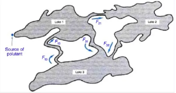
Figure 1. System of three lakes with interconnecting channels.
is obtained by
ci(t) = xi(t)
Vi .
Each lake initially is assumed to be free of any contaminant, soxi(0) = 0 fori= 1,2,3. To model the dynamic behavior of the system of lakes, we denote constantFjithe flow rate from lake, i to lake, j. These flow rates, which could be measured in gallons per minute or any other convenient units, are indicated in Fig. 1. Since there is no channel allowing any flow from lake 2 to lake 1, Note that F12 = 0. The flux of pollutant flowing from lake i into lake j at any time, writed byrji(t) , is defined by
rji(t) =Fjici(t) = Fji
Vi xi(t)
So rji(t) measures the rate at which the concentration of pollutant in lake i flows into lake j at time t. We will observe that
Rate of change of pollutant = Input rate −Output rate.
Using the above principle to each lake results in the following system of first order equations modelling the dynamic behavior of the lakes system:
dx1(t)
dt = F13
V3
x3(t) +p(t)−F31 V1
x1(t)−F21 V1
x1(t),
dx2(t) dt =
F21
V1 x1(t)− F32
V2 x2(t), 0≤t≤1
dx3(t)
dt = F31
V1
x1(t) +F32
V2
x2(t)−F13 V3
x3(t),
(1.1) with the initial conditions:
xi(0) = 0, i= 1,2,3. (1.2)
In order for the volume of each lake to remain constant, the flow rate into each lake must balance the flow out of the lake. Thus we assume the following conditions:
Lake 1: F13=F21+F31,
Lake 2: F21=F32,
Lake 3: F31+F32=F13.
In this paper, we approximate the solution of system (1.1) in terms of the truncated Ritz series as
xi(t)∼=xi,m(t) = m X
j=0
b?i,jtBj(t) | {z } φj(t)
= m X
j=0
b?i,jφj(t), i= 1,2,3, 0≤t≤1
where b?i,j (j = 0,1, ..., m) are unknown Ritz series coefficients and
Bj(t) (j = 0,1, ..., m) are the Bernoulli polynomials are introduced in section 2.
The organization of this paper is as follows:
In the next section, we introduce the basic Bernoulli polynomials and numbers and some their properties. In section 3, we present the appli-cation of Bernoulli Ritz-colloappli-cation method to the solution of modelling the pollution of a system of lakes. In section 4, we apply the Bernoulli Ritz-collocation method to a numerical example to demonstrate the ac-curacy of the present numerical method and the last section is included to conclusions.
2. Bernoulli polynomials and some their properties
Bernoulli polynomials play an important role in various expansions and approximation formulas which are useful both in analytic theory of numbers and in classical and numerical analysis. These polynomials can be defined by various methods depending on the applications [21, 22, 23, 24, 25].
The Bernoulli polynomials of i-th degree are defined on the interval [0,1] as
Bi(x) = i X
k=0
i k
Bkxi−k
where Bk := Bk(0) (k= 0,1, ..., i) are the Bernoulli numbers. Leopold Kronecker expressed the Bernoulli number Bi in the following form
Bi=− i+1
X
k=1
(−1)k
k
i+ 1
k
k
X
j=1
ji, i≥0, i6= 1.
Ifi= 1, we definedB1=−1
2. The Bernoulli polynomials and Bernoulli numbers are produced by the following generating functions, respec-tively,
text et−1 =
∞ X
n=0 Bn(x)
tn n! and
t et−1 =
∞ X
n=0 Bn
tn n!.
We have, in particular, B0 = 1, B1 = −1
2, B2 = 1
6, B3 = 0 , and
B2k+1 = 0, for k= 2,3, ...,
B0(x) = 1, B1(x) =x−1
2, B2(x) =x
2−x+1
6, B3(x) =x
3−3
2x
2+1
If, we define vectorCi+1,as
Ci+1=
ii
Bi i−i1
Bi−1 i−i2
Bi−2 . . . 1i
B1 0i
B0
m−i z }| { 0,0, ...,0
1×(m+1) ,
thenBi(t) =Ci+1 XT(t),for i=0, 1, ..., m, where
X(t) = [1t t2 ... tm].
Now, we can expand the matrixB(t) = [B0(t)B1(t)... Bm(t)] as
B(t) =X(t)CT, (2.1)
where C= C1 C2 C3 C4 .. .
Cm+1
=
B0 0 0 0 . . . 0
1 1
B1 10B0 0 0 . . . 0
2 2
B2 21
B1 20
B0 0 . . . 0
3 3
B3 32
B2 31
B1 30
B0 . . . 0
..
. ... ... ... . .. ...
m m
Bm mm−1
Bm−1 mm−2
Bm−2 mm−3
Bm−3 . . . m0
B0
(m+1)×(m+1) .
Also, if we define vectorDi+1, as
Di+1=
0 i−i1
Bi−1 2 i−i2
Bi−2 . . . (i−1) 1i
B1 i 0iB0
m−i z }| { 0,0, ...,0
1×(m+1) ,
thentdBi(t)
dt =Di+1X
T(t) for i=0, 1, ..., m, and we have
tdB(t)
dt =X(t)D
where D= D1 D2 D3 D4 .. .
Dm+1
=
0 0 0 0 . . . 0
0 10
B0 0 0 . . . 0
0 21B1 2 20B0 0 . . . 0
0 32B2 2 31B1 3 30B0 . . . 0
..
. ... ... ... . .. ...
0 mm−1Bm−1 2 mm−2
Bm−2 3 mm−3
Bm−3 . . . m m0
B0
(m+1)×(m+1) .
By using relations (2.1) and (2.2), we get
dφ(t)
dt =B(t) +t dB(t)
dt =T(t)C
T+T(t)DT =T(t)(CT +DT
| {z }
M
) =T(t)M,
(2.3) where
φ(t) =tB(t) = [tB0(t)tB1(t)... tBm(t)].
3. Bernoulli Ritz-collocation method
First, we can write the functions defined in relation (1.3) in the form
xi,m(t) =φ(t)Bi?, i= 1,2,3 (3.1) where
φ(t) = [tB0(t)tB1(t)... tBm(t)], Bi?= [b?i,0 b?i,1... bi,m? ]T, i= 1,2,3. Using the relations (2.3) and (3.1), we get recurrence relation
dxi,m(t) dt =
dφ(t)
dt B ?
i =T(x)M Bi?, i= 1,2,3 (3.2) By substituting the relations (3.1) and (3.2) in the system (1.1), we have
T(t)M B? 1 −
F13 V3 φ(t)B
? 3+
F31 V1 φ(t)B
? 1+
F21 V1 φ(t)B
?
1 =p(t),
T(t)M B2?−F21 V1
φ(t)B?1+F32
V2
φ(t)B2?= 0, 0≤t≤1
T(t)M B3?−F31 V1
φ(t)B?1−F32 V2
φ(t)B2?+ F13
V3
or briefly
h g
T(t)Mf+θφg(t) i
B? =α(t) (3.3)
where
g
T(t) =
T(t) 0 0 0 T(t) 0
0 0 T(t)
3×3 ,Mf=
M 0 0
0 M 0
0 0 M
, θ= F31 V1 + F21
V1 0 − F13
V3 −F21
V1
F32 V2
0
−F31 V1
−F32 V2 F13 V3
3×3 ,
g
φ(t) =
φ(t) 0 0 0 φ(t) 0
0 0 φ(t)
3×3
, α(t) =
p(t) 0 0
3×1 , β? =
β1? β? 2 β3?
3×1 .
Now, we substitute the collocaion points xs in relation (3.3) as h
]
T(ts)Mf+θφ](ts) i
B? =α(ts), s= 0,1, ..., m or briefly
h e
TMf+ Θφe i
B? =α (3.4)
where e T = ]
T(t0)
]
T(t1)
.. .
^
T(tm)
(m+1)×1 ,Θ =
θ 0 · · · 0 0 θ · · · 0
..
. ... . .. ... 0 0 · · · θ
(m+1)×(m+1) ,φe=
]
φ(t0)
]
φ(t1)
. ..
^
φ(tm)
and α=
α(t0) α(t1)
.. .
α(tm) .
The collocation points ts (s = 0,1, ..., m) are roots of the well-known shifted Chebyshev polynomials of order (m+1) on the interval [0, 1] and also can be chosen asts=
s
m, s= 0,1, ..., m.
We can write the system (3.4) in the formF B? =α, where F =TeMf+ Θφe. This system is an algebraic system of equations with 3×(m+ 1) equations and 3×(m+ 1) unknown coefficients, b?i,j for i= 1,2,3 and
j= 0,1, ..., m.
4. Error analysis and numerical example
We can easily check the convergence behavior of the Bernoulli Ritz-collocation method to the solution of the pollution of a system of lakes, by error functions ei,m(t) which come from putting the series solution xi,m(t) in system (1.1) defined by
e1,m(t) =
dx1,m(t) dt −
F13
V3 x3,m(t)−p(t) + F31
V1 x1,m(t) + F21
V1 x1,m(t)
e2,m(t) =
dx2,m(t) dt −
F21
V1 x1,m(t) + F32
V2 x2,m(t)
,
e3,m(t) =
dx3,m(t) dt −
F31 V1
x1,m(t)− F32
V2
x2,m(t) + F13
V3
x3,m(t)
.
If ei,m(t) −→ 0 (i= 1,2,3) when m is sufficiently large enough, then errors decrease.
In this section, the condition number of the matrix F,Kp(F), forp = 2,∞ is given by
Kp(F) =kF kpkF
−1 k
p, p= 2,∞.
The condition numberKp(F) shows that a small perturbation in initial data may produce a large amount of perturbation in the solution. Also, the CPU time used for solving algebraic system of equations (3.4) is given for the following example.
4.1. Example. Consider the following system of equations [16]
dx1(t) dt =
38
1180x3(t) +{1 +sin(t)} − 20
2900x1(t)− 18 2900x1(t),
dx2(t) dt =
18
2900x1(t)− 18 850x2(t),
dx3(t) dt =
20
2900x1(t) + 18
850x2(t)− 38 1180x3(t),
(4.1) with the initial conditions:
xi(0) = 0, i= 1,2,3.
Also, in this example p(t) = 1 +sin(t) and the parameter values have been fixed to V1 = 2900 mi3, V2 = 850 mi3, V3 = 1180 mi3, F21 = 18mi3/year,F32 = 18mi3/year,F31 = 20mi3/year,F13 = 38mi3/year. We solve the system of equations (4.1) by the Bernoulli Ritzr-collocation method. The approximate solutions xi,m (i = 1,2,3) of this system of equations are obtained for m= 4,7,9, respectively,
x1,4(t) = (0.40465058683e−002)t5−(0.458432145597e−001)t4−(0.150994938452e−003)t3
+0.493097145228t2+ 1.0t,
x1,7(t) =−(0.214732591743e−004)t8−(0.107307557937e−004)t7+(0.139751725613e−002)t6
+(0.103363484193e−003)t5−(0.416486605518e−001)t4−(0.211867369508e−002)t3
+0.493448309148t2+ 1.0t,
−(0.416507239823e−001)t4−(0.211827495596e−002)t3+0.493448275806t2+1.0t, x2,4(t) =−(0.438030487978e−004)t5−(0.197980651106e−004)t4+(0.100508516316e−002)t3
+(0.310222747099e−002)t2−(2.42499786143e−018)t,
x2,7(t) =−(0.777494864254e−007)t8+(0.136225929849e−005)t7+(0.163646619054e−006)t6 −(0.515911297141e−004)t5−(0.860226992733e−005)t4+(0.99902571917e−003)t3
+(0.310344787306e−002)t2−(2.08301041702e−017)t,
x2,9(t) = (0.865676197392e−009)t10−(0.189583709547e−007)t9−(0.277212664629e−008)t8
+(0.122804942835e−005)t7+(0.296374287309e−006)t6−(0.516684248401e−004)t5 −(0.857582185107e−005)t4+ (0.99902076182e−003)t3
+(0.310344827652e−002)t2+ (2.18771356907e−017)t,
x3,4(t) =−(0.489122665739e−004)t5−(0.196193971649e−004)t4+(0.112588977284e−002)t3
+(0.344693737064e−002)t2+ (1.22876358446e−018)t,
x3,7(t) =−(0.852391271317e−007)t8+(0.151487170973e−005)t7+(0.104552072488e−006)t6 −(0.573522953422e−004)t5−(0.740363586521e−005)t4+(0.111926067663e−002)t3
+(0.344827541228e−002)t2+ (1.71593075047e−017)t,
and
x3,9(t) = (0.948960812708e−009)t10−(0.210817400585e−007)t9−(0.170076132344e−008)t8
+(0.136521931168e−005)t7+(0.252616368201e−006)t6−(0.574385464347e−004)t5 −(0.737411698542e−005)t4+ (0.111925514251e−002)t3
+(0.344827586284e−002)t2+ (4.6305965127e−016)t.
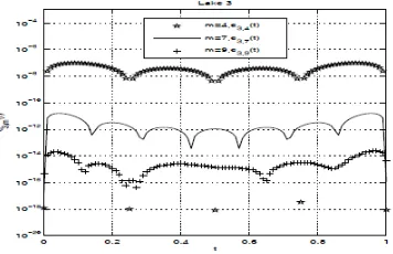
Tables 1, 2 and 3 show the approximate solutionsx1,m(t), x2,m(t)x3,m(t) and error functionse1,m(t), e2,m(t),
e3,m(t), for m = 4,7,9, respectively, of lake 1, 2 and 3. The condition number Kp(F) of p = 2,∞ and CP U time at various value of m of system (4.1) are shown in Table 4. Figs. 2, 3 and 4 give us the com-parison of the error functionse1,m(t), e2,m(t), e3,m(t) form= 4,7,9 and 0≤t≤1, respectively, of lake 1, 2 and 3.
Table 1: Approximate solutions x1,m(t) and the error
functions e1,m(t), for m= 4,7,9, of lake 1.
ti m= 4, x1,4(ti) m= 4, e1,4(ti) m= 7, x1,7(ti) m= 7, e1,7(ti) m= 9, x1,9(ti) m= 9, e1,9(ti)
0.0 0.0000000 0.0000e−000 0.0000000 0.0000e−000 0.0000000 0.0000e−000 0.2 0.2196506 9.7510e−006 0.2196545 2.5589e−010 0.2196545 3.7269e−013 0.4 0.4777637 9.1587e−006 0.4777567 5.8930e−011 0.4777567 4.6978e−013 0.6 0.7715570 8.9919e−006 0.7718587 6.1398e−011 0.7718587 8.0520e−013 0.8 1.0980530 9.2274e−006 1.0980570 2.8829e−010 1.0980570 5.2182e−013 1.0 1.4511490 3.7076e−015 1.4511500 1.3810e−013 1.4511500 1.6909e−012
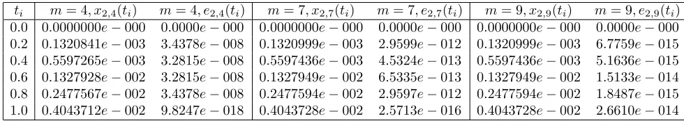
Table 2: Approximate solutions x2,m(t) and the error
ti m= 4, x2,4(ti) m= 4, e2,4(ti) m= 7, x2,7(ti) m= 7, e2,7(ti) m= 9, x2,9(ti) m= 9, e2,9(ti)
0.0 0.0000000e−000 0.0000e−000 0.0000000e−000 0.0000e−000 0.0000000e−000 0.0000e−000 0.2 0.1320841e−003 3.4378e−008 0.1320999e−003 2.9599e−012 0.1320999e−003 6.7759e−015 0.4 0.5597265e−003 3.2815e−008 0.5597436e−003 4.5324e−013 0.5597436e−003 5.1636e−015 0.6 0.1327928e−002 3.2815e−008 0.1327949e−002 6.5335e−013 0.1327949e−002 1.5133e−014 0.8 0.2477567e−002 3.4378e−008 0.2477594e−002 2.9597e−012 0.2477594e−002 1.8487e−015 1.0 0.4043712e−002 9.8247e−018 0.4043728e−002 2.5713e−016 0.4043728e−002 2.6610e−014
Table 3: Approximate solutions x3,m(t) and the error
functions e3,m(t), for m= 4,7,9, of lake 3.
ti m= 4, x3,4(ti) m= 4, e3,4(ti) m= 7, x3,7(ti) m= 7, e3,7(ti) m= 9, x3,9(ti) m= 9, e3,9(ti)
0.0 0.0000000e−000 0.0000e−000 0.0000000e−000 0.0000e−000 0.0000000e−000 0.0000e−000 0.2 0.1468376e−003 3.7692e−008 0.1468549e−003 3.3052e−012 0.1468549e−003 1.1916e−015 0.4 0.6225638e−003 3.5979e−008 0.6225828e−003 7.2953e−013 0.6225828e−003 2.4982e−015 0.6 0.1477744e−002 3.5979e−008 0.1477766e−002 7.2954e−013 0.1477766e−002 1.0118e−015 0.8 0.2758432e−002 3.7692e−008 0.2758463e−002 3.3051e−012 0.2758463e−002 2.4024e−015 1.0 0.4504295e−002 8.5833e−019 0.4504314e−002 1.1749e−016 0.4504314e−002 4.5485e−015
Table 4: Condition number Kp(F) of p= 2,∞ and CP U time at
various value of m of system (4.1).
m= 4 m= 7 m= 8 m= 9
K2(F) 5.9706e+ 001 8.0873e+ 003 4.8105e+ 004 2.9455e+ 005 K∞(F) 1.4708e+ 002 1.7999e+ 004 1.1239e+ 005 7.2357e+ 005
CP U time(s) 2.75 2.85 3.82 4.29
5. conclution
Figure 2. Comparison of the error functions e1,m for m= 4,7,9 and 0≤t≤1 of lake 1.
Figure 3. Comparison of the error functions e2,m for m= 4,7,9 and 0≤t≤1 of lake 2.
Figure 4. Comparison of the error functions e3,m for m= 4,7,9 and 0≤t≤1 of lake 3.
References
[2] M. Javidi, Iterative methods to nonlinear equations , Applied Mathematics and Computation. 193 (2007) 360–365.
[3] S. A. Yousefi, A. Banifatemi, Numerical solution of Fredholm integral equa-tions by using CAS wavelets, Applied Mathematics and Computation. 183 (2006) 458–463.
[4] K. Maleknejad, M. Attary, An efficient numerical approximation for the linear class of Fredholm integro-differential equations based on Cattani’s method, Commun Nonlinear Sci Numer Simulat. 16 (2011) 2672–2679. [5] A. Makroglou, Convergence of a Block-By-Block Method for Nonlinear
Volterra Integro-Differential Equations, Mathematics of Computation. 35 (151) (1980) 783–796.
[6] K. Sty´s , T. Sty´s, A higher-order finite difference method for solving a sys-tem of integro-differential equations, Journal of Computational and Ap-plied Mathematics. 126 (2000) 33–46.
[7] K. Maleknejad, B. Basirat, E. Hashemizadeh, Hybrid Legendre polynomi-als and Block-Pulse functions approach for nonlinear Volterra–Fredholm integro-differential equations, Computers and Mathematics with Applica-tions. 61 (2011) 2821–2828.
[8] M. Lakestani, B. Nemati Saray, M. Dehghanb, Numerical solution for the weakly singular Fredholm integro-differential equations using Legendre multiwavelets, Journal of Computational and Applied Mathematics. 235 (2011) 3291–3303.
[9] M. Sezer, A. Karamete, M. G¨ulsu, Taylor polynomial solutions of systems of linear differential equations with variable coefficients, International Jour-nal of Computer Mathematics. 82 (6) (2005) 755–764.
[10] M. G¨ulsu, M. Sezer, Approximations to the solution of linear Fred-holm integrodifferential–difference equation of high order , Journal of the Franklin Institute. 343 (2006) 720–737.
[11] A. Aky¨uz-Da¸scıo˘glu, A Chebyshev polynomial approach for linear Fredholm–Volterra integro-differential equations in the most general form, Applied Mathematics and Computation. 181 (2006) 103–112.
[12] S. Yal¸cinba¸s, M. Sezer, H. H. Sorkun, Legendre polynomial solutions of high-order linear Fredholm integro-differential equations, Applied Mathe-matics and Computation. 210 (2009) 334–349.
[13] S¸. Y¨uzba¸sı, N. S¸ahin, M. Sezer, Bessel polynomial solutions of high-order linear Volterra integro-differential equations, Computers and Mathematics with Applications. 62 (4) (2011) 1940–1956.
[14] E. Sokhanvar, S. A. Yousefi, The Bernoulli matrix method for solving a family of integro-differential equations with weakly singular kernel, Journal of Advanced Research in Scientific Computing. 4 (4) (2012) 18–32. [15] E. Sokhanvar, S. A. Yousefi, An effective method for numerical solution of
delay differential equations of multi-pantograph type, Journal of Advanced Research in Dynamical and Control Systems. 5 (4) (2013) 20–36.
[17] J. Biazar, M. Shahbala, H. Ebrahimi, VIM for solving the pol-lution problem of a system of lakes, J. Control Sci. Eng. (2010). doi:10.1155/2010/829152.
[18] M. Merdan, Homotopy perturbation method for solving modelling the pol-lution of a system of lakes, SDU JOURNAL OF SCIENCE (E-JOURNAL). 4 (1) (2009) 99–111.
[19] S¸uayip Y¨uzba¸sı,N. S¸ahin, M. Sezer, A collocation approach to solving the model of pollution for a system of lakes, Mathematical and Computer Modelling. 55 (2012) 330–341.
[20] M. Merdan, A New Application of Modified Differential Transformation Method for Modelling the Pollution of a System of Lakes, Sel¸cuk J. Appl. Math. 11 (2) (2010) 27–40.
[21] F. Costabile, F. Dell’accio, M. I. Gualtieri, A new approach to Bernoulli polynomials, Rendiconti di Matematica. 26 (2006) 1–12.
[22] P. Natalini, A. Bernardini, A generalization of the Bernoulli polynomials, J. Appl. Math. 3 (2003) 155–163.
[23] T. Agoh, K. Dilcher, Integrals of products of Bernoulli polynomials, J. Math. Anal. Appl. 381 (2011) 10–16.
[24] B. Kurt, Y. Simsek, Notes on generalization of the Bernoulli type polyno-mials, Appl. Math. Comput. 218 (2011) 906–911.