New Randomized Response Procedures

New Randomized Response Procedures

Z. Hussain

1,2,*

and J. Shabbir

2

1_{Department of Statistics, Faculty of Sciences, King Abdulaziz University 80203, Jeddah 21589, Saudi Arabia} 2_{Department of Statistics, Faculty of Sciences, Quaid-i-Azam University 45320, Islamabad 44000, Pakistan}

Received: 16 January 2012 / Revised: 3 December 2012 / Accepted: 7 January 2013

Abstract

This article focuses on the estimation of population proportion when the study

variable is sensitive in nature. Two implicit randomized response techniques are

proposed where the unrelated trait can be chosen subjectively. In addition to

unbiased estimation of population proportion and variance, an empirical study is

conducted to inspect the relative efficiency facet of the proposed techniques. The

cases of positive binomial and negative binomial sampling are also studied. The

proposed techniques are exposed to be better at the job than the accustomed

randomized response dealings in binomial sampling. Further, it is established that

negative binomial sampling may result in more precise estimation of population

proportion using the proposed techniques.

Keywords: Randomized response; Estimation of proportion; Sensitive attribute; Dichotomous

population and Relative efficiency

* _{Corresponding author, Tel.: +92(51)90642185, E-mail: [email protected]} Introduction

Survey techniques are applied more or less in every field of scientific and social studies ranging from physical sciences to economics, from business studies to bioinformatics, from educational behaviors to reliability engineering etc. Collection of unswerving information has come out as an exigent concern in socio-economic and behavioral studies reason being making dependable and compelling inferences primarily depends upon the dependability of the data. Warner [32], for the first time considered this concern and projected an inventive and original technique, called Randomized Response Technique (RRT), to elicit truthful data for estimating proportion of a sensitive trait. Warner’s method consists of two randomized questions pertaining to the possession of a sensitive attribute A or its non-sensitive complement A . The idea of randomizing the response

direct questions about the possession of a sensitive trait. In the forced response model some respondents may feel embarrassed to report simply a yes response. In the unrelated question randomized response models there is a requirement of two independent sub-samples and optimal allocation of sample size into two sub-samples depends upon the unknown value of . Further, the relative efficiency is related to the values of Y as it requires to have _Y on the same side of 0.5 as is the .

The maximum efficiency is achieved when _Y 0.5 is maximum. In practice, it is difficult to have such an unrelated attribute Y for which _Y 0.5 is a maximum. Also, because  is unknown, the selection of unrelated attribute becomes more difficult.

In many practical situations, generally, multiple sensitive items are studied. It may happen that some of the items are very rare (abundant) with very small (large) population proportions. For such items the probability of a yes response through a given RRT turns out to be very small (large). Obviously, in these situations we may have a small (large) number of yes responses which is not desirable from privacy point of view. For example, in a psychological/medical study the number of patients who evade tax may be very small. In such cases the probability of having an estimate outside the [0,1] interval is increased. To avoid such cases, Mangatand Singh [21] suggested applying negative binomial sampling with Warner [32] RRT. Singh and Mathur [29] extended the study by Mangat and Singh [21] and suggested several upper bounds on the variance of the estimator. The application of negative binomial sampling to unrelated trait RRTs cannot be found in literature. Moreover, through many studies, it has been established that unrelated trait RRTs perform relatively better (see Greenberg et al. [10], Mahmood et al. [19], and Huang [14], etc.). Therefore, the problem of studying the unrelated trait RRTs becomes more apparent and demanding. In this paper, we study the unrelated trait RRTs and improve them further by using negative binomial sampling.

The contribution of this paper is twofold in the sense that we suggest two new unrelated trait RRTs and study their performance under binomial and negative binomial sampling methods. There are two adavantages of the proposed RRTs: we do not need the two subsamples, and the unrelated trait may be chosen arbitrarly. Also, the proposed randomized response procedures circumvent the difficulties pointed out by Huang [14]. Iin addition, proposed estimators yeild a moderate number of yes responses to maintain privacy and consequently obtaining an estimate in the interval [0,1].

Further, three upper bounds of the variances of the proposed estimators are also given and compared with each other along with the exact variance. The proposed techniques are studied using binomial sampling and compared with that of Mangat et al. [21], Mahmood et al. [19] and Bhargava and Singh [4] randomized response techniques. The proposed techniques are also studied using negative binomial sampling and then comparison of positive and negative binomial sampling methods is made for some values of the design parameters.

The organization of the paper is as follows. In sections 2 and 3, we present the proposed techniques assuming binomial and negative binomial sampling designs. Comparisons are made in section 4 followed by conclusion in section 5.

The Proposed Techniques Assuming Binomial Sampling

This section presents two new techniques for estimating the population proportion of a sensitive attribute.

Technique I

Consider a dichotomous population U =



u u1, 2,...,uN



in which every ui can be classified either to a sensitive group A or to its compliment, A . The focus of the study lies in the estimation of the population proportion of the u s_i' which are actually classified in the sensitive group A. Let Y be an unrelated trait. In the proposed technique a simple random sample of size n is drawn with replacement from the population. The proposed procedure consists of two types of statements. With probability p1 the respondent is asked to answer to the statement (a) “I possess both the attributes A and Y ” and with probability



1p1



to answer (b) “I posses the attribute

A and do not possess the attribute Y ”. The statement randomly selected by the interviewee is unseen to the surveyor. Let P

 

. be the probability of a particular

eventthen P A

 

 . Through the suggested technique, the probability of obtaining a yes answer is given by





















1 1 1 1

c

p P A Y p P A Y

     



   

 







1 1 p P A1 2p1 1 P A Y

      . (1)

Now form (1) it is obvious that to have probability of





P A Y must be zero, which will be the case when

1 0.5

p  . Consequently, we have

1 1 2

  . (2)

Using (2) and method of moments, an unbiased estimator of  is proposed as

1 ˆ1

ˆ 2

   , (3)

Where 1

1

ˆ n

n

  and n1 is the number of yes responses

in the sample.

The variance of ˆ1 is given by

 

1



1



1 4 1 ˆ V ar n  

   . (4)

Substituting the value of

 

1 from (2) in (4) we get

 

1









4 1

2 1

2 2

ˆ V ar

n n n n

          _     _{ }   

    , (5)

which is unbiasedly estimated by

 

1



1



1 ˆ ˆ 4 1 ˆ _ˆ 1 V ar n     

 . (6)

Technique II

The second technique works in a similar manner as the first one except a minor difference in the statements. The statements, in the Technique II are: (c) “I Possess the attribute Y and do not possess the attribute A” and (d) “ I do not possess both the attributes A and Y ”. The rest of the things in Techniques I and II are identical. Now, the probability of a yes answer is given by





















2 2 1 2

c c c

p P A Y p P A Y

     







 















2 1 2 1 2 2 1

c

p P A p P A Y

       .(7)

As in the Technique I, to have 2 unconnected to

the attribute Y , the coefficient of P A



cY



must be

zero, which is the case when p₂ 0.5. As a consequence 2 is given by







 



2 1 p2 1 P A

    =

 

0.5 1



. (8)

From (8), we have

2 0.5

0.5



   . (9)

Thus using (9) and moment method of estimation, we have an unbiased estimator of the population proportion given by

2 2 ˆ 0.5 ˆ 0.5 

   , (10)

with variance, given by

 

2



2





 



2

4 1 1 1

ˆ V ar

n n n

    

       . (11)

An unbiased estimator of Var

 

ˆ2 is given by

 

2



2



2 ˆ ˆ 4 1 ˆ _ˆ 1 Var n     

 . (12)

Proposed Techniques Assuming Negative Binomial Sampling

From (2) it is obvious that when the population proportion  is very small (which may be the case in most of practical situations) the value of 1 will be small and 2 will be large. For such cases, the number of yes responses in the sample will be small for not so large n. However, having a small number of yes responses may not be desirable from practical point of view. In order to avoid this we may use negative binomial sampling where sampling is continued until a fixed number m of yes responses are obtained. Here the sample size n is not fixed in advance. By considering the two techniques discussed above, using negative binomial sampling, unbiased estimators of  are defined as given in (2) and (10) but here

1

ˆ _{, 1, 2.} 1

j

m _j

n

   

 To derive the variance of these

two estimators under negative binomial sampling we use the following lemma as given in the Best [2].

Lemma 3.1: If ˆ ~Negative Binomial m



,



then

 







 





 

2 1 2

ˆ _{1 1}

1

1 log .

1 1

t t m

m m e t E m m t     _                 _  _     _   _   _    



 (13)

 











 



 

1 2 2 ˆ

4 1 1 1

1

1 log .

1 j t t m j j t j m m j

e j j

j Var m m t             _{    }    _{ } _{   }    _  _  _{ }         _    _ _       _{ }



(14)

It is to be noted that for the existence of variance expression in (14) we must fix m 2. It is obvious from (14) that as m increases it becomes tedious to have a numerical value of the variances through (14). However, following Sathe [27], Pathak and Sathe [25] and Sahai [26] different upper bound of the variances in (14) can be found.

Sathe [27] reported following upper bound for the variance of negative binomial estimator

 





















1 2 2 ˆ 2 1 .

2 1 2 1 4 1

UBV m m                 (15)

Sahai [26] derived the upper bound for variance of the negative binomial estimator as given by

 

2

2 ˆ 12

6

UBV A m B A

m 

  _    _, (16)

where











2 _{3 1 3 1}



6 1









2

1

A m m

m      _              and







11

 

1

 

2

 

1



m

B m

m  

     _    _       .

The upper bound for the variance due to Pathak and Sathe [25] is given by

 

2













3

1 2 1

ˆ ₁ 2 UBV m m       _    







 

 





₂







0.5

12 1

2 3 2 5 4 16 1

m m m

            _  _        _   .(17)

Thus using (15), (16) and (17) in (14) the different

upper bounds of the variance of unbiased estimators of

π obtained through Techniques 1 and 2 are now given by

 





















1 2 2 ˆ 8 1

2 1 2 1 4 1

j

j j

j j j j

UBV m m                 , (18)

 

2

2

4

ˆ 12

6 j

j j j j j

UBV A m B A

m



  _    _, (19)

where Aj and Bj ,



j 1, 2



are defined as earlier, and

 

2













3

4 1 2 1

ˆ 1

2

j j j

j UBV m m           











 





₂







0.5

12 1

2 3 2 5 4 16 1

j j

j j j j

m m m

         _      _        _   .(20)

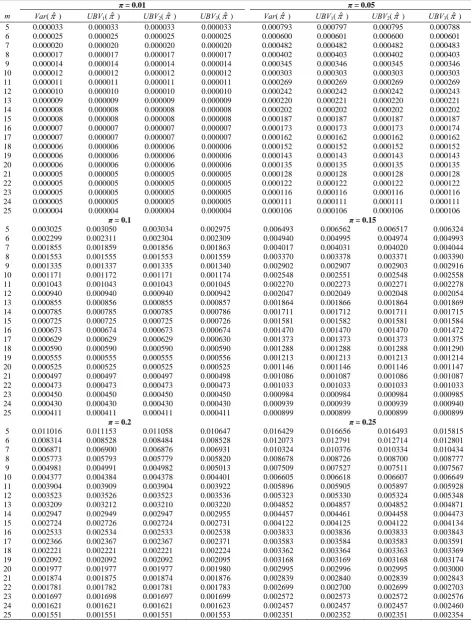
It is to be mentioned that the values of the exact variance of the estimator ˆ2 and its different upper bounds are calculated numerically for different values of  and are given in the Table 1 (similarly, the upper bounds on the variance of ˆ1 can be calculated). From Table 1, it is observed that for  0.01 and 0.05, all the three upperbounds UBV1

 

ˆ2 , UBV2

 

ˆ2 and

 

3 ˆ2

UBV  are exactly equal to the actual variance ,

 

ˆ2

Var  , over a wide range of m . For  0.1, and 12

m  , UBV1

 

ˆ2 and UBV2

 

ˆ2 are equal to the

actual variance followed by UBV1

 

ˆ2 . For  0.1 and 12m 25 all the three upperbounds are equal to actual variances. When  0.15 and m 25 all the upperbounds are equal to true variance. When

5m25, UBV2

 

ˆ2 is closer to the true variance followed by UBV1

 

ˆ2 and UBV3

 

ˆ2 . Similarly

when  0.2, 0.25, UBV2

 

ˆ2 is closer to the true variance followed by UBV1

 

ˆ2 and UBV3

 

ˆ2 . From the above observation a general conclusion can be made that for 0.01  0.25 and 5m25, UBV2

 

ˆ2 is the best approximation of the Var

 

ˆ2 compared to

 

1 ˆ2

UBV  and UBV₃

 

ˆ₂ . Therefore, to calculate the

Table 1. Values of exact variance of ˆ2 under negative binomial sampling and its upper bounds for different values of  and m

π = 0.01 π = 0.05

m Var(ˆ) UBV1(ˆ) UBV2(ˆ) UBV3(ˆ) Var(ˆ) UBV1(ˆ) UBV2(ˆ) UBV3(ˆ)

5 0.000033 0.000033 0.000033 0.000033 0.000793 0.000797 0.000795 0.000788 6 0.000025 0.000025 0.000025 0.000025 0.000600 0.000601 0.000600 0.000601 7 0.000020 0.000020 0.000020 0.000020 0.000482 0.000482 0.000482 0.000483 8 0.000017 0.000017 0.000017 0.000017 0.000402 0.000403 0.000402 0.000403 9 0.000014 0.000014 0.000014 0.000014 0.000345 0.000346 0.000345 0.000346 10 0.000012 0.000012 0.000012 0.000012 0.000303 0.000303 0.000303 0.000303 11 0.000011 0.000011 0.000011 0.000011 0.000269 0.000269 0.000269 0.000269 12 0.000010 0.000010 0.000010 0.000010 0.000242 0.000242 0.000242 0.000243 13 0.000009 0.000009 0.000009 0.000009 0.000220 0.000221 0.000220 0.000221 14 0.000008 0.000008 0.000008 0.000008 0.000202 0.000202 0.000202 0.000202 15 0.000008 0.000008 0.000008 0.000008 0.000187 0.000187 0.000187 0.000187 16 0.000007 0.000007 0.000007 0.000007 0.000173 0.000173 0.000173 0.000174 17 0.000007 0.000007 0.000007 0.000007 0.000162 0.000162 0.000162 0.000162 18 0.000006 0.000006 0.000006 0.000006 0.000152 0.000152 0.000152 0.000152 19 0.000006 0.000006 0.000006 0.000006 0.000143 0.000143 0.000143 0.000143 20 0.000006 0.000006 0.000006 0.000006 0.000135 0.000135 0.000135 0.000135 21 0.000005 0.000005 0.000005 0.000005 0.000128 0.000128 0.000128 0.000128 22 0.000005 0.000005 0.000005 0.000005 0.000122 0.000122 0.000122 0.000122 23 0.000005 0.000005 0.000005 0.000005 0.000116 0.000116 0.000116 0.000116 24 0.000005 0.000005 0.000005 0.000005 0.000111 0.000111 0.000111 0.000111 25 0.000004 0.000004 0.000004 0.000004 0.000106 0.000106 0.000106 0.000106

π = 0.1 π = 0.15

5 0.003025 0.003050 0.003034 0.002975 0.006493 0.006562 0.006517 0.006324 6 0.002299 0.002311 0.002304 0.002309 0.004940 0.004995 0.004974 0.004993 7 0.001855 0.001859 0.001856 0.001863 0.004017 0.004031 0.004020 0.004044 8 0.001553 0.001555 0.001553 0.001559 0.003370 0.003378 0.003371 0.003390 9 0.001335 0.001337 0.001335 0.001340 0.002902 0.002907 0.002903 0.002916 10 0.001171 0.001172 0.001171 0.001174 0.002548 0.002551 0.002548 0.002558 11 0.001043 0.001043 0.001043 0.001045 0.002270 0.002273 0.002271 0.002278 12 0.000940 0.000940 0.000940 0.000942 0.002047 0.002049 0.002048 0.002054 13 0.000855 0.000856 0.000855 0.000857 0.001864 0.001866 0.001864 0.001869 14 0.000785 0.000785 0.000785 0.000786 0.001711 0.001712 0.001711 0.001715 15 0.000725 0.000725 0.000725 0.000726 0.001581 0.001582 0.001581 0.001584 16 0.000673 0.000674 0.000673 0.000674 0.001470 0.001470 0.001470 0.001472 17 0.000629 0.000629 0.000629 0.000630 0.001373 0.001373 0.001373 0.001375 18 0.000590 0.000590 0.000590 0.000590 0.001288 0.001288 0.001288 0.001290 19 0.000555 0.000555 0.000555 0.000556 0.001213 0.001213 0.001213 0.001214 20 0.000525 0.000525 0.000525 0.000525 0.001146 0.001146 0.001146 0.001147 21 0.000497 0.000497 0.000497 0.000498 0.001086 0.001087 0.001086 0.001087 22 0.000473 0.000473 0.000473 0.000473 0.001033 0.001033 0.001033 0.001033 23 0.000450 0.000450 0.000450 0.000450 0.000984 0.000984 0.000984 0.000985 24 0.000430 0.000430 0.000430 0.000430 0.000939 0.000939 0.000939 0.000940 25 0.000411 0.000411 0.000411 0.000411 0.000899 0.000899 0.000899 0.000899

π = 0.2 π = 0.25

Now we study the relative efficiency features of the proposed techniques relative to some usual randomized response techniques.

Efficiency Comparisons and Discussion

We, now, compare the proposed RRTs under the two cases of sampling, namely, binomial and negative binomial sampling.

(a) Case of Binomial Sampling (i) ˆ₁ versus ˆ₂

The proposed estimator ˆ1 will be relatively more efficient than the second proposed estimator ˆ₂ if

 

ˆ1

 

ˆ2

Var  Var  . (21)

Using (5) and (11) in (21) we see that the inequality (21) holds when  0.5, which implies that the ˆ1 will be more precise as compared to ˆ2 for  0.5. On the other hand, ˆ2 will be more efficient than ˆ1 when

0.5

  . It is quite clear that the two estimators ˆ1 and

2 ˆ

 will be equally good at  0.5.

(ii) Proposed estimators (ˆ1 and ˆ2) versus

Mahmood et al. estimator

We compare our proposed estimators ˆ1 and ˆ2 with the Mahmood et al. [19] estimator depending upon the value of the population proportion . Mahmood et al. [19] actually presented three estimators and indicated one as the best of them. We take this best one for our comparison purposes. The minimum variance expression of the Mahmood et al. [19] estimator , say

3 ˆ

 , is given by

 









3 min

2

3 3 2 3

2 1 ˆ

1 1

,

Y Y

V ar

p p

np 

   



 _{   } 

  (22)

where 3 p1p2



1Y



p3Y , and p1, p2, p3 are pre-assigned probabilities of randomly selecting the statements concerning the possession of A, Y c, and Y , respectively. An empirical study is undertaken to see the variation in extent of relative efficiency by fixing the practicable values of the parameters. The Relative Efficiency (RE) of the proposed estimators with respect to Mahmood et al. [19] procedure is defined as

 

 

 

 

3 min

2

1

3 min

1 ˆ

, if 0.5 ˆ

ˆ

, if 0.5. ˆ

Var Var RE

Var V ar



 



 



 

   

 



We have chosen p₁0.5 and values of p₃ are taken as i 



1 p1



9, i 1, 2, 3, 4 against the whole

range of . It is observed that for





3 1 1 9, 5, 6, 7,8

p   i p i  the values of RE1 are the mirror image of the values when i 1, 2, 3, 4. Therefore, for the sake of brevity, we have not provided the values of RE1 for i 1, 2, 3, 4. The values of RE1 are presented in Table 2 which clearly shows the better performance of the proposed estimators as compared to the Mahmood et al. [19] procedure. It is observed that for a fixed value of _Y the RE1 decreases when

0.5

 increases. Also, RE1 increases, for fixed values of _Y and , if p₃0.5 increases. The

magnitude of RE1 ranges from 1.42 to 9.25.

(iii) Proposed estimators versus Mangat et al. and Bhargava and Singh estimators

The variance expression of Mangat et al. [23] estimator, say ˆ4, is given by

 















2 2



3

4 2

1 2 1 2

1 1

ˆ p p p

Var

n n p p _{n p p}

  

     

  , (23)

where p1 and p2 are the pre-assigned probabilities of choosing a question concerning the membership in A,

c

A and p3 proportion of the sampled respondents are requested to say just no. The variance of Bhargava and Singh [4] estimator, say ˆ5, is given by

 















1 1



3

5 2

1 2 1 2

1 1

ˆ p p p

Var

n n p p _{n p p}

  

     

  , (24)

where p1 and p2 are same as that of Mangat et al. [23] procedure, and p3 is the probability of reporting just a

yes answer.

It has been reported by Bhargava and Singh [4] that their estimator is better than Mangat et al. [23] estimator if  0.5. So we have defined the RE of our proposed estimators depending upon the values of the . When

0.5

Table 2. The values of RE1 of the estimators ˆ1 and ˆ2 with respect to ˆ3

Y

 

0.1 0.2 0.3 0.4 0.5 0.6 0.7 0.8 0.9 p

3 = 1/8

0.1 7.95 4.22 2.95 2.29 1.86 2.04 2.34 2.91 4.61

0.3 9.25 5.03 3.60 2.86 2.40 2.73 3.26 4.31 7.42

0.5 8.96 5.00 3.67 2.99 2.57 2.99 3.67 5.00 8.96

0.7 7.42 4.31 3.26 2.73 2.40 2.86 3.60 5.03 9.25

0.9 4.61 2.91 2.34 2.04 1.86 2.29 2.95 4.22 7.95

p₃ = 2/8

0.1 6.96 3.76 2.66 2.09 1.73 1.93 2.25 2.88 4.74

0.3 7.73 4.24 3.06 2.45 2.07 2.37 2.84 3.77 6.53

0.5 7.50 4.21 3.10 2.53 2.17 2.53 3.10 4.21 7.50

0.7 6.53 3.77 2.84 2.37 2.07 2.45 3.06 4.24 7.73

0.9 4.74 2.88 2.25 1.93 1.73 2.09 2.66 3.76 6.96

p₃ = 3/8

0.1 5.95 3.27 2.36 1.88 1.58 1.79 2.13 2.78 4.70

0.3 6.31 3.51 2.56 2.07 1.76 2.02 2.44 3.25 5.66

0.5 6.17 3.48 2.57 2.10 1.81 2.10 2.57 3.48 6.17

0.7 5.66 3.25 2.44 2.02 1.76 2.07 2.56 3.51 6.31

0.9 4.70 2.78 2.13 1.79 1.58 1.88 2.36 3.27 5.95

p₃ = 4/8

0.1 4.93 2.77 2.04 1.66 1.42 1.63 1.97 2.62 4.54

0.3 5.02 2.84 2.10 1.71 1.47 1.70 2.06 2.76 4.82

0.5 4.97 2.83 2.10 1.72 1.48 1.72 2.10 2.83 4.97

0.7 4.82 2.76 2.06 1.70 1.47 1.71 2.10 2.84 5.02

0.9 4.54 2.62 1.97 1.63 1.42 1.66 2.04 2.77 4.93

Table 3. The values of RE2 of the estimators ˆ1 and ˆ2 with respect to ˆ4 and ˆ5

p₃ 

0.1 0.2 0.3 0.4 0.5 0.6 0.7 0.8 0.9

1/18 81.80 84.33 88.91 96.23 107.66 96.23 88.91 84.33 81.80

2/18 20.44 21.05 22.15 23.91 26.66 23.91 22.15 21.05 20.44

3/18 9.08 9.33 9.79 10.52 11.66 10.52 9.79 9.33 9.08

4/18 5.10 5.23 5.46 5.83 6.41 5.83 5.46 5.23 5.10

5/18 3.26 3.33 3.46 3.66 3.98 3.66 3.46 3.33 3.26

6/18 2.26 2.30 2.37 2.48 2.66 2.48 2.37 2.30 2.26

7/18 1.66 1.68 1.71 1.77 1.87 1.77 1.71 1.68 1.66

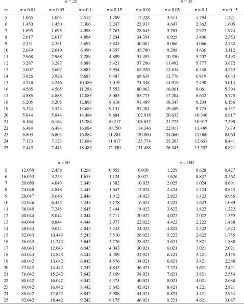
Table 4. The values of RE of proposed estimator ˆ2 under negative binomial sampling relative to binomial sampling for different

values of n, π and m

n = 25 n = 35

m π = 0.01 π = 0.05 π = 0.1 π = 0.15 π = 0.01 π = 0.05 π = 0.1 π = 0.15 5 1.065 1.065 2.512 1.709 17.228 3.511 1.794 1.221 6 1.450 1.450 3.306 2.247 22.933 4.647 2.362 1.605 7 1.695 1.695 4.098 2.763 28.643 5.785 2.927 1.974 8 2.017 2.017 4.894 3.294 34.354 6.925 3.496 2.353 9 2.331 2.331 5.692 3.825 40.067 8.066 4.066 2.732 10 2.649 2.649 6.490 4.357 45.780 9.208 4.636 3.112 11 2.968 2.968 7.289 4.889 51.493 10.350 5.207 3.492 12 3.287 3.287 8.088 5.421 57.206 11.492 5.777 3.872 13 3.607 3.607 8.887 5.954 62.920 12.634 6.348 4.253 14 3.926 3.926 9.687 6.487 68.634 13.776 6.919 4.633 15 4.246 4.246 10.486 7.019 74.348 14.919 7.490 5.014 16 4.565 4.565 11.286 7.552 80.062 16.061 8.061 5.394 17 4.885 4.885 12.085 8.085 85.775 17.204 8.632 5.775 18 5.205 5.205 12.885 8.618 91.489 18.347 9.204 6.156 19 5.524 5.524 13.685 9.151 97.204 19.489 9.775 6.537 20 5.844 5.844 14.484 9.684 102.918 20.632 10.346 6.917 21 6.164 6.164 15.284 10.217 108.632 21.775 10.917 7.298 22 6.484 6.484 16.084 10.750 114.346 22.917 11.489 7.679 23 6.803 6.803 16.884 11.284 120.060 24.060 12.060 8.060 24 7.123 7.123 17.684 11.817 125.774 25.203 12.631 8.441 25 7.443 7.443 18.483 12.350 131.488 26.345 13.202 8.821

n = 50 n = 100

estimators relative to Mangat et al. [23] and Bhargava and Singh [4] estimators is defined as

 

 

 

 

5

2 2

4

1 ˆ

, if 0.5 ˆ

ˆ

, if 0.5. ˆ

Var Var RE

Var Var



 



 



 

   

 



To find the numerical values of RE2 of the proposed estimators, same values of the parameters are taken as that were fixed in calculating RE1. The values of RE2 are not affected by the different values of Y . The values of RE2 obtained without using the parameter _Y are presented in Table 3. From Table 3, it is observed that for a given p3, RE2 decreases when

0.5

 increases and RE2 is maximum when 0.5

  . It is also observed that, over the whole range of , RE2 decreases when p3 increases. In general, proposed estimators are relatively more efficient than the Bhargava [4] and Mangat et al. [23] estimators for all the values of  and p3 fixed in Table 3.

(b) Case of Negative Binomial Sampling

To see the effect of sampling design we, now, compare thenegative binomial sampling and binomial sampling designs using variances of theproposed estimator ˆ2. To calculate the RE of the estimator ˆ2 under negative binomial sampling relative to binomial sampling we use (11) and (14). The RE results are given in Table 4. Form Table 4, it is observed that under proposed Technique II, negative binomial sampling is more efficient than binomial sampling when the population proportion  is small. In particular, for a fixed n and , RE increases when m increases. To achieve maximum efficiency a larger m should be fixed.

Results

Two new randomized response techniques are proposed where unrelated characteristic may be chosen arbitrarily . These techniques are seen to be more efficient than the techniques suggested by Mangat et al. [23], Mahmood et al. [19] and Bhargava and Singh [4] under binomial sampling (as can be seen from Tables 2 and 3). In addition to being more precise estimators, the proposed estimators do not have the weak points associated with the usual RR techniques. To avoid the possibility of having an estimate outside the interval

[0,1] the use of negative binomial sampling is suggested and the Technique II is compared under the two types of sampling namely binomial and negative binomial. The negative binomial sampling is observed as the more efficient sampling. Similar results are observed for Technique I and therefore are not presented in this paper. Moreover, three different upper boundson the variance of negative binomial estimator, ˆ₂, have been studied and it is observed that these upper bounds are sufficiently accurate when m is larger and these can serve the purpose of calculating the variance. When m

is moderate or small the upper bound proposed by Sahai [26] may be preferred. To sum up, we conclude that the newly suggested estimators are more practicable and efficient and can be easily applied in any sensitive survey.

Acknowledgements

The authors are highly grateful to the referees for guiding towards the improvement of earlier draft of this article.

References

1. Antonak, R. F. and Livneh, H. Randomized response technique: A review and proposed extension to disability attitude research. Genetic, Social and General Psychology

Monographs, B 121(1): 97-145 (1995).

2. Best, D. J. The variance of the inverse binomial estimator.

Biometrika, 61: 385-386 (1974).

3. Bouza, C. N., Herrera, C. and Pasha, G. M. A review of randomized response procedures: the qualitative variable case. Rev InvOper, 31(3): 240-247 (2010).

4. Bhargava, M. and Singh, R. A modified randomization device for Warner’s model. Statistica, 60: 315-321 (2000). 5. Chang, H. J. and Huang, K.C. Estimation of proportion

and sensitivity of a qualitative character. Metrika, 53: 269-280 (2001).

6. Chaudhuri, A. and Mukerjee, R. Randomized Response: Theory and Techniques. Marcel Dekker, New York, (1988).

7. Christofides, T. C. A generalized randomized response technique. Metrika 57: 195-200 (2003).

8. Fox, J. and Tracy, P. Randomized Response; A Method for

Sensitive Surveys. Sage, CA, (1986).

9. Gjestvang, C. R. and Singh, S. A new randomized response Model. J Roy. Stat Soc, B, 68(3): 523-530. 10. Greenberg, B. G., Abul-Ela Abdel-Latif, A., Simmons, W.

R. and Horvitz, D. G. The unrelated question RR model: Theoretical framework. J Am Stat Assoc, 64: 52-539 (1969).

11. Gupta, S., Gupta, B. and Singh, S. Estimation of sensitivity level of personal interview survey questions. J

Stat Plan Infer, 100: 239-247 (2002).

Stat Plan Infer, 137: 2184-2190 (2007).

13. Housila, P. S. and Mathur, N. On Inverse binomial randomized response technique. J IndSocAgril Statist,

59(3): 192-198 (2005).

14. Huang, K. C. Estimation of sensitive data from a dichotomous population. Stat Pap, 47: 149-156 (2005). 15. Hussain, Z., Shabbir, J. and Gupta S. An alternative to

Ryu et al. randomized response model. J StaManag

Sys,10(4): 511-517 (2007).

16. Hussain, Z. and Shabbir, J. Three stage quantitative randomized response model. J Prob and Stat Sci, 8 (2): 223-235 (2010).

17. Kuk, A. Y. C. Asking sensitive questions indirectly.

Biometrika, 77: 436-438 (1990).

18. Kim, J. M., Warde, D. W. A stratified Warner’s randomized response model. J. Stat Plan Infer, 120(1-2): 155-165 (2004).

19. Mahmood, M. Singh, S. and Horn, S. On the confidentiality guaranteed under randomized response sampling: a comparison with several new techniques.

Biometrical J, 40: 237-242 (1998).

20. Mangat, N. S. An Improved randomized response strategy.

J Roy stat Soc B, 56: 93-95 (1994).

21. Mangat, N. S., Singh, R. An alternative approach to randomized response survey. Statistica, LI (3), 327-332 (1991).

22. Mangat, N. S., Singh, R. An alternative randomized response procedure. Biometrika, 77: 439-442 (1990). 23. Mangat, N. S., Singh, R. and Singh, S. Violation of

respondent’s privacy in Moor’s model- its rectification

through a random group strategy. Commun Stat TheoMeth

26: 743-754 (1997).

24. Mangat, N. S., Singh, S. and Singh, R. On the use of a modified randomization device in Warner’s model. J In

Soc Stat Oper Res, 16: 65-69 (1995).

25. Pathak, P. K. and Sathe, Y. S. A new variance formula for unbiased estimation in inverse binomial sampling.

Sankhya B, 46(3): 93-95 (1984).

26. Sahai, A. (1983). On a systematic sharpening of variance bounds of MVU estimator in inverse binomial sampling.

Statistica XLIII, 4: 621-624 (1983).

27. Sathe, Y. S. Sharper variance for unbiased estimation in inverse sampling. Biometrika, 64: 425-426 (1977). 28. Singh, S., Singh, R. and Mangat, N. S. Some alternative

strategies to Moor’s model in randomized response sampling. J Stat Plan Infer, 83: 243-255 (2000).

29. Singh, H. P., Mathur, N. On inverse binomial randomized response technique. J In SocAgril Statist. 59(3), 192-198 (2005).

30. Singh, S., Mahmood, M. and Tracy, D. C. Estimation of mean and Variance of stigmatized quantitative variable using distinct units in randomized response sampling. Stat

Pap, 42: 403-411 (2001).

31. Tracy, D. and Mangat, N. Some development in randomized response sampling during the last decade-a follow up of review by Chaudhuri and Mukerjee. J Appl

Stat Sci, 4: 533-544 (1996).