Please cite this article as: H. Farughi, A. Amiri, F. Abdi, Project Scheduling with Simultaneous Optimization, Time, Net Present Value, and Project Flexibility for Multimode Activities with Constrained Renewable Resources, International Journal of Engineering (IJE), IJE TRANSACTIONS B: Applications Vol. 31, No. 5, (May 2018) 780-791
International Journal of Engineering
J o u r n a l H o m e p a g e : w w w . i j e . i rProject Scheduling with Simultaneous Optimization, Time, Net Present Value, and
Project Flexibility for Multimode Activities with Constrained Renewable Resources
H. Farughi*, A. Amiri, F. Abdi
Faculty of Engineering, University of Kurdistan, Sanandaj, Iran
P A P E R I N F O
Paper history:
Received 20 August 2017
Received in revised form 28 January 2018 Accepted 09 March 2018
Keywords:
Resource Constrained Project Scheduling Time-cost trade-off
Simulated Annealing Algorithm Project Flexibility
Multi-mode Activities
A B S T R A C T
Project success is assessed based on various criteria, every one of which enjoys a different level of importance from the beneficiaries and decision makers. Time and cost are the most important objectives and criteria for assessing project success. On the other hand, reducing the risk of finishing activities by the predetermined deadlines should be taken into account. Having formulated the problem as a multi-objective planning one, the present study aims to minimize the project completion time as well as maximizing the net present value and project flexibility by taking into accounts the resource constraints and precedence relations. Here, the flexibility of the project is calculated by considering a free float for each activity and maximizing the sum of these flotation times. Moreover, the performance of each activity may be possible in various states of using resources (mode) which can change the project completion time and cost. Owing to the complexity of the problem, the Multi Objective Simulated Annealing Meta-Heuristic Algorithm is used to solve the proposed model. For accrediting the algorithm, four benchmark problems were considered. Since the algorithm performed well in finding the optimal answers to the benchmark problems, it was used to find the optimal answer of large scale problems.
doi: 10.5829/ije.2018.31.05b.13
1. INTRODUCTION1
Project scheduling means determining a sequence or a scheduling plan for some related activities comprising a project. The relations among activities are decided upon based on their chronology; this means that starting an activity might depend on the starting and finishing times of other activities. Precedence constraints are observed in any given project, but there may be another group of constraints that are called resource constraints. To perform any project, we often require specified resources, which are often limited. The project
scheduling problems (PSP) in which resource
constraints are considered are known as Resource Constraint Project Scheduling Problems or RCPSPs [1].
The PSP is a research field in the scope of the operations research and project management. So far, quite a few studies have been done in this field, hence we can categorize the most important ones based on
*Corresponding Author Email: [email protected](H. Farughi)
three factors: activities, resources, and optimality criterion. In terms of activity, the problem can be classified based on the precedence relation type, execution of activities as single-mode or multi-mode, preemptive or non-preemptive activities, deterministic or non-deterministic activity, execution times, and so on. In terms of resource, we can classify the problem based on the presence or absence of restrictions on access to resources, resource type (renewable or non-renewable), and the available amount of resources. In terms of optimality criteria, a project scheduling problem can be categorized based on the objective function. Some objectives can be considered including minimizing the execution time of the project, maximizing the net present value (NPV) of the project, maximizing the efficiency of resources used in the project, minimizing the flexibility of the project, minimizing the total cost, and so on.
at these combinations, one can realize the wide range of project scheduling problems.
Some of these combinations, like minimizing the total project time objective function under precedence relations constraints, have been examined fairly often. On the contrary, there is a scarsity of studies on the objective function of maximizing flexibility with multi-mode activities. Therefore, financial aspects of the project are often disregarded or considered as a lower-priority criteria,while in real-world problems there are costs and revenues during project implementation.
On the other hand, minimizing the completion time and maximizing the net present value of the project will not necessarily lead to similar optimal schedules. Another very important subject for any project is the robustness of the project. The robustness of the project is the project's flexibility against unpredictable events during project implementation.
Most of the studies conducted so far have tried to optimize the mentioned goals separately, while all of these goals may be important for project decision-makers. Also, it might be necessary to review the interaction and mutual impact of these goals on each other. So in this study, it is aimed to optimize a multi-objective resource constraint project scheduling problem to optimize (simultaneously) functions like time, net present value, and flexibility objectives, which have not been consider yet. Thus, we developed the appropriate model to minimize the project completion time and maximize the net present value and the flexibility of the project, considering renewable resource constraints and precedence relations. In the present study, the robustness of the project is considered by taking into account a floatation time for activities and maximizing the total of these floatation times. This goal is in conflict with the goal of reducing the completion time of the project. Owing to the complexity of the problem, the Multi-Objective Simulated Annealing meta-heuristic algorithm was employed to solve the proposed model.
The rest of the paper is organized as follows. In section 2, we overview the related literature; in section 3, we provide a formulation for modelling the problem; in section 4, solving method for evaluating the solutions is explained; in section 5, the computational experiences are provided. Finally, the conclusions are drawn in section 6.
2. LITERATURE
Minimizing the total project completion time is the most common objective function in the resource constraint project scheduling problem [2]. The issue of multi-mode resource constrained project scheduling problem (MRCPSP) is a generalized mode of RCPSP, in which
activities can be performed in several modes. Over the past few decades several exact and heuristic solution approaches have been developed for this subject.
Exact approaches have been explored in many articles, including Talbot [3], Patterson et al. [4], Zhu et al. [5], etc. Most of these approaches were based on branches and bound algorithms. A comparison with the details of these methods is provided by Hartmann and Drexl [6]. Hartman [7] used a genetic algorithm to solve the problem. Before executing this algorithm and reducing the search space, it used a pre-processing method using the project's data.
There are many other Meta- heuristic algorithms applied in project scheduling problems, It is not possible to mention all of them here [8-12].
Taking the financial aspects of the project in the RCPSP into account has been less explored. The net present value (NPV) objective was introduced by Russell for the first time [13]. The MRCPSP
Considering the Discounted Cash Flows
(MRCPSPDCF) is a generalized problem of the MRCPSP in which financial flows (positive/negative) occur during the implementation of the project. The MRCPSPDCF objective function maximizes the NPV of all project cash flows.Sung and Lim [14] studied the issue of positive and negative financial flows with constraints of fund availability and renewable resources. Mika et al. [15] considered the MRCPSPDCF in which the project was represented by an activity-on-node (AoN) network and a positive cash flow was associated with each activity. They used simulated annealing and tabu search algorithms to solve the problem. Optimizing net present value is taken into consideration in further studies including [16-19].
Assuming that the direct cost of an activity changes with changes in its execution time, mathematical programming models have been developed to minimize direct costs. This problem is known as the continuous time-cost trade-off problem in the literature. This problem was studied for the first time by Kelly and Walker [20]. They considered a linear relationship between the time and cost of an activity, and also proposed a mathematical model and a heuristic algorithm to solve it. Other forms of activity time-cost functions were also studied by Moder et al. [21].
In many practical cases, resources are available in discrete units. In the literature, this problem is known as a multi-mode problem or discrete time-cost trade-off problem (DTCTP). DTCTP was first introduced by Hindelang and Muth [22] and has been considered for several years. This problem is NP-hard in terms of complexity [23].
times of activities so that the NPV of cash flows can be maximized. To solve this problem, generalized Benders decomposition technique was used. Icmeli and Erenguc [25] presented a new DTCTP model considering resources constraint and discounted cash flows. The aim is to determine the timing and duration of activities such that the NPV of all cash flows is maximized in the presence of precedence and resource constraints. They proposed a heuristic approach involving three priority rules and finally compared the results with the upper bounds obtained from Lagrangian Relaxation.
In addition to time, cost, and NPV, other criteria such as quality, reliability, and risk are also investigated in project scheduling problems [26]. One of the criteria that has received very little attention in the literature is the project robustness, since one of the common problems in project management is the fact that the planned scheduling may be delayed by several unpredictable factors. Therefore, it is crucial to consider these delays and its negative consequences in the design phase. Al-Fawzan and Haouari [27] introduced the concept of schedule robustness and developed a bi-objective resource-constrained project scheduling model to maximize robustness and minimize make span. Hua et al. [28] presented a model to maximize schedule robustness, in which the duration of the activities was uncertain. To solve the problem, an intelligent algorithm based on simulated annealing was designed.
3. PROBLEM FORMULATION
The presented model is related to RCPSPs in which activities can be executed in several modes. There is a variety of resources in the RCPSP, including renewable, non-renewable, and doubly-constrained resources. In this paper, we utilized renewable resources that are assumed to be available in discrete units. Here, the project is displayed by an activity on a node network (AON) where the nodes indicate the project activities and their arcs represent the precedence relations. The precedence activities for j are displayed by the set of direct precedence activities of Pj; this indicates that
activity j can only start when all activities in Pj set have
been completed. For each of the Non-Dummy Activities of Aj, a set of Mj modes have been defined. Each mode determines execution time, resources used, and the cost of an activity in that mode. Suppose that Aj is conducted in ∈ Mj mode with the longest processing time. Time-cost and time-resource trade-offs indicate that there is another mode in the 𝑀𝑗 set that has a shorter processing time and more resources.
The present model aims at minimizing the project completion time (Cmax), maximizing the net present
value of the project as well as the flexibility of the
project. In what followins, we will define the required assumptions and parameters to explain the model. The considered assumptions are as follow:
Each activity can be executed in a number of modes, and eventually one of these modes is selected for the respective activities.
Project Resources are in discrete units.
The resources are limited and predetermined.
Preemption is not allowed for the activities.
The resources which are used are renewable. Sets:
A set of nodes (activities), A = {1, 2, . . ., n}
At set of activities that are ongoing at t time
Pj set of direct precedence activities of activity j
Mj set of execution modes for activity j, j∊A Parameters:
Cj completion time of activity j
Rk The number of available resources of type k
djm Execution time of activity j in mode m
Rjmk The number of required of resource k, if activity j
executed in mode m
Efj Earliest completion time of activity j
Lfj Latest completion time of activity j
CFj Net cash flow of activity j
α Interest rate
variable:
xjm if activity j is done in mode m, xjm =1, otherwise xjm =0
(1) Min Cn+1
(2)
max (1 )j
j c j CF a
(3) max ( j j)j
C Ef
ST: (4) 1 j jm m M x j
(5)0 2, , , P
j
j i jm jm j
m M
C C d x j n i
(6)
1
, 1, , , { | } t j
jmk jm k n t j j j
j A m M
R x R k t C A j C d t C
(7)
j j j
Ef C Lf j
(8)
0,1jm
x
precedence of this activity. Equation (2) considers the optimality of project with respect to financial flows, where CFj= CFj+− CFj−. Equation (3) maximizes the flexibility of the project. To calculate this objective, we calculated the earliest completion time of the project activities by executing the activities in the fastest mode. Then, we execute the project in normal state and obtain the completion time of the activities. Additionally, a normal state means thst it is not necessary to execute the activities in the fastest mode. Hereupon, we are aiming at calculating the difference between the completion time in the normal and fast modes for each activity and try to maximize their sum. It is obvious that the first objective function is in conflict with the second and third objective functions. Therefore, we achieved a number of optimal pareto solutions.
Constraint (4) ensures that only one execution mode is determined for each activity. Constraint (5) represents the precedence relations between activities. Constraint (6) ensures that the amount of used resources does not exceed the maximum available renewable resources during each time interval. Constraint (7) implies that each activity must be completed in an interval of time between the earliest (considering the fastest mode) and latest (considering the slowest mode) completion time of that activity, and constraint (8) is a binary variable, which is 1 when mode k is assigned to activity j, and 0 otherwise.
4. SOLUTION PROCEDURE
At first, we take an example and express the general process of problem-solving and the way to reach the solution using this example. Consider the network of Figure 1 below, where nodes and arcs show the activities and precedence relations, respectively. Activities number 0 and 10 are dummy activities with zero processing time. In this network, the precedence relations between activities are finish to start (FS) with zero lag time. As mentioned previously, each activity can be performed in several modes, and at least one of these modes must be selected.
To determine the starting time of activities, we need a list of activities based on which one can schedule the activities and thus their starting time is assigned. By list we mean the various permutations that are formed by these activities. It is necessary to note that since it is possible to begin some activities simultaneously,
1
0 2
3
4
5
6
7
8
9 10
Figure 1. Project network of the example
different permutations may result in the same scheme for activities starting time. Moreover, many of the generated permutations are infeasible, because they do not satisfy the precedence relation constraints. For instance, the following permutation is an infeasible solution. Therefore, we should convert this solution to a feasible one using a correction mechanism which is explained algorithmically in the next sections.
[2 6 9 8 1 3 7 5 4]
4. 1. Correction Mechanism for a Scheduling Plan To correct an infeasible schedule scheme, we need to define a new permutation by modifying the infeasible one. The correction mechanism is explained in the following steps algorithmically.
Step 1: choose the first remaining activity from the infeasible permutation.
Step 2: If the chosen activity could be performed (which means it is possible to satisfy the precedence relation constraints), we add the very remaining activity to the new permutation and remove it from the former one. Then go to step 1.
Step 3: If the chosen activity cannot be performed, we choose the next activity from the permutation. Then go to step 2.
Hereby, we reached the following feasible schedule scheme using the above algorithm to correct the mentioned infeasible permutation in section 4.
[2 1 3 5 7 4 6 9 8]
Now, we can consider these permutations as a feasible solution for calculating the starting times as a primary feasible solution for subsequent analyses.
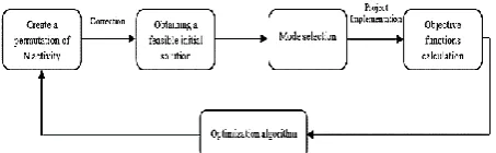
4. 2. The Problem Solving Approach Having explained how to correct an initial solution, we will describe the problem solving process in the general state. Figure 2 illustrates the general scheme of the problem solving process.
Creating and modifying the initial permutation was described in the previous section. In this study, we use a random selection approach to choose the activities modes. In this way, having created possible permutations of activities, we randomly selected a mode from the set of modes related to each activity and then assigned it to that activity.
By project implementation, it is intended to calculate the objective functions by considering the resource constraints. So far, we have managed to produce an initial solution that enables us to extract the starting times of activities and related modes. This initial solution has three components which show the objective functions' values. Presently, using multi objective simulated annealing algorithm and its operators, we search the neighbourhood space of the initial solution in order to improve it and find a better solution.
4. 3. The Multi-Objective Simulated Annealing Algorithm Simulated annealing was independently put forward by Kirkpatrick et al. [29] and Cerny [30]. This method was inspired by what goes on in the process of melting and solidification of metals at the
molecular dimension. To solve combinatorial
optimization problems using simulated annealing algorithm, at each iteration the SA heuristic considers some neighbouring state s' of the current state s and probabilistically decides between moving the system to
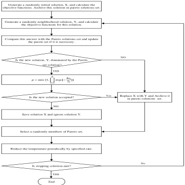
state s' or staying in state s. These probabilities ultimately lead the system to move to states of lower energy. Typically, this step is repeated until the system reaches a state that is good enough for the application. The concept of storing and archiving the Pareto-optimal solutions for solving multi-objective problems with SA has been used by Suppapitnarm et al. [31]. The method enables the search to restart from an archived solution in a solution region, where each of the pair of non-dominated solutions is superior with respect to at least one objective. The flowchart of developed multi-objective simulated annealing algorithm is shown in Figure 3.
5. COMPUTATIONAL RESULTS
In this section, the discussion mentioned in the previous section has been implemented on some instances, and then computational results are reported.
Generate a randomly initial solution, X, and calculate the objective functions. Archive this solution in pareto solutions set .
Generate a randomly neighborhood solution, Y, and calculate the objective functions for this solution.
Compare this ans wer with the Pareto solutions s et and update the pareto set if it is necess ary.
Save solution X and ignore s olution Y. Is the new solution, Y, dom inated by the Pareto
set solution? YES
Is the new solution accepted? NO
Select a randomly members of Pareto set.
Reduce the temperature periodically by specified rate.
Is stopping criterion met?
End YES
Replace X with Y and Archive it in pareto s olutions set. NO
Yes
No
Furthermore, examples of this section are divided into two categories. The first includes four instances known as benchmark instances that evaluate the performance of Multi-objective simulated annealing algorithm. The second category consists of large-scale instances, all of which have been taken from the PSPLIB website. Since some aspects of the study were novel and unique, we had to produce some of the data randomly. For example, financial flows (including receipts and payments) have been produced in each of these instances. All of these examples have been implemented in MATLAB 2012b software and the output was obtained from a PC with a Core i5 2.67 GHz processor.
5. 1. Validation of the Algorithm As it was mentioned in the previous sections, MRCPSPDCF problems are strongly NP-hard, and finding exact solutions for large-scale problems is practically impossible. Considering the fact that real-world problems are usually large-size problems and finding an exact solution for them is either impossible or requires a lot of time, using meta-heuristic methods is inevitable in these cases. Therefore, in this research, a multi-objective Simulated Annealing meta-heuristic algorithm (MOSA) has been developed in order to find credible solutions at a reasonable time.
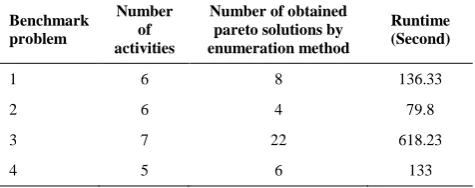
In order to validate the provided algorithm, we consider a set of instances as benchmark examples. This set of benchmark instances includes four different examples whose networks are shown in Figures 4 to 7. The optimal solutions have been obtained by complete enumeration of the solution space. Moreover, the number of optimal solutions and also their execution time for each benchmark instance is mentioned in Table 1. At this moment, we want to solve the benchmark instances using MOSA algorithms so that it can be evaluated in its ability to find optimal solutions.
I
II
III
IV
V
VI 1
2
4 3
5
6
Figure 4. Network of the 1th benchmark instance
I
II
III
IV
V 1
2
3
4
5
6
Figure 5. Network of the 2th benchmark instance
I
II
III
IV
V
VI 1
2
4 3
5
6
7
Figure 6. Network of the 3th benchmark instance
I
II
IV
V 1
3 4
5 2
Figure 7. Network of the 4th benchmark instance
TABLE 1. Results of solving the benchmark instances by the enumeration method
Benchmark problem
Number of activities
Number of obtained pareto solutions by enumeration method
Runtime (Second)
1 6 8 136.33
2 6 4 79.8
3 7 22 618.23
4 5 6 133
As Table 2 indicates, the algorithm has managed to obtain all of the optimal solutions in a short time. Since the algorithm has a good performance in solving small-scale instances, we expect to reach optimal or at least near-optimal solutions in large-scale instances by increasing the number of iterations of algorithm.
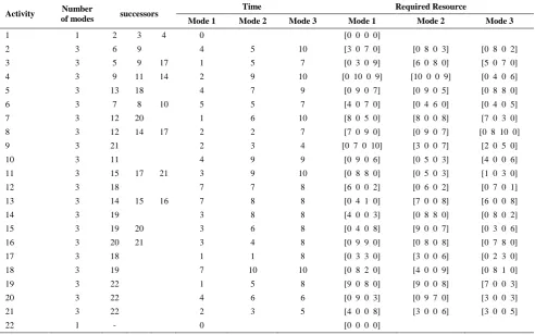
5. 2. Algorithm Performance in Large-Scale Projects The following is two relatively large-scale instances extracted from the PSPLIB website, as mentioned earlier. The first is an example of 20 three-mode activities, and the second is 30 three-three-mode activities. Other information related to the examples is shown in Tables 3 and 4, respectively. Also, the solving results of the first example for 10000 iteration and 10 runs is presented in Table 5.
TABLE 2. Results of solving the benchmark instances by MOSA algorithm
Benchmark problem
Run Number
Number of total pareto solutions
(obtained by enumeration)
Number of obtained pareto
solutions by MOSA algorithm
Number of newly discovered
solutions
Runtime (Second)
Number of required runs to
explore all pareto solutions
runtimes to explore all pareto solutions
(Second)
1
1
8
8 8 0.3
1 0.31
2 8 0 0.3
3 8 0 0.31
4 7 0 0.31
5 7 0 0.31
2
1
4
4 10 0.31
1 0.31
2 4 0 0.31
3 4 0 0.31
4 4 0 0.31
5 4 0 0.31
3
1
22
20 20 3.53
2 7.14
2 20 2 3.61
3 19 0 3.62
4 18 0 3.23
5 20 0 2.97
4
1
6
6 6 0.17
1 0.17
2 6 0 0.17
3 5 0 0.17
4 5 0 0.17
5 5 0 0.17
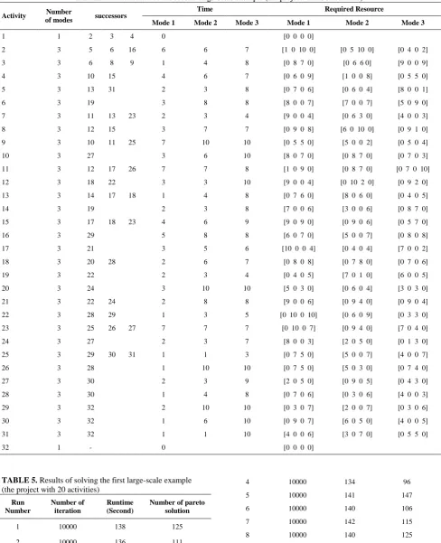
TABLE 3. Data related to the first large-scale example (the project with 20 activities)
Activity Number
of modes successors
Time Required Resource
Mode 1 Mode 2 Mode 3 Mode 1 Mode 2 Mode 3
1 1 2 3 4 0 [0 0 0 0]
2 3 6 9 4 5 10 [3 0 7 0] [0 8 0 3] [0 8 0 2] 3 3 5 9 17 1 5 7 [0 3 0 9] [6 0 8 0] [5 0 7 0] 4 3 9 11 14 2 9 10 [0 10 0 9] [10 0 0 9] [0 4 0 6] 5 3 13 18 4 7 9 [0 9 0 7] [0 9 0 5] [0 8 8 0] 6 3 7 8 10 5 5 7 [4 0 7 0] [0 4 6 0] [0 4 0 5] 7 3 12 20 1 6 10 [8 0 5 0] [8 0 0 8] [7 0 3 0] 8 3 12 14 17 2 2 7 [7 0 9 0] [0 9 0 7] [0 8 10 0] 9 3 21 2 3 4 [0 7 0 10] [3 0 0 7] [2 0 5 0] 10 3 11 4 9 9 [0 9 0 6] [0 5 0 3] [4 0 0 6] 11 3 15 17 21 3 9 10 [0 8 8 0] [0 5 0 3] [1 0 3 0] 12 3 18 7 7 8 [6 0 0 2] [0 6 0 2] [0 7 0 1] 13 3 14 15 16 7 8 8 [0 4 1 0] [7 0 0 8] [6 0 0 8] 14 3 19 3 8 8 [4 0 0 3] [0 8 8 0] [0 8 0 2] 15 3 19 20 3 6 8 [0 4 0 8] [9 0 0 7] [0 3 0 6] 16 3 20 21 3 4 8 [0 9 9 0] [0 8 0 8] [0 7 8 0] 17 3 18 1 1 8 [0 3 3 0] [3 0 0 6] [0 2 3 0] 18 3 19 7 10 10 [0 8 2 0] [4 0 0 9] [0 8 1 0] 19 3 22 1 5 8 [9 0 8 0] [9 0 0 8] [7 0 0 3] 20 3 22 4 6 6 [0 9 0 3] [0 9 7 0] [3 0 0 3] 21 3 22 2 3 5 [4 0 0 8] [3 0 0 6] [3 0 0 5]
TABLE 4. Data related to the second large-scale example (the project with 30 activities)
Activity Number
of modes successors
Time Required Resource
Mode 1 Mode 2 Mode 3 Mode 1 Mode 2 Mode 3
1 1 2 3 4 0 [0 0 0 0]
2 3 5 6 16 6 6 7 [1 0 10 0] [0 5 10 0] [0 4 0 2] 3 3 6 8 9 1 4 8 [0 8 7 0] [0 6 6 0] [9 0 0 9] 4 3 10 15 4 6 7 [0 6 0 9] [1 0 0 8] [0 5 5 0] 5 3 13 31 2 3 8 [0 7 0 6] [0 6 0 4] [8 0 0 1] 6 3 19 3 8 8 [8 0 0 7] [7 0 0 7] [5 0 9 0] 7 3 11 13 23 2 3 4 [9 0 0 4] [0 6 3 0] [4 0 0 3] 8 3 12 15 3 7 7 [0 9 0 8] [6 0 10 0] [0 9 1 0] 9 3 10 11 25 7 10 10 [0 5 5 0] [5 0 0 2] [0 5 0 4] 10 3 27 3 6 10 [8 0 7 0] [0 8 7 0] [0 7 0 3] 11 3 12 17 26 7 7 8 [1 0 9 0] [0 8 7 0] [0 7 0 10] 12 3 18 22 3 3 10 [9 0 0 4] [0 10 2 0] [0 9 2 0] 13 3 14 17 18 1 4 8 [0 7 6 0] [8 0 6 0] [0 4 0 5] 14 3 19 2 3 8 [7 0 0 6] [3 0 0 6] [0 8 7 0] 15 3 17 18 23 4 6 9 [9 0 9 0] [0 9 0 6] [0 5 7 0] 16 3 29 5 8 8 [6 0 7 0] [5 0 0 7] [0 8 0 8] 17 3 21 3 5 6 [10 0 0 4] [0 4 0 4] [7 0 0 2] 18 3 20 28 2 6 7 [0 8 0 8] [0 7 8 0] [0 7 0 6] 19 3 22 2 3 4 [0 4 0 5] [7 0 1 0] [6 0 0 5] 20 3 24 3 10 10 [5 0 3 0] [0 6 0 4] [3 0 3 0] 21 3 22 24 2 8 8 [9 0 0 6] [0 9 4 0] [0 9 0 4] 22 3 28 29 1 3 5 [0 10 0 10] [0 6 0 9] [0 3 3 0] 23 3 25 26 27 7 7 7 [0 10 0 7] [0 9 4 0] [7 0 4 0] 24 3 27 2 3 7 [8 0 0 3] [2 0 5 0] [0 1 3 0] 25 3 29 30 31 1 1 3 [0 7 5 0] [5 0 0 7] [4 0 0 7] 26 3 28 1 10 10 [0 7 5 0] [5 0 3 0] [0 7 4 0] 27 3 30 2 3 9 [2 0 5 0] [0 9 0 5] [0 4 3 0] 28 3 30 1 4 8 [0 7 0 6] [0 3 0 6] [4 0 0 3] 29 3 32 2 10 10 [0 3 0 7] [2 0 0 7] [0 3 0 6] 30 3 32 1 6 10 [0 9 0 7] [6 0 5 0] [4 0 0 5] 31 3 32 1 1 10 [4 0 0 6] [3 0 7 0] [0 5 5 0]
32 1 - 0 [0 0 0 0]
TABLE 5. Results of solving the first large-scale example (the project with 20 activities)
Run Number
Number of iteration
Runtime (Second)
Number of pareto solution
1 10000 138 125 2 10000 136 111 3 10000 150 125
Figure 8. The process of finding the pareto solutions in the project with 20 activities
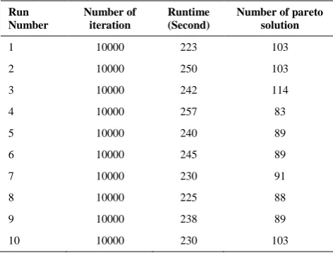
The solving results of the second example for 10000 iterations and 10 runs is presented in Table 6. The process of finding the number of pareto solutions in different iterations can be seen in Figure 9. As can be seen, the process of discovering new pareto solutions is reducing gradually. The fluctuations described in Figure 8 holds true here. The reason might be that a new discovered solution dominates some of the solutions in pareto set, and, as a result, the number of pareto solutions are removed, and the chart has a decreasing trend in some points.
The reason for fluctuations in the chart presented in Figure 8 (that in some parts of the chart the number of pareto solutions is decreased) is that the pareto set is updated continuously, and when a new solution is added to the pareto set, it is compared with all other pareto solutions.
TABLE 6. Results of solving the second large-scale example (the project with 30 activities)
Run Number
Number of iteration
Runtime (Second)
Number of pareto solution
1 10000 223 103
2 10000 250 103
3 10000 242 114
4 10000 257 83
5 10000 240 89
6 10000 245 89
7 10000 230 91
8 10000 225 88
9 10000 238 89
10 10000 230 103
Figure 9. The process of finding the pareto solutions in the project with 30 activities
Obviously, in this comparison it is likely that a new solution dominates some of these solutions. Say answer A dominates answer B, if answer A in any objectives is not worse than answer B, and also the answer A is at least in one of the objectives that is better than answer B. Moreover, if there is not such a situation between A and B, say answer A and B are non-dominated or pareto solutions. That is the reason these dominated solutions have been removed and the number of pareto solutions in these states is lower compared to the previous state (the points that have a decreasing trend in Figure 8).
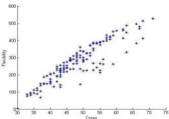
In what follows, we will try to represent the relationship between the objectives functions using the pareto solution points in the solution space for the first example (the project with 20 activities). Additionally, in Figures 11 to 13, mutual influence for objective functions have been presented in the form of two-dimensional graphs.
Figure 11. Mutual influence of NPV-Cmax objective functions
Figure 12. Mutual influence of flexibility-Cmax objective functions
Figure 13. Mutual influence of flexibility-NPV objective functions
Figure 14. The pareto solutions of the project with 20 activities
6. CONCLUSION
Resources constraint project scheduling problem is a practical topic in project management. In this study, in addition to the time-cost trade-off, available incomes in project and flexibility of project against unforeseen events in the form of three objective problems were considered, and their results have been analysed. Since the subject of the research was strongly NP-hard and multi-objective, we developed the multi-objective simulated annealing meta-heuristic algorithm after modelling the problem as a three-objective model to solve the intended model. Also, to validate the algorithm, we applied a complete enumeration to four benchmark instances. The results showed that the algorithm has managed to discover all pareto solutions in a short time. In applying the algorithm in large-scale problems, we attained the results that represent the desirable performance of the algorithm.
As a development for future studies, the presented model in this research can be implemented in a real case study. On the other hand, each of the factors of time and resources may be associated with uncertainty. In this case, the use of fuzzy logic, as a powerful tool, in the study of uncertainty can be considered. In some cases, the decision-maker faces so many pareto solutions that he may get confused in choosing the desired solution. Consequently, considering one of the multi-criteria decision making methods can help the decision maker to do the best choice.
7. REFERENCES
1. Węglarz, J., Józefowska, J., Mika, M. and Waligóra, G., "Project scheduling with finite or infinite number of activity processing modes–a survey", European Journal of Operational Research, Vol. 208, No. 3, (2011), 177-205.
2. Pritsker, A.A.B., Waiters ,L.J. and Wolfe, P.M., "Multiproject scheduling with limited resources: A zero-one programming approach", Management Science, Vol. 16, No. 1, (1969), 93-108.
3. Talbot, F.B., "Resource-constrained project scheduling with time-resource tradeoffs: The nonpreemptive case", Management Science, Vol. 28, No. 10, (1982), 1197-1210.
4. Patterson, J., Słowiński, R., Talbot, F. and Węglarz, J., An algorithm for a general class of precedence and resource constrained scheduling problems, in Advances in project scheduling. 1989, Elsevier.3-28.
5. Zhu, G., Bard, J.F. and Yu, G., "A branch-and-cut procedure for the multimode resource-constrained project-scheduling problem", INFORMS Journal on Computing, Vol. 18, No. 3, (2006), 377-390.
6. Hartmann, S. and Drexl, A., " Project scheduling with multiple modes: A comparison of exact algorithms", Networks: An International Journal, Vol. 32, No. 4, (1998), 283-297. 7. Hartmann, S., "Project scheduling with multiple modes: A
8. Tseng, L.-Y. and Chen, S.-C., "Two-phase genetic local search algorithm for the multimode resource-constrained project scheduling problem", IEEE Transactions on Evolutionary Computation, Vol. 13, No. 4, (2009), .857-848
9. Fahmy, A., Hassan, T.M. and Bassioni, H., "Improving rcpsp solutions quality with stacking justification–application with particle swarm optimization", Expert Systems with Applications, Vol. 41, No. 13, (2014), 5870-5881.
10. Xiao, J., Wu, Z. ,Hong, X.-X., Tang, J.-C. and Tang, Y., "Integration of electromagnetism with multi-objective evolutionary algorithms for rcpsp", European Journal of Operational Research, Vol. 251, No. 1, (2016), 22-35. 11. Zoraghia, N., Najafib, A. and Niaki, S., "Resource constrained
project scheduling with material ordering: Two hybridized meta-heuristic approaches", International Journal of Engineering Transactions C: Aspects, Vol. 28, No. 6 (2015), 896-902.. 12. Ning, M., He, Z., Jia, T. and Wang, N., "Metaheuristics for
multi-mode cash flow balanced project scheduling with stochastic duration of activities", Automation in Construction, Vol. 81, (2017), 224-233.
13. Russell, A., "Cash flows in networks", Management Science, Vol. 16, No. 5, (1970), 357-373.
14. Sung, C. and Lim, S., "A project activity scheduling problem with net present value measure", International Journal of Production Economics, Vol. 37, No. 2-3, (1994), 177-187. 15. Mika, M., Waligóra, G. and Węglarz, J., "Simulated annealing
and tabu search for multi-mode resource-constrained project scheduling with positive discounted cash flows and different payment models", European Journal of Operational Research, Vol. 164, No. 3, (2005), 639-668.
16. Najafi, A.A. and Niaki, S.T.A., "Resource investment problem with discounted cash flows", International Journal of Engineering, Vol. 18, No. 1 (2005), 53-64.
17. Seyfi, M. and Tavakoli, M.R., "A new bi-objective model for a multi-mode resource-constrained project scheduling problem with discounted cash flows and four payment models",
International Journal of Engineering Transactions A: Basics, Vol. 21, No. 4 (2008), 347-360.
18. Leyman, P. and Vanhoucke, M., "Payment models and net present value optimization for resource-constrained project scheduling", Computers & Industrial Engineering, Vol. 91, (2016), 139-153.
19. Huang, X. and Zhao, T., "Project selection and scheduling with uncertain net income and investment cost", Applied Mathematics and Computation, Vol. 247, (2014), 61-71.
20. Kelley Jr, J.E., "Critical-path planning and scheduling: Mathematical basis", Operations research, Vol. 9, No. 3, (1961), 296-320.
21. Moder, J.J. and Phillips, C.R., " Project management with CPM, PERT and precedence diagramming”, (1983).
22. Hindelang, T.J. and Muth, J.F., "A dynamic programming algorithm for decision cpm networks", Operations research, Vol. 27, No. 2, (1979), 225-241.
23. De, P., Dunne, E.J., Ghosh, J.B. and Wells, C.E., "Complexity of the discrete time-cost tradeoff problem for project networks",
Operations Research, Vol. 45, No. 2, (1997), 302-306. 24. Erenguc, S.S., Tufekci, S. and Zappe, C.J., "Solving time/cost
trade‐off problems with discounted cash flows using generalized benders decomposition", Naval Research Logistics (NRL), Vol. 40, No. 1, (1993), 25-50.
25. Icmeli, O. and Erenguc, S.S., "The resource constrained time/cost tradeoff project scheduling problem with discounted cash flows", Journal of Operations Management, Vol. 14, No. 3, (1996), 255-275.
26. Amiria, M.T., Haghighi, F., Eshtehardianc, E. and Abessib, O., "Optimization of time, cost and quality in critical chain method using simulated annealing", International Journal of Engineering Transactions B: Applications , Vol. 30, No. 5 (2017), 627-635.
27. Al-Fawzan, M.A .and Haouari, M., "A bi-objective model for robust resource-constrained project scheduling", International Journal of Production Economics, Vol. 96, No. 2, (2005), 175-187.
28. Ke, H., Wang, L. and Huang, H., "An uncertain model for rcpsp with solution robustness focusing on logistics project schedule",
International Journal of e-Navigation and Maritime Economy, Vol. 3, (2015), 71-83.
29. Kirkpatrick, S., Gelatt, C.D. and Vecchi, M.P., "Optimization by simulated annealing", Science, Vol. 220, No. ,)1983(,4598
671 -680 .
30. Černý, V., "Thermodynamical approach to the traveling salesman problem: An efficient simulation algorithm", Journal of Optimization Theory and Applications, Vol. 45, No. 1, (1985), 41-51.
Project Scheduling with Simultaneous Optimization, Time, Net Present Value, and
Project Flexibility for Multimode Activities with Constrained Renewable Resources
H. Farughi, A. Amiri, F. Abdi
Faculty of Engineering, University of Kurdistan, Sanandaj, Iran
P A P E R I N F O
Paper history:
Received 20 August 2017
Received in revised form 28 January 2018 Accepted 09 March 2018
Keywords:
Resource Constrained Project Scheduling Time-cost trade-off
Simulated Annealing Algorithm Project Flexibility
Multi-mode Activities
هديكچ
یم هدیجنس یفلتخم یاهرایعم ساسا رب هژورپ تیقفوم زا هژورپ ناعفنیذ رظن زا اهرایعم نیا زا مادکره هک دوش
ا توافتم تیمه ی
هژورپ ره تیقفوم یاهرایعم و فادها نیرتمهم زا هنیزه و نامز .تسا رادروخرب یر شهاک رگید فرط زا .دنتسه یا
کس هب طوبرم
تیلاعف مامتا مدع نامز ات ییارجا یاه
شیپ لباقریغ لماوع لیلد هب هدش نییعت شیپ زا یاه رد .دریگ رارق هجوت دروم یتسیاب ینیب
همانرب هلأسم کی بلاق رد هلأسم ندرک هلومرف زا سپ ،رضاح قیقحت مز ندرک هنیمک رد یعس هفده دنچ یزیر
امتا نا ب ،هژورپ م هنیشی
ف شزرا ندرک فاطعنا و هژورپ صلاخ یلع
تیدودحم نتفرگ رظن رد اب هژورپ یریذپ شیپ طباور و عبانم یاه
ین اوخ ،یزا .تشاد میه
هژورپ یریذپ فاطعنا اب
رد رظن نتفرگ کی نامز یروانش یارب اهتیلاعف و هنیشیب ندرک عومجم نیا یاهنامز ،یروانش رظنرد هتفرگ
ف ره ماجنا یارب ،نیا رب هولاع .تسا هدش تلاح هژورپ کی رد تیلاع
گ رظن رد عبانم فرصم زا یفلتخم یاه دش هتفر
هک ،تسا ه
یم باارف متیروگلا زا هلأسم یگدیچیپ هب هجوت اب .ددرگ تیلاعف نآ یارجا هنیزه و نامز رد رییغت ثعاب دناوت هیبش یراکت
س دیربت یزا
بوخ درکلمع هب هجوت اب .تسا هدش هدافتسا لدم لح یارب هفده دنچ نیا هنیهب باوج نتفای رد متیروگلا
م حم لئاس نیا زا ،ک
.تسا هدش هدافتسا گرزب لئاسم رد هنیهب باوج نتفای یارب متیروگلا
doi: 10.5829/ije.2018.31.05b.13