An Application of Fuzzy Logic to Computational Thinking

Vol. 2, No.1, 2012, 18-32

ISSN: 2279-087X (P), 2279-0888(online) Published on 30 November 2012

www.researchmathsci.org

18

Annals of

An Application of Fuzzy Logic to Computational

Thinking

Michael Gr. Voskoglou

School of Technological Applications

Graduate Technological Educational Institute of Patras, Greece E-mail: [email protected], [email protected]

URL: http://eclass.teipat.gr/eclass/corses/523102

Received 28 September 2012; accepted 29 November 2012

Abstract. Computational thinking (CT) is a new problem solving method named for its extensive use of computer science techniques. In this paper we use principles of fuzzy logic to develop a mathematical model representing the CT and the centre of mass of the graph of the membership function involved to obtain a measure of students’ CT skills. We also present two classroom experiments performed recently at the Graduate Technological Educational Institute (TEI) of Patras, Greece illustrating the use of our fuzzy model in practice.

AMS Mathematics Subject Classification (2010): 03E72, 97C80

Keywords: Fuzzy sets and logic, centre of mass of a fuzzy graph, computational and critical thinking, problem solving, mathematical modelling.

1. Introduction

Computational thinking (CT) is a new problem solving method named for its extensive use of computer science techniques. It synthesizes critical thinking and existing knowledge and applies them to solve complex real world technological problems. Actually, the relationship between CT and critical thinking, the two modes of thinking in solving problems, has not been yet clearly established. In a recent paper [13] we have attempted to shed some light into this relationship. According to Liu and Wang [6] CT is a hybrid of the following modes of thinking:

Logical thinking, the process in which one uses reasoning consistency to come to a conclusion. Some computer problems or computer states (situations) involving logical thinking always call for mathematics structure, for relationships between some hypotheses and given statements, and for a sequence of reasoning that makes the conclusion more reasonable.

Modelling thinking, which refers to the translation of objects or phenomena from the real world into mathematical equations (mathematical models) or computer relations (simulation models). It is choosing an appropriate representation for modelling the relevant aspects of a problem to make it tractable.

Constructive thinking, a well-defined computational procedure that takes some value, or set of values as input and produces some value, or set of values as output.

One could claim that modelling thinking constitutes the essence of CT, since it synthesises all the other components of CT (abstract, logical and constructive thinking) for the solution of the corresponding problem. In fact, it is well known (e.g. [8]; paragraph 1.4) that the main stages of the modelling process involve:

• Analysis of the given problem, i.e. understanding of its statement and recognizing limitations, restrictions and requirements of the real system (critical thinking).

• Construction of the model (abstract thinking).

• Solution of the model, achieved by proper logical manipulation (logical thinking).

• Validation (control) of the model, usually achieved by reproducing through it the behaviour of the real system under the conditions existing before the solution of the model (empirical results, special cases etc).

• Implementation of the final results to the real system, i.e.‘translation’ of the solution obtained in terms of the model to the ‘language’ of the real situation in order to reach the required practical conclusions needed for the solution of the given real problem (constructive thinking).

The most important type of model in use is the symbolic or mathematical model. In formulating this type one assumes that all relevant variables are quantifiable. These variables are then related by the appropriate mathematical relations (functions, equations, inequalities, etc) to describe the behaviour of the system and the solution of the model is achieved by proper mathematical manipulation. In this case the stage of the construction of the model is usually called mathematization and presupposes the formulation of the real situation in so that it is ready for mathematical treatment (for more details see [3] and its references).

20 2. The fuzzy model

The stages of the modelling process presented above are helpful in understanding the modellers’ ‘ideal behaviour’, in which they proceed from real world problems through a model to acceptable solutions and report on them. However, things in real situations are usually not happening like that. For example, recent research, ([1], [2], etc), reports that students in school take

individual modelling routes when tackling mathematical modelling problems, associated with their individual learning styles. The human cognition utilizes in general concepts that are inherently graded and therefore fuzzy. On the other hand, from the teacher’s point of view there usually exists vagueness about the degree of students’ success in each of the stages of the modelling process. All these gave us the impulsion to introduce principles of fuzzy sets theory in order to describe in a more effective way the process of modelling in particular and of CT in general. For general facts on fuzzy sets we refer freely to the book [4]. For the development of our fuzzy model we consider a group of n modellers, n

≥

2, working (each one individually) on the same modelling problem. In order to make our model technically simpler, we can, without loss of the generality, reduce the stages of the modelling process to the following three:

• S1 : Analysis/Construction of the model.

• S2 : Solution of the model.

• S3 : Validation of the model/Implementation to the real system.

In fact, the analysis of the given problem is an introductory stage of the modelling process that can be naturally seen as being a sub step of the construction of the model. Further, the stage of implementation of the final results to the real system is an expected action following the validation of the model, which means that the joined stage of Validation/Implementation can be actually considered as the final stage of the modelling process.

Denote by a, b, c, d, and e the linguistic labels of very low, low, intermediate, high and very high success respectively of a system’s entity in each of the Si’s.

Set

U = {a, b, c, d, e}

We are going to attach to each stage Si of the modelling process, i=1,2,3 , a

fuzzy subset, Ai of U. For this, if nia, nib, nic, nid and nie denote the number of

modellers that faced very low, low, intermediate, high and very high success at stage Si respectively, i=1,2,3, we define the membership function mAi for each x

4 4 1,

5 5

3 4

0,75,

5 5

2 3

( ) 0,5,

5 5

2 0, 25,

5 5

0, 0

5

i

ix

ix

A ix

ix

ix

n n

if n

n n

if n

n n

m x if n

n n

if n

n

if n

 _{< ≤}

 

 _{< ≤}

  

= < ≤



 _{< ≤}

 

 _{≤ ≤}



In fact, if one wanted to apply ‘probabilistic’ standards in measuring the degree of success of the modellers at each stage of the process, then he/she should use the relative frequencies nix

n . Nevertheless, such an action would be highly questionable, since the nix‘s are obtained with respect to the linguist labels

of U, which are fuzzy expressions by themselves. Therefore the application of a fuzzy approach by using membership degrees instead of probabilities seems to be more suitable for this case. But, as it is well known, the membership function needed for such purposes is usually defined empirically in terms of logical or/and statistical data. In our case the above definition of

i A

m seems to be

compatible with the common logic.

Then the fuzzy subset Ai of U corresponding to Si has the form:

Ai = {(x, mAi(x)): x∈U}, i=1, 2, 3.

In order to represent all possible profiles (overall states) of the system’s entities during the corresponding process we consider a fuzzy relation, say R, in

U3 _{of the form:}

R= {(s, mR(s)): s=(x, y, z) ∈U3}.

For determining properly the membership function mR we give the following

definition:

A profile s=(x, y, z), with x, y, z in U, is said to be well ordered if x corresponds to a degree of success equal or greater than y and y corresponds to a degree of success equal or greater than z.

For example, (c, c, a) is a well ordered profile, while (b, a, c) is not. We define now the membership degree of a profile s to be

mR(s) = mA₁(x)mA2(y)mA3(z)

if s is well ordered, and 0 otherwise.

In fact, if for example the profile (b, a, c) possessed a nonzero membership degree, how it could be possible for a modeller, who has failed in solving the model, to perform satisfactorily at the validation of it?

22

Ps=

3

s s s U

m m ∈

∑

We define also the possibilityrs of s to be rs=

} max{ s

s

m

m _,

where max{ms} denotes the maximal value of ms, for all s in U3. In other words

the possibility of s expresses the “relative membership degree” of s with respect to max{ms}.

Assume further that one wants to study the combined results of behaviour of k

different groups of a system’s entities, k

≥

2, during the same process. For this, we introduce the fuzzy variables A1(t), A2(t) and A3(t) with t=1, 2,…, k. The

values of these variables represent fuzzy subsets of U corresponding to the stages of the modelling process for each of the k groups; e.g. A1(2) represents the fuzzy

subset of U corresponding to the stage of Analysis/construction of the model for the second group (t=2). It becomes evident that, in order to measure the degree of evidence of the combined results of the k groups, it is necessary to define the probability p(s) and the possibility r(s) of each profile s with respect to the membership degrees of s for all groups. Therefore we introduce the pseudo-frequencies

f(s) =

_∑

=

k t

s t

m

1

) (

and we define the probability and possibility of a profile s by p(s) =

3

( ) ( )

s U

f s f s ∈

∑

and r(s) =

)} ( max{

) (

s f s

f _{respectively, where max{f(s)} denotes the maximal}

pseudo-frequency.

Obviously the same method could be applied when one wants to study the combined results of behaviour of a group during k different modelling situations. The above model gives, through the calculation of probabilities and possibilities of all modellers’ possible profiles, a quantitative view of their realistic performance in all stages of the modelling process.

3. Measuring model building and CT capacities

The amount of information obtained by an action can be measured by the reduction of uncertainty resulting from this action. Accordingly a system’s uncertainty is connected to its capacity in obtaining relevant information. Therefore a measure of uncertainty could be adopted as a measure of a system’s effectiveness in solving related problems. Based on this fact, we have used uncertainty measures in assessing the effectiveness of several systems in Education, Artificial Intelligence and Management [11].

In this paper and in terms of the fuzzy model developed above we shall introduce another approach for measuring model building capacities (and hence CT capacities as well), known as the ‘centroid method’. According to this method the centre of massof the graph

of the membership function involved

provides an alternative measure of the system’s performance.

The application of the ‘centroid method’ in practice is simple and evident and, in contrast to the measures of uncertainty, needs no complicated calculations in its final step.

For this, given a fuzzy subset A = {(x, m(x)): x∈U} of the universal set U of the discourse with membership function m: U

→

[0, 1], we correspond to each

x∈U an interval of values from a prefixed numerical distribution, which actually means that we replace U with a set of real intervals. Then, we construct the graph

F of the membership function y=m(x).There is a commonly used in fuzzy logic approach to measure performance with the pair of numbers (xc, yc) as the

coordinates of the centre of mass, sayFc, of the graph F, which we can calculate

using the following well-known [9] formulas:

,

F F

c c

F F

xdxdy ydxdy

x y

dxdy dxdy

=

∫∫

=

∫∫

∫∫

∫∫

(1)

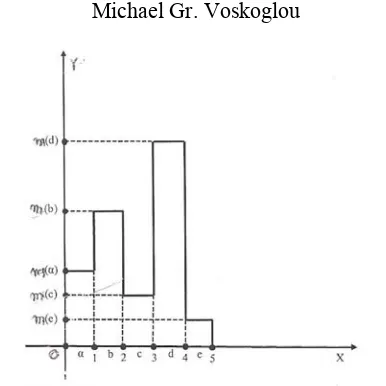
Concerning the modelling process, when a student obtains a mark, say y, we characterize his/her performance as very low (a) if y ∈ [0, 1) , as low (b) if y ∈ [1, 2), as intermediate (c) if y∈ [2, 3), as high (d) if y ∈ [3, 4) and as very high

(e) if y ∈ [4,5] respectively. Therefore in this case the graph F of the

corresponding fuzzy subset of U is the bar graph of Figure 3.

It is easy to check that, if the bar graph consists of n rectangles (in Figure 3 we have n=5), the formulas (1) can be reduced to the following formulas:

2

1 1

1 1

(2 1)

1 1

,

2 2

n n

i i

i i

c n c n

i i

i i

i y y

x y

y y

= =

= =

 ₋   

   

   

= =

   

   

   

∑

∑

∑

∑

24

Figure 3: Bar graphical data representation

Indeed, in this case

F

dxdy

∫∫

is the total mass of the system which is

equal to

1 n i i y =

∑

,

F xdxdy

∫∫

is the moment about the y-axis which is equal

to

1 1 0 1

i

i

y i

n n

i F i i

xdxdy dy xdx

= = − =

∑

∫∫

∑

∫ ∫

1 1 i n i i i y xdx = − =

∑ ∫

= 1

1 _{(2 1)} 2 n i i i y = −

∑

, and

F

ydxdy

∫∫

is the

moment about the y-axis which is equal to

1 1 0 1

i

i

y i

n n

i F i i

ydxdy ydy dx

= = −

=

∑

∫∫

∑

∫

∫

=

1 1 0 1

i

i

y i

n n

i F i i

xdxdy dy xdx

= = −

=

∑

∫∫

∑

∫ ∫

=

2

10 1

1 2 i y n n i i i ydy y = = =

∑

∫

∑

.

From the above argument, where Fi, i=1,2,…,n , denote the n rectangles of

the bar graph, it becomes evident that the transition from (1) to (2) is obtained under the assumption that all the intervals have length equal to 1 and that the first of them is the interval [0, 1].

In our case (n=5) formulas (2) are transformed into the following form:

(3)

1 2 3 4 5

1 2 3 4 5

2 2 2 2 2

1 2 3 4 5

1 2 3 4 5

3 5 7 9

1 , 2 1 _. 2 c c

y y y y y

x

y y y y y

y y y y y

y

y y y y y

Normalizing our fuzzy data by dividing each m(x), x∈U, with the sum of all membership degrees we can assume without loss of the generality that

y1+y2+y3+y4+y5 = 1. Therefore we can write:

(

)

(

)

1 2 3 4 5

2 2 2 2 2

1 2 3 4 5

1

3 5 7 9 ,

2 1 2

c

c

x y y y y y

y y y y y y

= + + + +

= + + + +

(4)

with yi =

∑

∈U x

i

x m

x m

) (

) (

, where x₁= a, x2 =b, x3= c, x4 = d and x5 = e.

But 0

≤

(y1-y2)2=y12+y22-2y1y2 , therefore y12+y22

≥

2y1y2 ,with the equality

holding if, and only if, y1=y2.

In the same way one finds that y12+y32

≥

2y1y3, and so on. Hence it is easy to

check that (y1+y2+y3+y4+y5)2

≤

5(y12+y22+y32+y42+y52), with the equality

holding if, and only if y1=y2=y3=y4=y5.

But y1+y2+y3+y4+y5 =1, therefore 1

≤

5(y12+y22+y32+y42+y52) (5),with the

equality holding if, and only if y1=y2=y3=y4=y5= 5 1 _.

Then the first of formulas (4) gives that xc =

2

5_{. Further, combining the}

inequality (5) with the second of formulas (4) one finds that 1

≤

10yc, or yc

≥

10 1

Therefore the unique minimum for yc corresponds to the centre of mass Fm (

2 5_,

10 1 _).

The ideal case is when y1=y2=y3=y4=0 and y5=1. Then from formulas (3) we

get that xc =

2 9 _{and y}

c =

2

1_{.Therefore the centre of mass in this case is the point}

Fi (

2 9_,

2 1_).

On the other hand the worst case is when y1=1 and y2=y3=y4= y5=0. Then for

formulas (3) we find that the centre of mass is the point Fw (

2 1_,

2

1_{). Therefore the}

“area” where the centre of mass Fc lies is represented by the triangle Fw Fm Fi of

Figure 4.Then from elementary geometric considerations it follows that for two groups of a system’s objects with the same xc

≥

2,5 the group having the centre

of mass which is situated closer to Fi is the group with the higher yc; and for two

groups with the same xc <2.5 the group having the centre of mass which is

situated farther to Fw is the group with the lower yc. Based on the above

26

Figure 4. Graphical representation of the “area” of the centre of mass

• Among two or more groups the group with the biggest xc performs better.

• If two or more groups have the same xc ≥ 2.5, then the group with the higher yc performs better.

• If two or more groups have the same xc < 2.5, then the group with the lower yc performs better.

Notice that Subbotin et al., based on our fuzzy model for the process of learning [10], have applied the “centroid” method on comparing students’ mathematical learning abilities [7]. More recently we have applied together with I. Subbotin the above method in assessing students’ Analogical Reasoning skills [12].

5. Classroom Experiments

The role that the rational use of the new technologies could play for the development of students’ PS abilities is very important indeed. In fact, the animation of figures and mathematical representations, provided by suitable computer software packages, videos, etc, increases the students’ imagination and helps them in finding solutions easier of the corresponding problems. The role of mathematical theory after this is not to convince, but to explain.

Exploratory investigations have demonstrated how exposure to CT enhances the way students approach problems ([5], [13], [14], etc). In our will to explore further the effect of the use of computers as a tool in solving mathematical problems we performed during the academic year 2011-12 the following classroom experiments:

“Higher Mathematics I” 1 of their first term of studies. The students, who had no programming experience, where divided in two groups of 35 and 30 students respectively. In the second (control) group the lectures were performed in the classical way on the board, followed by a number of exercises and examples connecting mathematics with real world applications and problems. The students participated in solving these problems.

The difference for the first (experimental) group was that part (about the1

3) of

the lectures and the exercises were performed in a computer laboratory. There the instructor used the suitable technological tools (computers, video projections, etc) to present the corresponding mathematical topics in a more “live” and attractive manner to students’, while the students themselves, divided in small groups, used the existing ready mathematical software to solve the problems with the help of computers. Notice that all students (of both groups) were learning in a parallel course (Computer Science I) among the other basics about computers and the use of one of the well known mathematical software packages.

At the end of the term all students passed the final written examination of the mathematics course for the assessment of their progress. The examination involved a number of general theoretical questions and exercises covering all the topics taught and three simplified real world problems (see Appendix) requiring mathematical modeling techniques for their solution (time allowed was three hours). We marked the students’ papers separately for the questions and exercises and separately for the problems.

In assessing the general performance of the two groups we applied the GPA method2 _{commonly used in the USA and other countries. According to the marks}

obtained no significant differences were found for the two groups concerning the part of theoretical questions and exercises. On the contrary, the performance of the experimental group was found to be significantly better in solving the problems (GPA1 ≈ 2.49, GPA2 = 2).

In our will to analyze deeper the results of the above experiment we applied our fuzzy model developed in the previous two sections. In fact, examining students’ papers of the experimental group we found that 15, 12 and 8 students

had intermediate, high and very high success respectively at stage S1 of

analysis/mathematization. Therefore we have n1a=n1b=0, n1c=15, n1d=12 and

1 _{The course involves Differential and Integral Calculus in one variable, Elementary}

Differential Equations and Linear Algebra.

2 _{Te Great Point Average (GPA) is a weighted average of the students’ performance. For} this, each student’s paper is marked with A (90-100%), B (80-90%), C(80-70%), D (60-70%), or F (< 60%). Then, if n is the total number of students and n_A,n_B,n_C,n_D,n_F denote the numbers of students getting the marks A, B, C, D, F respectively, GPA =

n n n n

n 1. 2. 3 4. .

28

n1e=8. Thus, by the definition of the corresponding membership function given in

section 3, S1 is represented by a fuzzy subset of U of the form:

A1 = {(a,0),(b,0),(c, 0.5),(d, 0.25),(e,0..25).

In the same way we represented the stages S2 and S3 as fuzzy sets in U by

A2= {(a,0),(b,0),(c, 0.5),(d, 0.25),(e,0)} and

A3 = {(a, 0.25),(b, 0.25),(c, 0.25),(d,0),(e,0)} respectively.

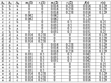
Next we calculated the membership degrees of the 53 _{(ordered samples}

with replacement of 3 objects taken from 5) in total possible students’ profiles as it is described in section 3 (see column of ms(1) in Table 1). For example, for the

profile s=(c, c, a) one finds that

ms = mA₁(c). mA2(c). mA3(a) = 0.5 x 0 .5 x 0.25 = 0.06225.

Further, from the values of the column of ms(1) it turns out that the

maximal membership degree of students’ profiles is 0.06225. Therefore the possibility of each s in U3_{is given by}

rs=

0.06225

s

m

.

Working as above we found for the control group that

A1={(a, 0),(b, 0.25),(c, 0.5),(d, 0.25),(e, 0)},

A2={(a, 0.25),(b, 0.25),(c, 0.5),(d, 0),(e, 0)}

A3={(a, 0.25),(b, 0.25),(c, 0.25),(d, 0),(e, 0)}

and we calculated the membership degrees ms(2) and the possibilities rs(2) of its

students (see the corresponding columns in Table 1).

Next, in order to obtain a quantitative view of the combined results of the two groups’ performance, we calculated the pseudo-frequencies f(s) of all modellers’ profiles and the corresponding possibilities r(s) (see the last two columns of Table 1)

Finally, on comparing the two groups performance let us denote by Aij the

fuzzy subset of U attached to the stage Sj , j=1,2,3 , of the modelling process

with respect to the student group i, i=1,2.

At the first stage of analysis/mathematization we have A11 = {(a, 0),(b, 0),(c, 0.5),(d, 0.25),(e, 0.25)

A21= {(a, 0),(b, 0.25),(c, 0.5),(d , 0.25),(e, 0)}

and respectively

xc11 =

2

xc21 =

2

1_{(3 x 0.25 + 5 x 0.5 + 7 x 0.25) = 2.25}

By our criterion obtained in section 4 the first (experimental) group demonstrates better performance.

Table 1: Profiles with non zero membership degrees

A1 A2 A3 ms(1) rs(1) ms(2) rs(2) f(s) r(s)

b b b 0 0 0.016 0.258 0.016 0.129

b b a 0 0 0.016 0.258 0.016 0.129

b a a 0 0 0.016 0.258 0.016 0.129

c c c 0.062 1 0.062 1 0.124 1

c c a 0.062 1 0.062 1 0.124 1

c c b 0 0 0.031 0.5 0.031 0.25

c a a 0 0 0.031 0.5 0.031 0.25

c b a 0 0 0.031 0.5 0.031 0.25

c b b 0 0 0.031 0.5 0.031 0.25

d d a 0.016 0.258 0 0 0.016 0.129

d d b 0.016 0.258 0 0 0.016 0.129

d d c 0.016 0.258 0 0 0.016 0.129

d a a 0 0 0.016 0.258 0.016 0.129

d b a 0 0 0.016 0.258 0.016 0.129

d b b 0 0 0.016 0.258 0.016 0.129

d c a 0.031 0.5 0.031 0.5 0.062 0.5

d c b 0.031 0.5 0.031 0.5 0.062 0.5

d c c 0.031 0.5 0.031 0.5 0.062 0.5

e c a 0.031 0.5 0 0 0.031 0.25

e c b 0.031 0.5 0 0 0.031 0.25

e c c 0.031 0.5 0 0 0.031 0.25

e d a 0.016 0.258 0 0 0.016 0.129

e d b 0.016 0.258 0 0 0.016 0.129

e d c 0.016 0.258 0 0 0.016 0.129

(The outcomes of the above Table were obtained with accuracy up to the third decimal point)

At the second stage of solution we have:

A12 = {(a, 0),(b, 0),(c, 0.5),(d, 0.25),(e, 0)},

A22={(a, 0.25),(b, 0.25),(c, 0.5),(d, 0),(e, 0)}.

Normalizing the membership degrees in the first of the above fuzzy subsets of U (0.5 : 0,.75 ≈ 0.67 and 0.25 : 0.75 ≈ 0.33) we get

A12 = {(a, 0),(b, 0),(c, 0.67),(d, 0.33),(e, 0)},

A22={(a, 0.25),(b, 0.25),(c, 0.5),(d, 0),(e, 0)}

and respectively

x

c12

=

2

1_{(5 x 0.67 + 7 x 0.33) = 2.83}

30

By our criterion, the first group again demonstrates a significantly better performance.

Finally, at the third stage of validation/implementation we have

A13= A23 = {(a, 0.25),(b, 0.25),(c, 0.25),(d, 0),(e, 0)},

which obviously means that at this stage the performances of both groups are identical.

Based on our calculations we can conclude that the experimental group demonstrated a significantly better performance at the stages of analysis/mathematization and of solution, but performed identically with the control group at the stage of validation/implementation.

At the same chronological period the same experiment was performed under similar conditions with two groups of students of the School of Management and Economics of the TEI of Patras (50 students in each group). In this case the performance of the control group was found to be slightly better for the first part of the examination (questions and exercises), but the performance of the experimental group was found again to be better for the second part (problems). In concluding, the results of our experiments give a strong indication that the use of computers as a tool for PS enhances the students’ abilities in solving real world mathematical problems by using CT.

5. Discussion and Conclusions

The following conclusions can be drawn from the discussion performed in this paper:

• Modelling thinking constitutes the essence of CT, since it synthesises all the other components of CT (abstract, logical and constructive thinking) for the solution of the corresponding problem.

• In this paper we developed a fuzzy model for the CT process by

representing the main stages of the modelling process as fuzzy subsets of a set of linguistic labels characterizing the modellers’ performance in each of these stages. We also applied the ‘centroid’ method in obtaining a measure of the individuals’ CT skills.

• Two classroom experiments were presented illustrating the use of our

fuzzy model in practice. The results of these experiments give a strong indication that the use of computers as a tool for problem solving enhances the students’ abilities in solving real world problems involving mathematical modelling. This is also crossed by us and by other researchers in earlier papers.

derivatives, integrals, etc, and even more to obtain all the existing alternative proofs of the basic mathematical theorems and in some cases to produce new ones. Based on the above facts a number of scientists, mainly among the specialists of Computer Science, have already reached to the conclusion that teachers will not be needed in future for the development of students’ knowledge base and learning skills, since everything could be done by the computers (possibly at home). “The use of horses is not necessary, from the time that cars were invented”, argue some of them.

But, this is actually an illusion! In fact, the acquisition of information is valuable for the learner, but the most important thing is to learn how to think rationally and creatively. The latter is impossible to be succeeded through the help of computers only, because computers have been created by humans and, although they dramatically exceed in speed and memory, they will never reach, at least according to the standard logic, the quality of human thinking. On the other hand, the practice of students with numerical, algebraic and analytic calculations, with the solution of problems and the rediscovery of proofs of the known mathematical theorems, must be continued for ever; otherwise they will gradually loose the sense of numbers and symbols, the sense of space and time, and they will become unable to create new knowledge and technology.

REFERENCES

1. Borroneo Ferri, R. Modelling problems from a cognitive perspective, in

Haines, C.R., Galbraith, P., Bloom, W., Khan, S. (Eds.), Mathematical

Modelling: Education, Engineering and Economics, (ICTMA 12) (2007) 260-270, Chichester: Horwood Publishing.

2. Doer, H.M., What knowledge do teachers need for teaching Mathematics

through applications and modeling? In Blum, W., Galbraith, P.L., Henn,

H-W.and Niss, M. (Eds.), Modelling and Applications in Mathematics

Education, (2007) 69-78.

3. Haines, C.R. and Crouch, R., Remarks on modeling cycle and interpretation of behaviours, in Lesh, R. A., Galbraith, P. L., Haines, C.R. & Harford, A.

(Eds.), Modelling Students’ Mathematical Modelling Competencies,

(ICTMA13) (2010) 145-154.

4. Klir, G. J. and Folger, T. A., Fuzzy Sets, Uncertainty and Information, London, UK: Prentice Hall, 1988.

5. Lewandowski, G., Bouvier, D. , McCartney, R. , Sanders, K. and Simon, B., Common sense computing (episode 3): Concurrency and concert tickets. In ICER ’07: Proceedings of the Third International Workshop on Computing Education Research, 2007.

6. Liu, J. and Wang, L., Computational Thinking in Discrete Mathematics,

IEEE 2nd _{International Workshop on Education Technology and Computer} Science, (2010) 413-416.

7. Subbotin, I. Ya., Badkoobehi, H. & Bilotskii, N., Application of Fuzzy Logic

to Learning Assessment, Didactics of Mathematics: Problems and

32

8. Taha, H. A., Operations Research-An Introduction, 2nd _{edition, Collier}

Macmillan, N. Y., London, 1967.

9. van Broekhoven, E. & De Baets, B., Fast and accurate center of gravity defuzzification of fuzzy system outputs defined on trapezoidal fuzzy partitions, Fuzzy Sets and Systems, 157(7) (2006) 904-918.

10. Voskoglou, M. Gr., The Process of Learning Mathematics: A Fuzzy Set Approach, Heuristics and Didactics of Exact Sciences, 10, 9-13, 1999.

11. Voskoglou, M. Gr., Stochastic and fuzzy models in Mathematics Education, Artificial Intelligence and Management, Lambert Academic Publishing, Saarbrucken, Germany, 2011 (for more details look at

http://amzn.com./3846528218 ).

12. Voskoglou, M. Gr. & Subbotin, I. Ya., Fuzzy Models for Analogical

Reasoning, International Journal of Applications of Fuzzy Sets, 2, 19-38, 2012.

13. Voskoglou, M. G. & Buckley, S., Problem Solving and Computers in a Learning Environment, Egyptian Computer Science Journal, 36(4) (2012) 28-46.

14.Weller, K. et al., Student performance and attitudes in courses based on APOS theory and theACE teaching style, in A. Selden et al. (Eds.), Research in collegiate mathematics education V, 97-131, Providence, RI: American Mathematical Society, 2003.

Appendix

The problems given for solution to students in our classroom experiments: Problem 1: We want to construct a channel to run water by folding the two edges of an orthogonal metallic leaf having sides of length 20cm and 32 cm, in such a way that they will be perpendicular to the other parts of the leaf. Assuming that the flow of the water is constant, how we can run the maximum possible quantity of the water?

Remark: The correct solution is obtained by folding the edges of the longer side of the leaf. Some students solved the problem by folding the edges of the other side and failed to realize (validation of the model) that their solution was wrong.

Problem 2: Let us correspond to each letter the number showing its order into the alphabet (A=1, B=2, C=3 etc). Let us correspond also to each word consisting of 4 letters a 2X2 matrix in the obvious way; e.g. the matrix













5

13

15

19

corresponds to the word SOME. Using the matrix E=

_











7

11

5

8

as an

encoding matrix how you could send the message LATE in the form of a camouflaged matrix to a receiver knowing the above process and how he (she) could decode your message?