M/M/2/k Loss and Delay Interdependent Queueing Model with Controllable Arrival Rates, No Passing and Feedback

Vol. 15, No. 1, 2017, 13-24

ISSN: 2279-087X (P), 2279-0888(online) Published on 11 December 2017

www.researchmathsci.org

DOI: http://dx.doi.org/10.22457/apam.v15n1a2

13

Annals of

M/M/2/k Loss and Delay Interdependent Queueing Model

with Controllable Arrival Rates, No Passing and Feedback

G. Rani1 and V. Shanthi2

1

PG & Research Department of Mathematics, Seethalakshmi Ramaswami College Tiruchirappalli – 620 002, Tamil Nadu, India.

E-mail: [email protected]

2

Department of Mathematics, Seethalakshmi Ramaswami College Tiruchirappalli – 620 002, Tamil Nadu, India.

E-mail: varadarajanshanthi@ yahoo.com Received 2 November 2017; accepted 5 December 2017

Abstract. In this paper M/M/2/k loss and delay queueing model with controllable arrival rates, 2-server with identical service rates, no passing and feedback is considered. For this model, the steady state solution, the system characteristics are derived and the average waiting time for the two types of customers (Elective and Emergency) either with feedback or without feedback is obtained for varying arrival rates when the arrival and service processes are independent. The analytical results are numerically illustrated and the effect of the nodal parameters on the system characteristics are studied and relevant conclusion is presented.

Keywords: Controllable arrival rates, Finite capacity, Elective and Emergency Customers, No passing, Two server with parallel channels, Feedback.

AMS Mathematics Subject Classification (2010): 60K25, 68M20, 90B22 1. Introduction

Queuing system presents a concrete framework for design and analysis of practical applications. Queueing models provide the predictions of behaviour of systems such as waiting times, the average number of waiting customers and so forth. It is used in academic programs of Industrial Engineering, Computer Engineering etc., as well as in programs of Telecommunication and Computer Science. These predictions help us to anticipate situations to take appropriate measures to shorten the queues. Due to restriction of no passing the customers are allowed to depart from the system in the chronological order of their arrival either with feedback or without feedback. In the loss and delay queueing system the customers are classified into two classes. They are (a) Elective customers and (b) Emergency customers either with feedback or without feedback. The Elective customers have patience to form a queue and wait while the Emergency customers finding the server busy on their arrival, leave the system and are lost. But in many real life situations, the arrival and service patterns are interdependent.

14

M/M/c/k interdependent queueing model with controllable arrival rates and feedback. Srinivasan and Thiagarajan [7] have discussed a finite capacity multiserver Poisson input queue with interdependent inter-arrival service time and controllable arrival rates. Rani and Srinivasan [6] have analysed M/M/c/k loss and delay interdependent queueing model with controllable arrival rates, no passing and feedback. Kalyanaraman and Sumathy [3] have studied a feedback queue with multiple servers and batch service. Thangaraj and Shanthakumaran [8] studied a queue with a Markovian feedback. This paper is organized as follows: In section 2 a mathematical model for a M/M/2/k loss and delay with 2-server in the same service rate interdependent queueing model with controllable arrival rates, no passing and feedback is described. In section 3 postulates of the model are stated. In section 4 the steady state equations of the model are framed. In section 5 the system characteristics are considered and the average waiting times for the two types of customers (Elective and Emergency) either with feedback or without feedback are obtained for varying arrival rates. And finally in the section 6 the analytical results are numerically illustrated, and the effect of the nodal parameters on the system characteristics are studied and relevant conclusion is presented.

The diagrammatic representation of M/M/2/k loss and delay queueing system with Bernoulli feedback

Feedback arrivals +

Regular arrivals Input

Elective customers

Emergency customers

Queue

C1

C2

Parallel Servers

Output Departure 2-Server finite capacity

Feedback arrivals

Figure 1:

• Due to restriction of no passing

• The elective customers have patience to form a queue and wait while the emergency customers finding the server busy on their arrival either with feedback or without feedback, leave the system and are lost.

2. Description of the model

No Passing and Feedback

15

arrivals and feedback arrivals. The Elective and Emergency customers are served according to the first come first served rule with following assumptions.

The arrival process {X1(t)} and the service process {X2(t)} of the system are

correlated and follow a bivariate Poisson process given by

P{X1(t) = x1, X2(t) = x2} =

[

]

1 2

1 2

min( , )

( )

0

1 2

( )

!( )!( )!

ij n

x x

x k x k k

ij n

k

e t

k x k x k

λ µ ε _{ε λ ε} − _{µ ε} −

− + −

=

 ₋  ₋

 

− −

∑

x1, x2 = 0, 1, 2, 3, ..., λij, µn > 0, i = 0, 1 and j = 1, 2

n = 0, 1, 2, ..., c – 1, c, c + 1, ..., r – 1, r, r + 1, ..., R – 1, R, R + 1, ..., k – 1, k with parameters λ01, λ02, λ11, λ12, µn and ε as mean arrival rate of Elective customers,

mean arrival rate of Emergency customers, when the system is in the faster rate of arrivals either with feedback or without feedback, mean arrival rate of Elective customers, mean arrival rate of Emergency customers, when the system is in the slower rate of arrivals either with feedback or without feedback, mean service rate and mean dependence rate (co-variance between arrival and service processes) respectively.

Also the mean arrival rate and mean service rate when the system is of size n is defined as

λij = 0 01 1

; 0 ; 1, 2

; 1

; 1 ; 1, 2

j

j

n c j

c n R

r n k j

λ δ λ δ λ δ

≤ < =

 

≤ ≤ −



 _{+ ≤ ≤ =}



µn =

; 0

;

nq n c

cq c n k

µ µ

≤ <

 

≤ ≤



3. The postulates of the model

1. Probability that there is no arrival (Elective and Emergency) and no service completion during a small interval of time h, when the system is with λij, i = 0, 1 & j = 1, 2 faster (slower) rate of arrivals either with feedback or without feedback, is

1 – [(λij – ε)δ + p(µ – ε)2 + q(µ – ε)2]h + o(h)

2. Probability that there is one arrival (Elective and Emergency) and no service completion during a small interval of time h, when the system is with λij, i = 0, 1 & j = 1, 2 faster (slower) rate of arrivals either with feedback or without feedback, is

(λij – ε)δ + o(h)

3. Probability that there is no arrival (Elective and Emergency) and one service completion during a small interval of time h, when the system is in faster or in slower rate of arrivals either with feedback or without feedback, is

[q(µ – ε)2 + p(µ – ε)2]h + o(h)

4. Probability that there is one arrival (Elective and Emergency) and one service

completion during a small interval of time h, when the system is either in faster (λij, i = 0, 1 & j = 1, 2) or in slower rate of arrivals either with feedback or without

feedback, is

16 4. Steady state equations

We observe that only Pn(0) exists when n = 0, 1, 2, ..., c – 1, c, c + 1, ..., r – 1, r; both Pn(0) and Pn(1) exists when n = r + 1, r + 2, ..., R – 2, R – 1; only Pn(1) exists when n = R, R + 1, ..., k. Further Pn(0) = Pn(1) = 0 if n > k.

The steady state equations which are written through the matrix of densities are given by

[(λ0j – εj)δ] P0(0) = q(µ - ε) P1(0) ... (1)

[(λ0j – εj)δ + q(µ – ε)] P1(0) = [(λ0j – εj)δ P0(0) + 2q(µ – ε)P2(0)] ... (2)

[(λ0j - εj)δ + 2q(µ - ε)] Pn(0) = [(λ0j - εj)δ Pn-1(0) + 2q(µ - ε) Pn+1(0)]

n = 2, 3, ..., r – 1 ... (3) [(λ0j - εj)δ + 2q(µ - ε)] Pr(0) = (λ0j - εj)δ Pr-1(0) + 2q(µ - ε) Pr+1(0)

+ 2q(µ - ε) Pr+1(1) + 2p(µ - ε) Pr(1) ... (4) [(λ0j - εj)δ = + 2q(µ - ε)] Pn(0) = (λ0j - εj)δ Pn-1(0) + 2q(µ - ε) Pn+1(0) ... (5)

n = r + 1, r + 2, ..., R – 2

[(λ0j - εj)δ + 2q(µ - ε)] PR-1(0) = (λ0j - εj)δ PR-2(0) ... (6) [(λ1j - εj)δ + 2q(µ - ε)] Pr+1(1) = 2q(µ - ε) Pr+2(1) ... (7) [(λ1j - εj)δ + 2q(µ - ε)] Pn(1) = (λ1j - εj)δ Pn-1(1) + 2q(µ - ε) Pn+1(1)

n = r + 2, r + 3, ..., R – 1 ... (8) [(λ1j - εj)δ + 2q(µ - ε)] PR(1) = (λ1j - εj)δ PR-1(1) + (λ0j - εj)δ PR-1(0)

+ 2q(µ - ε) PR+1(1) ... (9) [(λ1j - εj)δ + 2q(µ - ε)] Pn(1) = (λ1j - εj)δ Pn-1(1) + 2q(µ - ε) Pn+1(1),

n = R + 1, R + 2, ..., k – 1 ... (10) (λ1j - εj)δ Pk-1(1) = 2q(µ - ε) Pk(1) ... (11)

Let (0) ( 0 )

2 2 ( )

j j j

q

ρ λ ε δ

µ ε − =

− and

1

(1) ( )

2 2 ( )

j j j

q

ρ λ ε δ

µ ε − =

−

where ε1 + ε2 = ε, λ01 + λ02 = λ0, (λ01 - ε1) + (λ02 - ε2) = λ0 - ε

and λ11 + λ12 = λ1, (λ11 - ε1) + (λ12 - ε2) = (λ1 - ε)

From (1), (2) and (3), it can be shown that,

Pn(0) = ₁

(

)

(0) 2

n j

n− ρ P0(0); n = 1, 2, ..., r ... (12) Using the result (12) in (4) and (5) we get

Pn(0) =

(

)

1

0 1

(0) 1

(0) 2

1

(0) (0) (1); if 1

(0)

2 2

1 2

1, 2,... 1

(0)

2 (0) ( ) (1); if 1

2 n r

j

n _j

j r

n

j

j r

P P

n r r R

P n r P

ρ

ρ

ρ _ρ

ρ −

+ −

+

  _{ } 

  _{− } 

 ₋    _≠

  

  ₋ 

 _ _



= + + −

 

 _{− − =}

    

No Passing and Feedback

17 Using equation (13) in (6) we get

Pr+1(1) =

0

0

(0) (0)

2 1

(0)

2 2

(0); if 1, 1, 2

2

(0) (0)

2 2

(0) 2

(0); if 1, 1, 2

2 R r

j j

j

r R

j j

j

P j

P j

R r

ρ ρ

ρ

ρ ρ

ρ

+

   

−

   

    _{≠ =}

    

 _{  − }

    



 _{= =}

 ₋



... (14)

Using the results (13) and (14) in (7) and (8), we get

Pn(1) =

1

r 1 (1)

1 (1) (0)

2 1, 2 if 1, 1

(1); _{2 2}

(1)

1 1, 2,...,

2

(1) (0)

( ) P (1); if 1; 1, 2

2 2

n r j

j j

r j

j j

j P

n r r R

n r j

ρ

ρ ρ

ρ

ρ ρ

−

+

+

 _{ } 

 _{− } 

= ≠ ≠

   

 



 ₋  _{= + +}



 

 



 _{− = = =}



... (15)

where Pr+1(1) is given by (14)

From (9), (10) and (11) we have recursively derived that,

Pn(1) =

1

1

(1) (1)

(0) (1)

2 2 if 1, 1; 1, 2

(1); 2 2

(1)

1 1, 2,...,

2

(0) (1)

( ) (1); if 1, 1; 1, 2

2 2

n R n r

j j

j j

r j

j j

r

j P

n R R k

R r P j

ρ ρ

ρ ρ

ρ

ρ ρ

− −

+

+

_{   } 

_{  − } 

≠ ≠ =

    

 



 ₋  _{= + +}



 

 



 _{− = = =}



... (16)

where Pr+1(1) is given by (14).

5. System characteristics

In this section the following system characteristics are considered and their analytical results are derived.

1. The probability P(0) that the system is in faster rate of [Elective and Emergency] arrivals either with feedback or without feedback.

2. The probability P(1) that the system is in slower rate of [Elective and Emergency] arrivals either with feedback or without feedback.

3. The probability P0(0) that the system is empty.

4. The expected waiting time of the [Elective and Emergency] customers when the system is in the faster rate of arrivals either with feedback or without feedback. 5. The expected waiting time of the [Elective and Emergency] customers when the

system is in slower rate of arrivals either with feedback or without feedback.

18

7. The difference between the expected waiting time of Elective and Emergency customers when the system is in slower rate of arrivals either with feedback or without feedback.

The probability that the system is in faster rate of arrivals [Elective and Emergency] either with feedback or without feedback is

P(0) =

1

1 1

(0) (0)

r R

n n

n n r

P P

−

= + = +

∑

∑

Using (12), (13) and (14) in (17), we get

P(0) =

0

0

(0)

(0) _{( )}

(0) 2

2

2 (0); if 1; 1, 2

(0) _{(0) (0) 2}

1

2 _{2 2}

(0)

2[ ] (0); if 1; 1, 2

2 R r

j j

j

r R

j

j j

j R r

P j

R r P j

ρ ρ

ρ

ρ _{ρ ρ}

ρ +

  _{ } 

  _{−  } 

  ₋    _{≠ =}

  

 _{   }

 ₋ 

 _{  − }

 

      



 _{+ = =}



... (18)

The probability that the system is in slower rate of arrivals (Elective and Emergency) either with feedback or without feedback is

P(1) =

1 1

(1) (1)

R k

n n

n r n R

P P

= + = +

+

∑

∑

From (14), (15), (16) and (19), we get

P(1) =

1 1

2

0

0

(1) (1) (1)

2 ( ) 1

2 2 2

(1) 1

2

(0) (0)

1

(0) (1)

2 2

(0); if 1, 1; 1, 2

2 2

(0) (0)

2 2

( 1 2 ) (0);

k r k R

j j j

j

R r

j j

j j

r R

j j

R r

P j

R r k P

ρ ρ ρ

ρ

ρ ρ

ρ ρ

ρ ρ

− + − +

+

 _{     } 

 

− − + −

       

     

 

 _×

 

−

 

 

   

−

   

    _{≠ ≠ =}

   

−

   

   

+ − −

if (0) (1) 1; 1, 2

2 2

j j

j

ρ ρ

              

= = =

     

... (20)

The probability [P0(0)] that the system is empty can be calculated from the

normalizing condition

No Passing and Feedback

19 Using the results (18), (20) and (21), we get,

P0(0) =

1 (0)

2

2 ; 1, 2

(0) (1) 1 1 2 2 j j j j R r

A B j

ρ ρ ρ −         ₋     ₊ ₊   ₌   ₋  ₋      _{  } _  

... (22)

where A =

1 1

2

(1) (1)

2 2 ( )

; 1, 2 (0)

(1) ₁

1 ₂

2

k r k R

j j j j R r j ρ ρ ρ ρ − + − +     −     −     _{− =}   ₋ −    

Bj =

(0) (0) 1 2 2 (0) (0) 2 2 R r j j r R j j ρ ρ ρ ρ +     −             −        

; j = 1, 2.

The expected waiting time of the Elective customers when the system is in the faster rate of arrivals either with feedback or without feedback is given by

E(WEle0) =

1 1

1

0 2 1

1 2 1

(0) (0) (0)

( ) 2

r R

n n n n

n n n r

n

a P P P a

q µ ε

−

= = = +

   _{− +} 

+ +  +

  

− 

∑

∑

∑

where an =

1

0; 0

1

; 1, 2,3,..., n j n n k j = =    =  

∑

Using the results (12), (13), (14) and (23), we get,

E(WEle0) = 1 1 0 1 1 1 3 1

1 ₁

1

{ } (0) (1)

(0)

( ) _{2 1} (0)

2 1

2 ₂

r

F G

C D P E P

q µ ε ρ ρ +

           _{+ + + + }    − _   _{  } −  _   _{ −  }           

= 1 1

1 1 1 3 1 0

1 ₁

1

2 (0)

(0)

( ) _{2 1} (0)

2 1

2 ₂

F G

C D E B P

q µ ε ρ ρ

           _{+ +  + + }    − _   _{  } −  _   _{ −  }            ... (24)

where C1 = ρ1(0) +

2 1 2 1 1 (0) 1 (0) 2 2 (0) 2 ₁ 2 R ρ ρ ρ −  _{ }  −  _{ }    _   _  _{  }   ₋    

20 E(WEme0) =

1 1

1 2

0 2 1

1 2 1

(0) (0) (0)

( ) 2

r R

n n n n

n n n r

n

a P P P a

q µ ε

− + = = = +    _{− +}  + +  +   

− 

∑

∑

∑

where an =

1

0; 0

1

; 1, 2,3,..., n j n n k j = =    =  

∑

Using the results (12, (13), (14) and (25), we get

E(WEme0) = 2 2 2 2 2 3 2 0

2 ₂

1 3

2 (0)

(0)

( ) 2 _{2 1} (0)

2 1 2

F G

C D E B P

q c ρ µ ε _ρ            _{+ +  + + }    − _   _{  } −  _   _{ −  }            ... (26)

where C2 =

2 2 2 2 2 2 (0) 1 (0) 3 2

1 (0) 3

(0)

2 2 ₁

2 R ρ ρ ρ _ρ −  _{ }  −        ₊ _{+ }   _     _{ }     ₋    

Dj =

1 2 2

2 2

(0) (0) (0)

1 2

(0)

2 2 2

(0) 2 (0) 1 1 2 2

R R R

j j j

j j j R ρ ρ ρ ρ ρ ρ − − −  _{     }  − +  _{     }         ₋       _{ }       _{−  − }     _{ }     

; j = 1, 2

Ej =

1

2

(0) (0)

1

2 2 _{( 1)}

(0) (0) 1 1 2 2 R r j j j j R r ρ ρ ρ ρ − −   _{ }     _{− }      _{    − −}  −      ₋  −          

; j = 1, 2

Fj =

1 (0) 1

(0) 2 ( )( 1)

( 2) ( 2)( 1)

(0) 2 2 1 2 R r j j j

R r R r

r r R r

ρ ρ ρ − −  _{ }  −  _{ }  − − −     − _{ }− − − − +  ₋     

; j = 1, 2

Gj =

2 1

(0) (0) (0)

1 ( 1) ( ) 1

2 2 2

R r R r

j j j

R r R r

ρ ρ − ρ − +

     

− + − + − − −

     

      ; j = 1, 2

where P0(0) and Pr+1(1) are given by (22) and (14) respectively.

The expected waiting time of the Elective customer when the system is in the slower rate of arrivals either with feedback or without feedback is given by

E(WEle1) =

1

1 1

1 2 1

(1) (1)

( ) 2

R k

n n

n r n R

n

P P a

q µ ε

−

= + =

 ₊  _{− + +} 

  

− 

∑

∑

No Passing and Feedback

21 E(WEle1) =

' 1

1 1

1 1 ( 1)( )

( 2)( 1)

(1) (1)

( ) 2

2 1 1

2 2

A

R r R r

r R r

q µ ε ρ ρ

   _{ − − −}  _{ − − − + +} −   ₋ _  ₋       _{   }  ' ' 1 1 1 2 1 1 (1) (1) (1) ₁ 1 2 2 r B C P ρ ρ +  _  _  _ + +     ₋   _{ − }   _{   }   

... (28)

The expected waiting time of the Emergency customers when the system is in the slower rate of arrivals either with feedback or without feedback is given by

E(WEme1) =

1

2 1

1 2 1

(1) (1)

( ) 2

R k

n n

n r n R

n

P P a

q µ ε

−

= + =

  _{− +} 

+ +

  

− 

∑

∑

From (14), (15), (16) and (29), we get,

E(WEme1) =

' 2

2 2

1 1 ( 1)( )

( 2)( 1)

(1) (1)

( ) 2

2 1 1

2 2

A

R r R r

r R r

q µ ε ρ ρ

   _{ − − −}  _{ − − − + +} −   _   − −      _{   }  

' 2 '

2 2 1 2 1 2 2 1 (1) (1) (1) ₁ 1 2 2 r j B C P j ρ ρ = +        _ +  +  _    ₋    _{ − }  _{  }      

∑

where A'_j =

1 1

(1) (1) (1)

( 2) 1 ( 2)

2 2 2

k R k r

j j j

R ρ ρ r ρ

− + − +  _{   }    − −  +  − −        

; j = 1, 2

'

j

B =

1 1

(1) (1) (1)

1 ( 2)

2 2 2

R r k r k R

j j j

k R ρ − _ ρ − + ρ − + _         −  + − +   −      _    _ 2 2 (1) (1) ( 1) 2 2

k R k r

j j

k R ρ ρ

− + − + _{   }    + − +   −        

; j = 1, 2

'

j

C =

1 1

(1) (1) (1)

( 1) 1

2 2 2

k R k r

j j j

R r ρ ρ ρ

− + − +  _{   }    − − + − −  +         

; j = 1, 2

where P0(0) and Pr+1(1) are given by (22) and (14) respectively.

The difference between the expected waiting time of Elective customers and Emergency customers when the system is in the faster rate of arrivals either with feedback or without feedback is given by

22 Using the results (24) and (26) in (31) we get

∆0 =

2

2 1

2 1 2 1 2 1

2 1

1

1 1 1

( ) ( ) 2

(0) (0)

( ) 2

1 1

2 2

j

F F

C C D D E E

q µ ε = j ρ ρ

   

      

− + − + − + −

      

−      _{− −} 

   



∑

2 1

2 1 0

3 3

2 1

1

( ) (0)

2 (0) (0)

1 1

2 2

G G

B B P

ρ ρ

 

 

 

 

 

 

+ _ − _ − _

 ₋   ₋   _

_{    }



   

  

... (32)

The difference between the expected waiting time of Elective customers and Emergency customers when the system is in the slower rate of arrivals either with feedback or without feedback is

∆1 = E(WEme1) – E(WEle1) ... (33)

∆1 =

2 1

2 1

(1) (1)

1 ( 4)( 1) 2 2

(1) (1)

( ) 4

1 1

2 2

R r R r

q

ρ ρ

ρ ρ

µ ε

  

−

 _{+ − − −} _ _



−   ₋  ₋ 

  

 _{  }



' ' ' '

2 1 2 1

2 2

2(1) 1(1) ₂(1) ₁(1)

1 1 _{1 1}

2 2 _{2 2}

A A B B

ρ ρ _{ρ ρ}

 

 

 

 

 

 

+ − +_ − _

   

 _{− −}     

− −

    _{   } 

_{   }

      

' '

2

2 1

1

1 2 1

1

(1)

(1) (1)

1 1

2 2

r j

C C

P

j ρ ρ +

=



 



_{ } 



 

+   −



   

_{  − −} 

    

 _{   }

 

∑

... (34)

where P0(0) and Pr+1(1) are given by (22) and (14) respectively.

6. Numerical illustrations

For various values of λ01, λ02, λ11, ε, µ and fixed values of c, R, r, k, the values of P0(0), P(0) and

P(1) are computed and tabulated by taking p = q = 1

2, c = 2, r = 6, R = 14, k = 22. Table 1:

λλλλ01 λλλλ02 λλλλ11 εεεε µµµµ P0(0) P(0) P(1)

7 5 6 0.5 14 0.538482476 0.999727953 2.720456118 × 10-04

8 7 9 1.0 16 0.571168139 0.999331448 2.429658053 × 10-04

9 7 8 0.5 18 0.529430081 0.999688968 3.110315987 × 10-04

No Passing and Feedback

23

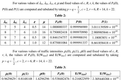
For various values of λ01, λ02, λ12, ε, µ and fixed values of c, R, r, k, the values of P0(0),

P(0) and P(1) are computed and tabulated by taking p = q = 1

2, c = 2, r = 6, R = 14, k = 22. Table 2:

λλλλ01 λλλλ02 λλλλ12 εεεε µµµµ P0(0) P(0) P(1)

7 5 4 0.5 14 1.000000337 0.999996989 3.011139509 × 10-06 8 7 6 1.0 16 0.750002418 0.999970990 2.900985846 × 10-05 9 7 6 0.5 18 0.846154757 0.999988191 1.18083851 × 10-05 6 5 4 1.0 12 0.875001084 0.999991337 8.661858418 × 10-06

For various values of traffic intensities ρ1(0), ρ1(1), ρ(0) and fixed values of c, R,

r, k, the values of P0(0), E(WEle0) and E(WEle1) are computed and tabulated by taking

p = q = 1

2, c = 2, r = 6, R = 14, k = 22.

Table 3:

ρρρρ1(0) ρρρρ1(1) ρρρρ(0) P0(0) E(WEle0) E(WEle1) 0.9629629 0.8148148 1.6296296 0.538482476 0.216822959 2.305440288 × 10-04 0.9333333 1.0666666 1.7333333 0.571168139 0.191642350 1.954836409 × 10-04 0.9714285 0.8571428 1.7142857 0.529430081 0.168165285 2.048172575 × 10-04 0.9090909 1.0909090 1.6363636 0.599981582 0.257493967 2.047189430 × 10-04

For various values of traffic intensities ρ2(0), ρ2(1), ρ(0) and fixed values of c, R,

r, k, the values of P0(0), E(WEme0) and E(WEme1) are computed and tabulated by taking

p = q = 1

2, c = 2, r = 6, R = 14, k = 22.

Table 4:

ρρρρ2(0) ρρρρ2(1) ρρρρ(0) P0(0) E(WEme0) E(WEme1) 0.6666666 0.5185185 1.6296296 1.000000337 0.407405101 2.672235613 × 10-06 0.8000000 0.6666666 1.7333333 0.750002418 0.344406862 3.873679121 × 10-05 0.7428571 0.6285714 1.7142857 0.846154757 0.301889433 8.168855381 × 10-06 0.7272727 0.5454545 1.6363636 0.875001084 0.483755854 3.944311137 × 10-06

24

From Tables 1 and 2 the following observations can be made:

i. In the long run, the probability that the system to be in the faster rate of arrivals either with feedback or without feedback is nearly unity. But the probability that the system to be in the slower rate of arrivals either with feedback or without feedback is very small.

ii. When the system is in the faster rate of arrivals either with feedback or without feedback, the probability that the system size is zero decrease when the arrival rate of the Elective customers or the arrival rate of the Emergency customers increases.

From Tables 3 and 4 the following observations can be made:

iii. Either the system is in the faster rate of arrivals or in the slower rate of arrivals either with feedback or without feedback, the expected waiting time of Elective customers [E(WEle0)] and the expected waiting time of emergency customers

[E(WEme1)] increase as the parameters ρ1(0) and ρ2(0) increases.

iv. When the system is in the faster rate of arrivals either with feedback or without feedback, the expected waiting time of Elective customers [E(WEle0)] and the

expected waiting time of Emergency customers [E(WEme0)] decrease as the traffic

intensities ρ1(0) and ρ2(0) increases.

v. When the system is in the slower rate of arrivals either with feedback or without feedback, the expected waiting time of Elective customers [E(WEle1)] and the

expected waiting time of Emergency customers [E(WEme1)] increase as the traffic

intensity ρ1(1) and ρ2(1) increases.

REFERENCES

1. D. Gross and C.M. Harris, Fundamentals of Queueing Theory, John Wiley, New York, 1974.

2. D. Gross and C.M. Harris, Fundamentals of Queueing Theory, Third Edition, Wiley Intersciences, New York, 1998.

3. R. Kalyanaraman and S. Sumathy, A Feedback Queue with multiservers and Batch Service, International Review of Pure and Applied Mathematics, 5(1) (2009) 23-27. 4. J. Medhi, Stochastic Models in Queueing Theory, 2/e Academic Press, An imprint of

Elsevier, 2006.

5. G. Rani and A. Srinivasan, M/M/c/k Interdependent Queueing Model with controllable Arrival Rates and feedback, IJAMAA, 7(2) (2012) 131-141.

6. G. Rani and A. Srinivasan, M/M/c/k Loss and Delay Interdependent Queueing Model with controllable Arrival Rates, No passing and Feedback, International Journal of Mathematical Sciences and Engineering Applications, 7(IV) (2013) 403-419.

7. A.Srinivasan and M. Thiagarajan, A finite Capacity multi-server Poisson input Queue with Interdependent inter-arrival service time and controllable arrival rates, Bulletin of Calcutta Mathematical Society, 99(2) (2007) 173-182.

8. V. Thangaraj and A. Shanthakumaran, A Queue with Markovian feedback, Int. Jr. of Infor. and Manage, Sci., 6(4) (1995) 35-45.