Entrepreneurial effort and economic growth

R E S E A R C H

Open Access

Entrepreneurial effort and economic growth

Félix-Fernando Muñoz

and Francisco Javier Otamendi

* Correspondence:

felix.munoz@uam.es 1_{Departamento de Análisis}

Económico: Teoría Económica e Historia Económica, Universidad Autónoma de Madrid, C/ Francisco Tomás y Valiente 5, Madrid 28049, Spain

Full list of author information is available at the end of the article

Abstract

Entrepreneurs allocate resources among different activities that generates a profit; in particular, in this paper entrepreneurs consider at each instant of time both innovation and rent-seeking as alternative sources of profit. The consequences in terms of economic growth are obviously quite different: the higher the amount of innovations in the economy the higher the rate of economic growth and vice versa. What are the determinants of these different entrepreneurial behavior? Is there anything in the nature of entrepreneurs that essentially distinguishes between innovators and rent seekers? A main claim of this paper is that differences among entrepreneurs are not essential but of degree: all of them are in fact profit-seekers and the only difference is to be found in their attitude towards innovation as a source of profit. In this sense entrepreneurial effort is defined and modelled for each entrepreneur according to its propensity to innovate and the corresponding Entrepreneurial Problem (EP) is posed and solved both analytically and via simulation in terms of profit maximization. The individual decisions measured in units of innovation are then aggregated to calculate the innovation quantity for a given population based on the distribution of heterogeneous entrepreneurs. The entrepreneurship rate and the implications for economic growth are also modelled. Consequently, policy makers should focus on reducing the entry barriers and the costs of production in order to stimulate the entrepreneurial activity and maximize the innovation quantity.

Keywords:Entrepreneurial heterogeneity; Propensity towards innovation; Allocation of entrepreneurial effort; Endogenous growth

Background

In a letter to F.A. Walker, Léon Walras claimed that the definition of entrepreneur was, under his point of view,“le nœud de toute l’économique”(Walras 1965). Entrepreneurship plays a fundamental role in the explanation of many economic phenomena, but at the same time there must exist few central economic concepts that have been understood and applied in such a diverse manner (Casson 1982, 1987; Casson et al. 2006). Thus, the entrepreneur is the agent who, in the search for profit, coordinates the markets–this is the case of Walrasian and neoclassical economics and, in a very especial sense, Austrian economics (Kirzner 1992)-; introduces new combinations in the economic life (Schumpeter (1932) [2005]; Schumpeter (1934) [1983]; assumes the risks involved in all the decisions that are taken in contexts of true uncertainty (Knight 1921); etc. In any case, economists agree on that the main contribution of the entrepreneur within the economy consists of increasing the productivity of the system through innovation. Moreover, it is pursuing their own interest (profits) that entrepreneurs coordinate and enhance the productivity of the economy thus promoting economic growth.

However, the hypothesis that entrepreneurs just behave as profit maximizers does not exclude other sources of profit for entrepreneurs. In fact, as overwhelming evidence from economic history suggests, rent-seeking may be considered also as an entrepre-neurial activitya. In this case, their activity consists mainly of pursuing the maximum possible profits not linked to innovations or activities that generate productivity gains. By behaving in such a manner, depending on their capacity to absorb resources of the economy, this type of entrepreneurship may end up rationing scarce resources required by the innovator-entrepreneurs to develop their activities; i.e.: rationing the necessary resources that will truly promote increases in productivity of the economy in the long term (Acemoglu and Robinson 2012; Murphy et al. 1991, 1993).

How can be these alternative uses of entrepreneurial capacity–and their different conse-quences in terms of economic growth- be integrated in a single model without assuming that innovative entrepreneurs and rent-seeking entrepreneurs are essentially different? Departing from Baumol (1968) seminal work, we develop a quite simple idea in order to link different entrepreneurial activities under a single“entrepreneurial problem”. We do so by introducing entrepreneurial heterogeneity by assuming that entrepreneurial activities may be any combination of the two extreme kinds: innovative and rent-seeking. However, contrary to Baumol’s claim that“no exhaustive analysis of the process of allocation of entre-preneurial activity among the set of available options will be attempted”and therefore“only at least one of the prime determinants of entrepreneurial behavior at any particular time and place is the prevailing rules of the game that govern the payoff of one entrepreneurial activity relative to another”(Baumol 1990, 898, emphasis in the original), we model differ-ent differ-entrepreneurial activities without assuming that differ-entrepreneurs areessentiallydifferent, and explore the implications of different structures of payoffs over innovation activities.

For doing so, we introduce as a characteristic or each entrepreneur an attitude or propensity towards innovationand distribute it among a (theoretical) population of en-trepreneurs. Thus, we define an entrepreneurial distribution function between the two extremes–pure innovators and rent-seekers-, a function that captures thehypothesis of heterogeneity of entrepreneurs. The distribution of entrepreneurs’ attitude towards innovation consists of assuming that each entrepreneur in the economy establishes the relative value of each of the two extreme types together with the restrictions that im-pinge upon these values. Next we assume that each (heterogeneous) entrepreneur max-imizes his utilityfunction associated to innovation opportunities and the possibility of obtaining economic rents, subject to a minimum level of (subjective) profits. Given the entrepreneur’s attitude towards innovation, and depending on the availability of alterna-tive earnings within the economic system (rents), he decides how many resources they will devote to innovation, taking also the entry barrier costs into account. Formally, the entrepreneurial problem (EP) could be then stated as follows for each entrepreneur:

Max: Utility due to entrepreneurial effort

s.t. profit is at least enough to compensate entry barrier costs in innovation and alternative sources of gains (rents)

entrepreneurs and the overall quantity is included into the growth model to derive po-lice implications. The rate of entrepreneurship is also calculated as a by-product.

Methods

In order to characterize each entrepreneur, we describe the two extreme types of atti-tudes towards innovation that frame the strategies of the individuals:

(a) type 0, entrepreneurs associated with pure innovative activities

(b) type 1, entrepreneurs whose underlying (and unique) objective is the search for the maximum possible source of earnings–rents- in the economy.

By doing so, each entrepreneur might be represented by his specific position between the two extremes: his relative position is defined by δ ∈[0,1]. Therefore, by construc-tion, δ is both the propensity and the “psychological distance” of any given entrepre-neur from the extreme type 0 –being an innovator. Consequentially, (1 - δ) is the

“psychological distance”from type 1–being a rent-seeker. Each entrepreneur has there-fore two ways of obtaining utility gains: via pure innovation; and via economic profit, which may be obtained either by innovating or by other alternative activities such as rent-seeking. How each entrepreneur weighs exactly each possibility of improving his personal situation is described by his propensity to innovate,δ.

Each entrepreneur δ must first decide how much of the innovative good he would produce, should he choose to produce it at all, and then he must decide which activity he will finally opt for. Let q(δ) be the amount of innovation that an entrepreneur of type δ will produce under the assumption that an invention is availableb. In other words,q(δ) is the effort towards innovation that an individual entrepreneur allocates.

Whenever facing the allocation problem, the entrepreneur will then have to decide between:

(a) producing a positive quantity of the innovative good,q(δ) > 0

(b) obtaining a“rent”by carrying out other activities in some other sector of the economy; in this caseq(δ) = 0.

The objective function: utility gains

To decide on how to allocate the innovation effort among the different alternatives, the ob-jective of a given entrepreneurδis defined in terms of asubjective utility functionthat mea-sures the degree in which the entrepreneur takes part in activities of type 0 and of type 1.

Uðδ;qÞ ¼ð1−δÞu qð Þ þδvðπð Þq Þ ð1Þ

The economic profit associated with the quantity of innovative good produced, q, is defined by:

πð Þq ≡ðp qð Þ−cÞq ð2Þ

wherep(q) is the demand function for the innovative good; andcis the average cost as-sociated with the production of an additional unit ofq.

The binding restriction: the necessary condition to innovate

Although maximizing profits, no entrepreneur would want to become bankrupt by car-rying out the innovative activity that he values most. He will always search for a satis-ficing earning that is at least equal to the cost of innovating, α0, should he decide to repeat his plan in the future. The entrepreneur will then compare this earning, from his position δ, with his other options, the non-innovation rents, denoted by R. This minimal condition to innovate may be defined as follows:

p qð Þ−c

ð Þq¼πð Þq

½ ≥½αð Þ ¼⋅ α δð ;α0;RÞ ð3Þ

whereα(·) is a function that sets the minimum yield (satisficing threshold) that the plan of each typeδentrepreneur must obtain. This functionα(·) has as arguments:

(1) the propensity of the entrepreneur towards innovation,δ (2) the cost of introducing an innovation or entry barrier,α0

(3) the gains that can be obtained in other sectors of the economy,R. (This last variable together withπ(q) represent the structure of payoffs of the economy.)

In order to innovate, that is, forq(δ) > 0, it must happen that, the minimum condition π(q)≥α(·) is satisfied. If it is not satisfied for the corresponding values ofα0andR, the entrepreneur chooses not to innovate in new goods, q(δ) = 0, and engages in rent-seeking activities.

The entrepreneur’s problem (EP)

We may then formally set the “allocation of entrepreneurial effort” problem as follows after consistently combining the type of entrepreneurship, the decision variable, the objective function and the binding restriction:

EP

ð Þ: (

max

q≥0 Uðδ;qÞ ¼ð1−δÞu qð Þ þδvðπð Þq Þ s:t:: πð Þq ≡ðp qð Þ−cÞq≥α δð ;α0;RÞ

ð4Þ

Results and discussion

The allocation of entrepreneurial effort

The decision that each economic agent should take concerning the allocation of the entrepreneurial effort depends therefore onα0,R, c, p, and δd; although the (EP) solu-tion for each particular entrepreneur δ exists and it is uniquee. We denote this optimum innovation quantity by:f

For any solution regime, if any of the influential parameters are separately evaluated for sensitivity, it can be shown thatg:

∂q ∂α0<

0; ∂q

∂R<0; ∂q ∂c<0;

∂q ∂p>0;

∂q

∂δ<0 ð6Þ

In words, the quantity of innovation goods generated by the solution of (EP) is higher:

(1) the lower the minimum profit claimed by entrepreneurs in innovative activities,α0;

(2) the lower the alternative sources of gains,R; (3) the lower the cost of producing innovations,c; (4) the higher the price of innovations,p;

(5) the higher the individual propensity to innovate, that is, the lowerδ.

These statements look intuitive if taken one-at-a-time. However, if all the effect are jointly considered and analyzed, we may summarize the decision possibilities faced by the entrepreneur as follows: (a) there will never be innovation if the entry barrier cost is higher than the profit, regardless of the entrepreneurial type and the propensity to innovate; (b) there will always be innovation if the profit is higher than the alternative rent, regardless of the entrepreneurial type; and (c) otherwise, some entrepreneurs might innovate, depending on where the value of the profit lies with respect to the entry barrier and the rents.

Entrepreneurship and economic growth: some policy implications

The aggregate behavior of the economy depends on how, not the individual entre-preneurs allocate their efforts according to the (EP), but all of the entrepreneurs jointly carry out their activities. Different social structures of payoffs (Baumol 1994) will result in different economic performances (in terms of growth of output, for example) through the different ways to allocate the efforts of innovation of the entrepreneurs. The internal evolution of the social dynamics also determines the distribution of entrepreneurs within a given economy between the two extreme types.

Modern endogenous growth models in economy stress the deep relationship that ex-ists between entrepreneurship and the economic performance of a society as measured for example by the per capita output growth (Acemoglu 2009). The answers provided by economic growth theory are rather varied, ranging from models that abstract entre-preneurial activity (see for example Mankiw et al. (1992), Solow (1956) to those that formally integrate entrepreneurship into models that incorporate the intentional actions of entrepreneurs in the explanation of how the rate of growth is determined (Aghion and Howitt 1998; Romer 1994).

Aggregate innovation effort

The aggregate value of innovation for the economy as a whole, Q, is determined by adding the individual quantities of innovation across all the entrepreneursδ. Thus:

Q¼

Z 1

0

qð Þδ fð Þδ dδ ð7Þ

Let us denote byf(δ) the density function of the propensity to innovate, in order to characterize any given economy. A higher propensity of society towards innovation is captured in the model by a “higher” density of entrepreneur propensity to innovate. The shape of this last “variable” f (δ) may differ drastically between economies–both between different contemporaneous economies and the same economy at different timesh.

The economic policy efforts should then be based on the maximization of not only the individual entrepreneurship activities, q*, but also on the distribution of the pro-pensities f (δ) in order to increase the number of entrepreneurs; that is, politicians should foster that entrepreneurs shift their propensity towards pure innovation (1−δ), lowering their individualδ.

Entrepreneurship rate

From the solution of (EP) it is also possible to directly define and calculate an index that refers to the rate of innovative entrepreneurs of a given economy. We define the entrepreneurship rate as δ0. Its value, which ranges between 0 and 1, is calcu-lated by solving:

πmax¼α αð 0;R;δ0Þ ð8Þ

Those entrepreneurs with 0≤δ≤δ0 will allocate efforts to entrepreneurial activities since their propensity to innovate δ is close enough to pure innovation (δ= 0), while those with higher values ofδwill not as they are closer to rent-seeking (δ= 1). The eco-nomic implications of this index are that policies centered in ecoeco-nomic growth should strive for lowering both the entry barriers and the other rents of the economy and to increase the profit associated to innovation.

Economic growth

In order to study how the aggregate allocation of the entrepreneurial efforts affects the dynamics of the economy, we use an adapted version of Rivera-Batiz and Romer (1991) endogenous growth model for evaluating the evolution of the rate of change of innovations over time, denoted by γy. According to this model, the rate of change of

innovations is:

γy¼

1−μ ð ÞβQ−Qc_

QC−α0

ð9Þ

where we assume a consumption function C=μYwith a constant marginal propensity to consume 0 <μ< 1; andβis the productivity of the innovationi.

inversely proportional to the cost of developing and producing them, and in the pro-duction of existing goods. Once again, entry barriers and costs should be lowered, whereas productivity should be increased.

These statements perfectly fit into the framework of the individual (EP), giving consistency to the overall approach of this research that relates the allocation of innovation effort by heterogeneous entrepreneurs and the growth of the economy.

A numerical illustration

The (EP) model is both solvable analytically and by means of simulation techniques. Next we propose to solve a theoretical example. For the sake of simplicity, let us use linear functions and the following input values:

(a) p(q) =a−bq, witha,b> 0 (b)u(q) =dq, d> 0

(c)vðπð Þq Þ ¼q

(d)α δð ;α0;RÞ ¼ð1−δÞα0þδR

The formulation of the (EP) for each entrepreneur is then the following:

EP

ð Þ: maxq≥0 Uðδ;qÞ ¼du qð Þ þδπð Þq

s:t:: πð Þq ≥α δð ;α0;RÞ ¼ð1−δÞα0þδR (

ð10Þ

Analytically, the solution is given by:

qðδ;α0;RÞ ¼

minfq₁ðδ;RÞ;q₂ðδ;RÞg ifα δð ;RÞ≤ða−cÞ 2

4b

0 ifα δð ;RÞ>ða−cÞ 2

4b

8 > > < > >

: ð

11Þ

Where

q1¼ a−c

ð Þ

2b þ

ffiffiffiffiffiffiffiffiffiffiffiffiffiffiffiffiffiffiffiffiffiffiffiffiffiffiffiffiffi

a−c

ð Þ2₋ 4bαð Þ⋅

q

2b

q₂¼ða−c−dÞ

2b þ

d

2bδ

ð12Þ

The entrepreneurship rate (δ0) follows:

δ0¼ a−c

ð Þ2 4b −α0

R−α0

ð13Þ

We proceed to further assign numerical values to the input variables:

R= 0.33

_a= 5;b= 6.67; sop(q) = 5–6.67q

c= 2.75

d= 0.20;u(q) = 0.20q

Figure 1 shows the quantity of innovation for each entrepreneur as a function of the distance δ to pure innovation. The theoretical break point or entrepreneurship rate is at δ0= 0.5617 for any f(δ). It also shows that the quantity is calculated from function q1ifδ< 0.091 and from functionq2if 0.091 <δ< 0.5617.

However, even in this simple case, it is not straightforward to calculate the amount of innovation in the economy, because it is very complex to integrate Qdue to the exist-ence (at least a priori) of non-linearities in the model and due to the shape off(δ). For the specific case of the Uniform distribution, U(0, 1), the average of the quantity of innovation isQ* = 0.1293.

Concerning the growth of the economy, if the propensity to consume is μ= 0.8 and the productivity isβ= 1.5, the rate of innovation isγy= 10.91%.

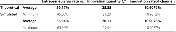
The allocation problem is also simulated both to validate the analytical solution and also to assess variability in terms of the number of entrepreneurs in the populationj. ForN= 200 entrepreneurs, 50 simulations are run. The main results are that the quan-tity of innovation in the economy,Q*, lies between 21.2820 and 29.4426 with an aver-age of 26.1124 (its theoretical value is Q* = 25.8557); the rate of entrepreneurship, δ0, lies between 45% and 65.5% with an average of 56.54% (its theoretical value is δ0= 56.17%); and the rate of change of the economy, γy, lies between 10.9272% and

10.9277% (its theoretical value isγy= 10.9276%).

Conclusions

In this paper we consider that entrepreneurial activities range from innovation to rent-seeking. This assumption allows us to link both innovation and rent-seeking in a uni-tary formal framework of entrepreneurship. From (EP) it is possible to establish the re-lationship between variables such as minimum profit threshold (a version of the satisfying behavior hypothesis (Cooper 2003, 26); opportunity of gains in other sectors of the economy (Baumol’s structure of payoffs); the costs of innovation; and the quan-tity of innovation finally produced depending on the attitude of entrepreneurs them-selves and society in general towards innovation effort -defined by f(δ) -, and the consequences of their joint study in the rate of growth of economic output.

In the allocation of effort (EP) problem, each entrepreneur δ compares the potential earnings associated with the production of the innovative good q*, with an alternative source of earnings linked to rent-seeking activities, R. If the minimum condition to innovate is not satisfied, the entrepreneur choosesnot to introducenew goods and engages in rent-seeking activities. The formal problem is an illustration of how the entrepreneur faces the dilemma of how to allocate the scarce resources to which he has access with the intention of getting what he esteems it should be a gain high enough linked to his activity.

The (EP) problem is solvable both analytically and by means of simulation tech-niques. In fact, simulation is a reliable option whenever analytical solutions are diffi-cult to obtain. A validation exercise has been carried out using linear functions in order to provide an illustration of how the model works. A natural extension of (EP) would consist of parameterizing the input variables, specifically the entrepreneurial functionf(δ), and performing a robust study of the behavior of the model with ad-hoc simulations.

The solution of (EP) establishes a relationship between the quantity of innovation for each entrepreneur as a function of the distance δ to pure innovation and rent-seeking. It also allows for the definition of an entrepreneurial index that quantifies the proportion (δ0) of innovative entrepreneurs of a given economy. Entrepreneurs within the interval 0≤δ≤δ0 will innovate and those with higher values of δ will not.

The implications on economic growth follow. Policy makers should implement pol-icies that reduce the opportunity costs of innovation, R, as well as the entry barrier costs, α0; the direct costs of production of innovations (for example subsidizing innovation activities), c; and promoting an innovation culture that shapes the propen-sity to innovation distributionf(δ) in favor of innovative activities.

Endnotes

a

b

This amount may refer to a new investment good (capital) (Romer 1990) or to an existing one but with new features that makes it more productive (Grossman and Helpman 1991).

c

Note that the first term always refers to the utility obtained from innovating. d

For simplicity, we have set α0and R as constants and equal for all entrepreneurs, identical for all types of innovations. The same assumptions can be applied to the aver-age costs of production of an additional unit of the new good,c.

e

The continuity of the utility function and the fact that the feasible set is closed and bounded guarantees that there exists a global maximum (Weierstrass Theorem). More-over, since the function is strictly concave and the feasible set is convex, the Fundamen-tal Theorem of Convex Programming guarantees that the global maximum of (EP) is unique.

f

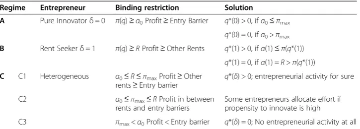
The different regimes of solution are summarized in Table 1 and their mathematical derivation is included in Appendix I.

g

See Appendix III. h

The main results are summarized in a formal proposition in Appendix I and the proofs are included in Appendixes III and IV.

i

For more details, see Appendix V. j

For a description of the pseudocode of the simulation model see Muñoz and Otamendi (2012).

k

We apply the Kuhn-Tucker conditions. l

See Appendix II for a formal proof. m

See Appendix III. n

We say “decreasing” rather than the partial derivative is negative, since there exist points at which the functions are not differentiable. Since they are continuous, the form of the relationship is maintained.

o

For a proof of this proposition, see Appendices III and IV. p

See Appendix IV.

Appendix I: regimes of solution for (EP)

We assume that u′,v′> 0 andu″,v″≤0;π″< 0; the marginal cost is positivec> 0;δ∈ [0, 1]; R≥α0> 0 ; the demand for innovative products is p(0) >c; and there exists a q^ such thatp(q) = 0, for allq≥^q andp′(q) < 0 for allq<q′; the properties of the threshold function are α′_δðδ;α0;RÞ>0, α′α0ðδ;α0;RÞ>0, α

′

Rðδ;α0;RÞ>0; and the two extreme cases are α(0,α0,R) =α0and α(1,α0,R) =R. From the assumptions on the demand for new goods, there exists a q~∈ð0;q^Þ such thatpð Þ ¼q~ c. Therefore,πð Þ ¼0 π~ð Þ ¼~q 0. Fi-nally, from the concavity of the profit function follows that there exists a global max-imum of π(q), q∈½0;q~. Hence, it holds that π′(q) > 0 if 0≤q≤q; and π′(q) < 0 when

Table 1 Results of the simulation

Entrepreneurship rateδ0 Innovation quantityQ* Innovation rateof changeγ

Theoretical Average 56.17% 25.85 10.9076%

Simulated Minimum 45.00% 21.28 10.9072%

Average 56.54% 26.11 10.9076%

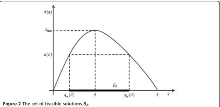
q≤q≤~q. This result -together with the functionα(·) - determines the feasible set for each δtype entrepreneur.

From the functions π(q) andα(·), the feasible set for each typeδentrepreneur,B_δ, is determined byB_δ= {q∈ℝ/π(q)≥α(δ,α0,R)}. Figure 2 represents this set.

For each value ofπ(q) andα(•) there are two possibilities:

πð Þq ≥α ifα>πmax;thenBδ ¼∅

ifα≤πmax;thenBδ≠∅

(

ðAI:1Þ

In the second case, the feasible set is determined by the interval:

Bδ¼½qmð Þδ ;qMð Þδ ðAI:2Þ

The continuity of the utility functionU(δ,q) and the fact that the feasible set is closed and bounded guarantees that there exists a global maximum (Weierstrass Theorem). Moreover, sinceU(δ,q) is strictly concave and the feasible set is convex, the Fundamen-tal Theorem of Convex Programming guarantees that the global maximum of (EP) is unique. We denote this maximum byq*(δ).

Innovation regimes whenBδ≠ ∅

In the most interesting and general case there are two possibilities: (a) that the solution to (EP) is strictly interior, and (b) the solution lies on the frontier of the feasible setk. If the solution isinterior, then it must hold that the optimalq*(δ) is that which maximizes type δ entrepreneur’s utility (for λ= 0); i.e.: a value of q such that (1−δ)u′(q) +δv′ (π(q))π′(q) = 0. Equivalently, the condition that must be satisfied is:

v′ðπð Þq Þπ′ð Þq u′ð Þq ¼

1−δ

δ

ðAI:3Þ

In this condition the left-hand-side term may be interpreted as some type of marginal rate of substitution between innovations and profit that depends on the relative pos-ition of each entrepreneur in the distributionf(δ). On the other hand, the frontier solu-tion applies when π(q) >α(δ). In this second case, the solution is given by the restriction of (EP). In principle, this solution could be at eitherq* =qm(δ) orq* =qM(δ).

From the condition L′_q ¼0, and from the hypotheses on the functions of the problem,

it holds thatπ′(q*) < 0, and so the solution is given byq*(δ) =qM(δ).

Another interesting feature of this model is that it generates a change in the solution regime when the solution passes from interior to binding or vice versa. This asymmet-ric behavior (some entrepreneurs behave like type 0s, while other like type 1s) is quite logical given the special functional form that has been assumed for the general utility function of the entrepreneurs,U(δ,q), i.e.: a linear combination of the two extreme, or pure, types of behavior. There is exactly one (or some) intermediate value that weighs the two parts of the utility function equally. (Appendix III provides the formal proof.)

Comparative statics

From Eq. (5), it is possible to analyze the relationships between the solution of the amount of innovation and the other arguments of the function. An unusual characteris-tic of (EP) solution is that it appears inzoneswithin the distribution, which implies that these partial relationships within each zone must be considered, bearing in mind at all times the points at which one regimen of solution joins another. These joining points

take place at the valuesδ^that satisfy the following conditionl:

H qð _Mð Þδ Þ<− 1−δ δ

ðAI:4Þ

In any case, it can be shown for both solution regimes (interior and frontier) thatm:

∂q ∂α0<

0; ∂q

∂R<0; ∂q ∂c<0;

∂q ∂p>0;

∂q

∂δ<0; ðAI:5Þ

Consequentially, given the functional relationships that have been assumed for de-mand, utility, variable costs, attitude towards innovation and the profit restriction, etc., the relationship q*(δ) =q(δ,α0,R,c,p) isdecreasingnin the position of the entrepreneur in the entrepreneurial capacity distribution, δ, in the economic cost of developing in-ventions, α0; in the rents available within the economic system,R; and in the variable production cost associated with innovations, c. Obviously, there is a positive depend-ence on the demand for innovative goods. That is, the closer is an entrepreneur (psy-chologically) to being of type 1 (i.e.: values profits relatively more), the greater isR; the greater is the cost of production of innovations (a usual argument for subsidizing innovation activities); and the greater the unitary production costs are; the lower the in-novative activity of entrepreneurs as measured by q will be. The following proposition resumes the main results.

Proposition: There exists a single solution to (EP) for eachδ, denoted by q*(δ) =q* (δ,α0,R,c,p) that is continuous (except at the point ~δ whenever this is not greater than 1) on the interval [0, 1], that is differentiable at almost all points. Moreover, the

aggre-gate solution of (EP),Qð Þ ¼δ

Z 1

0

qð Þfδ ð Þdδ δ is decreasing inα0,Randc, and

increas-ing infandpo.

Appendix II: switching point

H qð Þ ¼v

′_{ðπð Þq Þπ}′_{ð Þq}

u′ð Þq ðAII:1Þ

We have Hð Þ ¼q 0 andH is strictly decreasing since H′(q) < 0. Therefore, the solu-tion is interior if and only if

H qð _Mð Þδ Þ<− 1−δ δ

ðAII:2Þ

In case (C.1) and in those cases of (C.2) in which the B_δ≠ ∅(see Table 2), these two

innovation regimes are operative. Moreover, there exist some values δ^ for which these

regime changes will occur. For these δ^ there will be an“inflection”(or connection) be-tween the two types of solution. At these solutions it must hold that:

H qð Mð Þδ Þ ¼−

1−δ

δ qð Þ ¼δ q_Mð Þδ

that is; ^δ¼

v′ðπðqð Þδ ÞÞπ′ðqð Þδ Þ u qð ð Þδ Þ ¼−

1−δ

δ

πðqð Þδ Þ ¼α δð Þ

8 < : 8

<

: ðAII:3Þ

Appendix III: comparative statics

Consider q*(δ) =q(δ,α0,R,c,p). We have to distinguish between interior and frontier solutions.

Derivatives with respect toδ.

Interior solution.

v′ðπðqð Þδ ÞÞπ′ðqð Þδ Þ u qð ð Þδ Þ ¼−

1−δ

δ

ðAIII:1Þ

From which

q′ð Þ ¼δ u

′_{ðqð Þδ Þ−v}′_{ðπðqð Þδ ÞÞπ}′_{ðqð Þδ Þ}

δv″ðπðqð Þδ ÞÞðπ′ðqð Þδ ÞÞ2þδv′ðπðqð Þδ ÞÞπ″ðqð Þδ Þ þð1−δÞu″ðqð Þδ Þ<0

ðAIII:2Þ

Table 2 Summary of results

Regime Entrepreneur Binding restriction Solution

A Pure Innovatorδ= 0 π(q)≥α0Profit≥Entry Barrier q*(0) > 0, ifα0≤πmax

q*(0) = 0, ifα0>πmax

B Rent Seekerδ= 1 π(q)≥RProfit≥Other Rents q*(1) > 0, ifα(1)≤π(q*(1))

q*(1) = 0, ifα(1) =R>π(q*(1))

C C1 Heterogeneous α0≤R≤πmaxProfit≥Other rents≥Entry barrier

q*(δ) > 0; entrepreneurial activity for sure

C2 α0≤πmax≤RProfit in between

rents and entry barriers

Some entrepreneurs allocate effort if propensity to innovate is high

Frontier solution: we begin withπ(q(δ)) =α(δ). Hence,

q′ð Þ ¼δ α ′_{ð Þα}

π′_{ðqð Þδ Þ}<0 ðAIII:3Þ

Note: we have discussed several solution regimes, which implies that one of them could be repeated. But in any case, the dependence is inverse (negative). On the other hand, it may well happen that, beginning with a particular value of δ the solutions

“jump” to zero. We have not studied these cases since the solution is to always have zero innovations

Derivatives with respect toR.

Interior solution. Since the entrepreneur’s restriction is constant inRfor each interior value ofδ, changes inRdo not directly affectq*in this case. There is, however, an in-direct effect, since Rdetermines the value of the function α(•), and sinceα(•) defines the setB_δ, changes inRwill alter the values ofδthat determine the changes in solution regime.

Frontier solution. In this case, R has a direct effect on the restriction through the functionα(•). Hence, sinceπ′(q(R))q′(R) =α′(R), we have

q′ð Þ ¼R α ′_{ð ÞR}

π′_{ðq Rð ÞÞ}<0 ðAIII:4Þ

Derivatives with respect toc.

Interior solution. Beginning with (1−δ)u′(q(c)) +δv′(π((c,q(c))))π′(c,q(c)) = 0, taking π=π(c,q),π′¼∂_∂π_q and since∂_∂π_c−q, together with the fact thatp″(q(c))q(c) + 2p′(q(c)) =π″ (q(c)), we may conclude that

q′ð Þ ¼c qδv

″_{ðπðc;q cð ÞÞÞπ}′_{ðc;q cð ÞÞ þδv}′_{ðπðc;q cð ÞÞÞ}

δv″ðπðc;q cð ÞÞÞðπ′ðc;q cð ÞÞÞ2þδv′ðπðc;q cð ÞÞÞπ″ðc;q cð ÞÞ þð1−δÞu″ðq cð ÞÞ<0

ðAIII:5Þ

Frontier solution forπ=π(c,q(c)) =α(·)

q′ð Þ ¼c q

π′_{ðc;q cð ÞÞ}<0 ðAIII:6Þ

Dependence onp.

An additional problem is that of the dependence of q on changes in the demand func-tion,p(q). In this case the dependence is with respect to a function, which makes it im-possible to evaluate, although it is clear that greater demand will imply greater profit opportunities and, additionally, greater incentives to produce greater amounts of in-novative goods.

Appendix IV: stochastic dominance

it depends on a characteristic of the distribution functions with very little a priori in-formation -, it is possible to establish one important result: the average level of innovation in the economy -as measured from (9)- is greater in those economies whose entrepreneurial capacitydistribution function first order stochastic dominates another. That is, given two different entrepreneurial capacity density functions,f1and

f2, where we defineFið Þ ¼δ Z δ

0

f_ið Þdss , fori= 1, 2, if it holds that

F1ð Þδ ≥F2ð Þδ ;∀δ∈½0;1 ðAIV:1Þ

then we haveQ1≥Q2, for given values of the other variablesp. Graphically, distribution

f1 first order stochastic dominates f2 if their relative positions are as represented in Figure3.

If we denoteQ1−Q₂¼

Z 1

0

qð Þδ ðf₁ð Þδ −f₂ð Þδ Þdδ and integrate by parts, then

Q₁−Q₂¼qð Þδ ðF1ð Þδ −F2ð Þδ Þj10− Z 1

0

q′ð Þδ ðF1ð Þδ −F2ð Þδ Þdδ

¼−

Z 1

0

q′ð Þδ ðF1ð Þδ −F2ð Þδ Þdδ>0 ðAIV:2Þ

we have thatQ1≥Q2.

Appendix V: growth model

We assume the following definition of capital:

K tð Þ ¼A tð ÞQ tð Þ ðAV:1Þ

whereK(t) is the accumulated amount of goods that have been incorporated in the pro-duction process, andA(t) is the number of varieties of new production goods that have been generated up to the moment of time t. That is to say, at each moment t, the amount of varieties that can be used in the production of output is given by the amount (and number) of innovative goods of previous periods, as well as those that are introduced at momentt. Hence, the introduction of new goods will imply an increase

(change) inA(t) equal toA t_ð Þ; andA(t) will depend on both the dynamics of inventions and the dynamics of innovations.

In fact:

γy¼γA¼

_

A A¼

1−μ ð ÞβQ−Qc_

QC−α0

ðAV:2Þ

In the Rivera-Batiz and Romer model, changes inAare denoted as:A_ ¼τHA; that is, the rate of growth of Ais proportional to the human capital in the system, H, and a parameter that measures the productivity of this capital, τ. In these types of model, it also turns out that all inventions are introduced into the economic system as innova-tions. In our case, things do not happen with such a high degree of automation, since the entrepreneurs, from the problem (EP) and their relative types,δ, will determine the amount of each invention (variety) that will be produced, where a possible solution is that no positive amount at all is produced, i.e.: an invention is not transformed into an innovation.

Competing interests

The authors declare that they have no competing interests.

Authors’contributions

FFM designed the model. FJO simulated the model and analyzed results. FFM and FJO wrote the paper. All authors read and approved the final manuscript.

Author details

1_{Departamento de Análisis Económico: Teoría Económica e Historia Económica, Universidad Autónoma de Madrid,}

C/ Francisco Tomás y Valiente 5, Madrid 28049, Spain.2Departamento Economía Aplicada I, Universidad Rey Juan Carlos, Paseo Artilleros s/n, Madrid 28032, Spain.

Received: 31 March 2014 Accepted: 21 April 2014 Published: 18 June 2014

References

Acemoglu, D (2009).Introduction to modern economic growth. Princeton: Princeton University Press. Acemoglu, D, & Robinson, JA (2012).Why Nations Fail: The Origins of Power, Prosperity, and Poverty. New York:

Crown Publishers.

Aghion, P, & Howitt, P (1998).Endogenous Growth Theory. Cambridge, MA: The MIT Press.

Arezki, R, & Brückner, M (2010).Commodity Windfalls, Polarization, and Net Foreign Assets: Panel Data Evidence on the Voracity Effect IMF Working Paper: International Monetary Fund.

Baumol, WJ (1968). Entrepreneurship in Economic Theory.The American Economic Review, 58(2), 64_–71. Baumol, WJ (1990). Entrepreneurship: Productive, Unproductive and Destructive.Journal of Political Economy,

98(3), 893_–921.

Baumol, WJ (1994).Entrepreneurship, Management and the Structure of Payoffs. Cambridge, MA: The MIT Press. Boldrin, M, & Levine, DK (2004). Rent-seeking and innovation.Journal of Monetary Economics, 51(1), 127_–160. Boldrin, M, & Levine, DK (2008). Perfectly competitive innovation.Journal of Monetary Economics, 55(3), 435–453. Casson, M (1982).The Entrepreneur. An economic theory. Totowa, NJ: Barnes and Noble Books.

Casson, M (1987). Entrepreneur. In J Eatwell, M Milgate, & P Newman (Eds.),The New Palgrave: a dictionary of economics

(pp. 151_–153). London: Macmillan.

Casson, M, Yeubg, B, Basu, A, Wadeson, N (Eds.). (2006).The Oxford Handbook of Entrepreneurship. New York: Oxford University Press.

Cooper, A (2003). Entrepreneurship: The Past, the Present, the Future. In ZJ Acs & DB Audretsch (Eds.),Handbook of Entrepreneurship Research(pp. 21_–34). Boston: Kluwer Academic Publishers.

Grossman, G, & Helpman, E (1991).Innovation and Growth in the Global Economy. Cambridge, MA: The MIT Press. Hodler, R (2006). The curse of natural resources in fractionalized countries.European Economic Review, 50(6), 1367_–1386. Kirzner, I (1992).The meaning of the market process. London: Routledge.

Knight, F (1921).Risk, Uncertainty and Profit. Boston: Houghton Mifflin.

Mankiw, NG, Romer, D, Weil, DN (1992). A Contribution to the Empirics of Economic Growth.The Quarterly Journal of Economics, 107(2), 407_–437.

Mehlum, H, Moene, K, Torvik, R (2006). Institutions and the Resource Curse.The Economic Journal, 116(508), 1–20. Muñoz, F-F, & Javier Otamendi, F (2012). Linear modelling and simulation of an endogenopus growth model with

heterogeneous entrepreneurs. In KG Troitzsch, M Mohring, U Lotzmann (Eds.),Proceedings 26th European Conference on Modelling and Simulation Ecms 2012(pp. 273_–278).

Murphy, KM, Shleifer, A, Vishny, RW (1993). Why Is Rent-Seeking So Costly to Growth?The American Economic Review, 83(2), 409–414. doi:10.2307/2117699.

Rivera-Batiz, LA, & Romer, PM (1991). Economic Integration and Endogenous Growth.The Quarterly Journal of Economics, 106(2), 531-555.

Romer, PM (1990). Endogenous technological change.Journal of Political Economy, 98, S71–S102. Romer, PM (1994). The origins of economic growth.Journal of Economic Perspectives, 8(N1 Winter), 3–22.

Schumpeter, JA (1932). Development. (Translated by. With an introduction by Becker, MC, EBlinger, HU, Hedtka, U and Knudsen, T).Journal of Economic Literature, Journal of Economic Literature, XLIII(No. 1), 112–120, (2005).

Schumpeter, JA (1934).The theory of economic development. An inquiry into profits, capital, credit, interest, and the business cycle. Harvard: Transaction Publishers, (1983).

Solow, RM (1956). A Contribution to the Theory of Economic Growth.The Quarterly Journal of Economics, 70(1), 65–94. Torvik, R (2002). Natural resources, rent seeking and welfare.Journal of Development Economics, 67(2), 455–470. Tullock, G (1967). The welfare costs of tariffs, monopolies, and theft.Western Economic Journal, 5(3), 224–232. Tullock, G (1987). Rent Seeking. In J Eatwell, M Milgate, & P Newman (Eds.),The New Palgrave: A Dictionary of Economics.

Palgrave Macmillan.

Walras, L (1965).Correspondence of Léon Walras and related papers (1857–1909). Amsterdam: North-Holland.

doi:10.1186/2251-7316-2-8

Cite this article as:Muñoz and Otamendi:Entrepreneurial effort and economic growth.Journal of Global Entrepreneurship Research20142:8.

Submit your manuscript to a

journal and benefi t from:

7 Convenient online submission 7 Rigorous peer review

7 Immediate publication on acceptance 7 Open access: articles freely available online 7 High visibility within the fi eld

7 Retaining the copyright to your article