Ground Metric Learning
Marco Cuturi [email protected]
David Avis [email protected]
Graduate School of Informatics Kyoto University
36-1 Yoshida-Honmachi, Sakyo-ku Kyoto 606-8501, Japan
Editor:Gert Lanckriet
Abstract
Optimal transport distances have been used for more than a decade in machine learning to compare histograms of features. They have one parameter: the ground metric, which can be any metric between the features themselves. As is the case for all parameterized dis-tances, optimal transport distances can only prove useful in practice when this parameter is carefully chosen. To date, the only option available to practitioners to set the ground met-ric parameter was to rely ona priori knowledge of the features, which limited considerably the scope of application of optimal transport distances. We propose to lift this limitation and consider instead algorithms that can learn the ground metric using only a training set of labeled histograms. We call this approach ground metric learning. We formulate the problem of learning the ground metric as the minimization of the difference of two convex polyhedral functions over a convex set of metric matrices. We follow the presentation of our algorithms with promising experimental results which show that this approach is useful both for retrieval and binary/multiclass classification tasks.
Keywords: optimal transport distance, earth mover’s distance, metric learning, metric nearness
1. Introduction
We consider in this paper the problem of learning a distance for normalized histograms. Nor-malized histograms, namely finite-dimensional vectors with nonnegative coordinates whose sum is equal to 1, arise frequently in natural language processing, computer vision, bioinfor-matics and more generally areas involving complex datatypes. Objects of interest in such areas are usually simplified and are represented as a bag of smaller features. The occur-rence frequencies of each of these features in the considered object can be then represented as a histogram. For instance, the representation of images as histograms of pixel colors, SIFT or GIST features (Lowe 1999, Oliva and Torralba 2001, Douze et al. 2009); texts as bags-of-words or topic allocations (Joachims 2002, Blei et al. 2003, Blei and Lafferty 2009); sequences as n-grams counts (Leslie et al. 2002) and graphs as histograms of subgraphs (Kashima et al. 2003) all follow this principle.
motivated theoretically (Villani 2003, Rachev 1991) and works well empirically (Pele and Werman 2009). Optimal transport distances are particularly popular in computer vision, where, following the influential work of Rubner et al. (1997), they were calledEarth Mover’s Distances (EMD).
Optimal transport distances can be thought of as meta-distances that build upon a metric on the features to form a distance on histograms of features. Such a metric between features, which is known in the computer vision literature as the ground metric,1 is the only parameter of optimal transport distances. In their seminal paper, Rubner et al. (2000) argue that,“in general, the ground distance can be any distance and will be chosen according to the problem at hand”. As a consequence, the earth mover’s distance has only been applied to histograms of features when a good candidate for the ground metric was available beforehand. We argue that this is problematic in two senses: first, this restriction limits the application of optimal transport distances to problems where such a knowledge exists. Second, even when such an a priori knowledge is available, we argue that there cannot be a “universal” ground metric that will be suitable for all learning problems involving histograms on such features. As with all parameters in machine learning algorithms, the ground metric should be selected adaptively using data samples. The goal of this paper is to propose ground metric learning algorithms to do so.
This paper is organized as follows: after providing background and a few results on optimal transport distances in Section 2, we propose in Section 3 a criterion to select a ground metric given a training set of labeled histograms. We then show how to obtain a local minimum for that criterion using a projected subgradient descent algorithm in Section 4. We provide a review of other relevant distances and metric learning techniques in Section 5, in particular Mahalanobis metric learning techniques (Xing et al. 2003, Weinberger et al. 2006, Weinberger and Saul 2009, Davis et al. 2007) which have inspired much of this work. We provide empirical evidence in Section 6 that the metric learning framework proposed in this paper compares favorably to competing tools in terms of retrieval and classification performance. We conclude this paper in Section 7 by providing a few research avenues that could alleviate the heavy computational price tag of these techniques.
Notations: We consider throughout this paper histograms of length d ≥ 1. We use upper case letters A, B, . . . for d×dmatrices. Bold upper case letters A,B, . . . stand for larger matrices; lower case letters r, c, . . . are used for vectors of Rd or simply scalars in R. An upper case letter M and its bold lower case m stand for the same matrix written ind×dmatrix form or d2 vector form by stacking successively all its column vectors from the left-most on the top to the right-most at the bottom. The notations m and m stand respectively for the strict upper and lower triangular parts of M expressed as vectors of size d2. The order in which these elements are enumerated must be coherent in the sense that the upper triangular part of MT expressed as a vector must be equal to m. Finally, we use the Frobenius dot-product for both matrix and vector representations, written as hA, Bidef= tr(ATB) =aTb.
1. Since the termsmetric anddistance are interchangeable mathematically speaking, we will always use
the termmetricfor a metric between features and the termdistancefor the resulting transport distance
2. Optimal Transport Between Histograms
We recall in this section a few facts about optimal transport between two histograms. A more general and technical introduction is provided by Villani (2003, Introduction and §7); practical insights and motivation for the application of optimal transport distances in machine learning can be found in Rubner et al. (2000); a recent review of extensions and acceleration techniques to compute the EMD can be found in Pele and Werman (2009,§2). Our interest in this paper lies in defining distances for pairs of probability vectors, namely on two nonnegative vectorsr andcwith the same sum. We consider in the following vectors of lengthd, and define the probability simplex accordingly:
Σd def
={u∈Rd+| d
X
i=1
ui= 1}.
Optimal transport distances build upon two ingredients: (1) ad×dmetric matrix, known as the ground metric parameter of the distance; (2) a feasible set of d×dmatrices known as the transport polytope. We provide first an intuitive description of optimal transport distances in Section 2.1 (which can be skipped by readers familiar with these concepts) and follow with a more rigorous exposition in Section 2.2.
2.1 The Intuition behind Optimal Transport
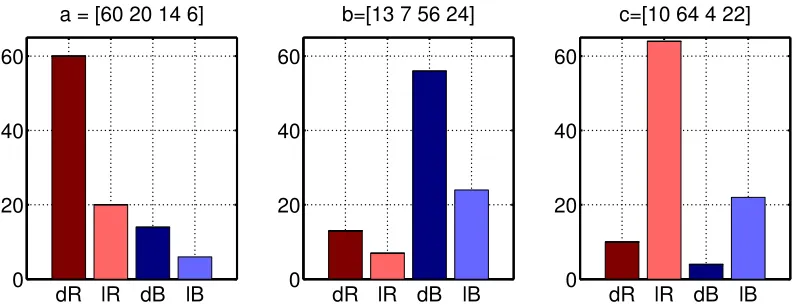
The fundamental idea behind optimal transport distances is that they can be used to com-pare histograms of features, when the features lie in a metric space and can therefore be compared one with the other. To illustrate this idea, suppose we wish to compare images of 10×10 = 100 pixels. Suppose further, for the sake of simplicity, that these pixels can only take values in a range of 4 possible colors,dark red,light red,dark blueandlight blue, and that each image is represented as a histogram of 4 colors as in Figure 1.
So called bin-to-bin distances (we provide a formal definition in Section 5.1) would compute the distance betweenaandbby comparing for each given indexitheir coordinates
ai and bi one at a time. For instance, computing the Manhattan distances (thel1 norm of
the difference of two vectors) of three histogramsa, bandc in Figure 1, we obtain thatais equidistant to b and c. However, upon closer inspection, assuming that dark and light red have more in common than, say, dark red and dark blue, one may have the intuition thatc
should be closer toathan it is tob. Optimal transport theory implements this intuition by carrying out an optimization procedure to compute a distance between histograms. Such an optimization procedure builds upon a set of feasible solutions (transport mappings) and a cost function (a linear cost), to define an optimal transport.
X =
13 7 56 24
10 4 40 6 60
1 1 11 7 20
1 2 4 7 14
1 0 1 4 6
(1)
dR lR dB lB 0
20 40 60
a = [60 20 14 6]
dR lR dB lB 0
20 40 60
b=[13 7 56 24]
dR lR dB lB 0
20 40 60
c=[10 64 4 22]
Figure 1: Three color histograms summing to 100. Althoughaand care arguably closer to each other because of their overlapping dominance in red colors, the Manhattan distance cannot consider such an overlap and treats all colors separately. As a result, in this example,ais equidistant from band c,ka−bk1 =ka−ck1 = 120.
possible color pairs, we obtain a 4×4 matrix which details, for each possible pair of colors (i, j), the overall amount xij of pixels of color iin awhich have been morphed into pixels
of color j inb. Because such a matrix representation only providesaggregated assignments and does not detail the actual individual assignments, such matrices are known as transport plans. A transport plan betweenaandbmust be such that its row and column sums match the quantities detailed in a and b, as highlighted on the top and right side of an example matrixX in Equation 1.
M =
• • • •
0 1 2 3 •
1 0 3 2 •
2 3 0 1 •
3 2 1 0 •
(2)
A Linear Cost for Transport Plans: A cost matrix M quantifies all 16 possible costs
mij of turning a pixel of a given color i into another color j. In the example provided in
Equation 3,M states for instance that the cost of turning a dark red pixel into a dark blue pixel is twice that of turning it into a light red pixel; that transferring a colored pixel from
a to the same color in b has a zero cost for all four colors. The cost of a transport plan
X, given the cost matrixM, is defined as the Frobenius dot-product ofX and M, namely hX, Mi=P
X?=
13 7 56 24
13 42 5 60
7 13 20
14 14
6 6
(3)
Smallest Possible Total Transport Cost: The transport distance is defined as the low-est cost one could possibly find by considering all possible transport plans from a to b. Computing such an optimum involves solving a linear program, as detailed in Section 2.3. For aand b and given M above, solving this program would return an optimal matrix X?
provided in Equation (3) with an optimum of hX?, Mi = 120. When comparing a and c, the distance would, on the other hand, be equal to 72. Comparing these two numbers, we can see that the transport distance agrees with our initial intuition thatais closer tocthan
b by taking into account a metric on features. We define rigorously the properties of both the cost matrixM and the set of transport plans in the next section.
2.2 The Ingredients of Discrete Optimal Transport
Optimal transport distances between histograms are computed through a mathematical program. The feasible set of that program is a polytope of matrices. Its objective is a linear function parameterized by metric matrices. We define both in the sections below.
2.2.1 Objective: Semimetric and Metric Matrices
Considerdpoints labeled as {1,2, . . . , d}in a metric space. Form now thed×dmatrixM
where element mij is equal to the distance between points i and j. Because of the metric
axioms, the elements ofM must obey three rules: (1) symmetry: mij =mji for all pairs of
indices i, j; (2) mii = 0 for all indicesi and more generallymij ≥0 for any pair (i, j); (3)
triangle inequality: mij ≤mik+mkj, for all triplets of indices i, j, k. The set of all d×d
matrices that observe such rules, and thus represent hypothetically the pairwise distances between dpoints taken in any arbitrary metric space, is known as the cone of semimetric matrices,
Mdef=nM ∈Rd×d: ∀1≤i, j, k ≤d, m
ii= 0, mij ≤mik+mkj
o
⊂Rd+×d.
Note that the d2symmetry conditionsmij =mjiand non-negativity conditionsmij ≥0 are
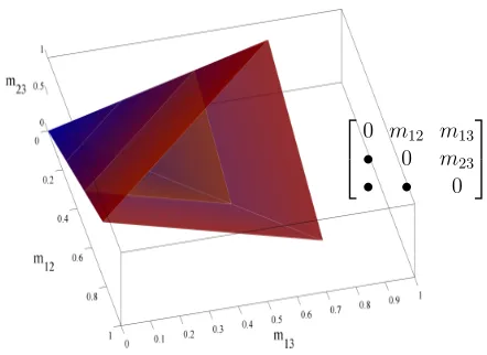
contained in thed3 linear inequalities described in the definition above. Mis a polyhedral set, because it is defined by a finite set of linear equalities and inequalities. M is also a convex pointed cone as can be visualized in Figure 2 ford= 3. Additionally, if a matrixM
satisfies conditions (1) and (3) but also has, in addition to (2), the property that mij >0
whenever i6=j, then we call M a metric matrix. We write M+⊂ M for the set of metric
matrices, which is neither open nor closed.
2.2.2 Feasible Set: Transport Polytopes
Consider two vectorsr andc in the simplex Σd. LetU(r, c) be the set ofd×dnonnegative
0 m12 m13 • 0 m23 • • 0
Figure 2: Semimetric cone in 3 dimensions. Ad×dmetric matrix ford= 3 can be described by 3 positive numbersm12, m13andm23that follow the three triangle inequalities, m12 ≤m13+m23, m13≤ m12+m23, m23 ≤m12+m13. The set (neither open nor closed) ofpositive triplets (m12, m13, m23) forms the set of metric matrices.
writing1d∈Rdfor the column vector of ones,
U(r, c) ={X∈Rd+×d|X1d=r, X>1d=c}.
Because of these constraints, it is easy to see that any matrixX= [xij] inU(r, c) is such that
P
ijxij = 1. Whilerandccan be interpreted as two probability measures on the discrete set
{1, . . . , d}, any matrixX inU(r, c) is thus a probability measure on{1, . . . , d} × {1, . . . , d}, the cartesian product of {1, . . . , d} with itself. U(r, c) can be identified with the set of all discrete probabilities on{1, . . . , d} × {1, . . . , d}that admitr and cas their first and second marginals respectively.
U(r, c) is a bounded polyhedron (the entries of any X in U(r, c) are bounded between 0 and 1) and is thus a polytope with a finite set of extreme points. This polytope has an effective dimension of d2 − 2d+ 1 in the general case where r and c have positive coordinates (Brualdi 2006, §8.1). U(r, c) is known in the operations research literature as the set of transport plans betweenr andc (Rachev and R¨uschendorf 1998). When r and c
are integer valued histograms with the same total sum, a transport plan with integral values is also known as a contingency table or a two-way table with fixed margins (Lauritzen 1982, Diaconis and Efron 1985).
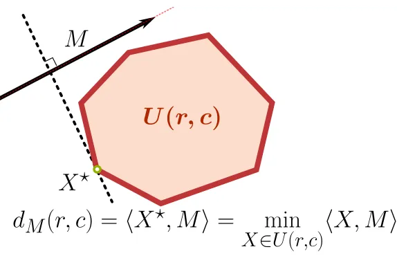
2.3 Optimal Transport Distances
Given two histogramsr andc of Σd and a matrix M, the quantity
G(r, c;M)def= min
X∈U(r,c)
M
d
M
(
r, c
) =
h
X
?
, M
i
=
min
X∈U
(
r,c
)
h
X, M
i
U
(
r, c
)
X
?
Figure 3: Schematic view of the optimal transport distance. Given a feasible set U(r, c) and a cost parameterM ∈ M+, the distance betweenr and cis the minimum of hX, Mi when X varies across U(r, c). The minimum is reached here at X?.
describes the optimum of a linear program whose feasible set is defined by r and c and whose cost is parameterized by M. G is a positive homogeneous function of M, that is
G(r, c;tM) = tG(r, c;M) for t≥0. G(r, c;M) can also be described as minus the support function (Rockafellar 1970,§13) of the polytopeU(r, c) evaluated at−M. A schematic view of that LP is given in Figure 3.
WhenM belongs to the cone of metric matricesM, the value ofG(r, c;M) is a distance (Villani 2003, §7, p.207) between r and c, parameterized by M. In that case, assuming implicitly thatM is fixed and onlyr andc vary, we will refer toG(r, c;M) as dM(r, c), the
optimal transport distance betweenr andc.
Theorem 1 dM is a distance on Σd whenever M ∈ M+.
The fact thatdM(r, c) is a distance is a well known result; a standard proof for continuous
probability densities is provided in Villani (2003, Theorem 7.3). A proof often reported in the literature for the discrete case can be found in Rubner et al. (2000). We believe this proof is not very clear, so we provide an alternative proof in the Appendix.
When r and c are, on the contrary, considered fixed, we will use the notation Grc(M)
to stress that M is the variable argument of G, as will be mostly the case in this paper. Although using two notations for the same mathematical object may seem cumbersome, these notations will allow us to stress alternatively which of the three variables r, cand M
are considered fixed in our analysis.
2.3.1 Extensions of Optimal Transport Distances
The distance dM bears many names: 1-Wasserstein; Monge-Kantorovich; Mallow’s
have also proposed to extend the optimal transport distance to compare unnormalized his-tograms, that is vectors with nonnegative coordinates which do not necessarily sum to 1. Simply put, these extensions compute a distance between two unnormalized histograms u
and v by combining any difference in the total mass ofu and v with the optimal transport plan that can carry the whole mass ofu onto v ifkuk1 ≤ kvk1 orv onto u ifkvk1 ≤ kuk1.
These extensions can also be traced back to earlier work by Kantorovich and Rubinshtein (1958), see Vershik (2006) for a historical perspective. We will not consider such extensions in this work, and will only consider distances for histograms of equal sum.
2.3.2 Relationship with Other Distances
The optimal transport distance bears an interesting relationship with the total variation distance, which is a popular distance between histograms of features in computer vision following early work by Swain and Ballard (1991). As noted by Villani (2003, p.7 & Ex.1.17 p.36), the total variation distance, defined as
dTV(r, c) def
= 1
2kr−ck1,
can be seen as a trivial instance of optimal transport distances by simply noting that
dTV=dM1,
where M1 is the matrix of ones with a zero diagonal, namely M1(i, j) is equal to 1 if
i = j and zero otherwise. The metric on features defined by M1 simply states that all
d considered features are equally different, that is their pairwise distances are constant. This relationship between total variation and optimal transport can be compared to the analogous observation that Euclidean distances are a trivial instance of the Mahalanobis family of distances, by setting the Mahalanobis parameter to the identity matrix. Tuning the ground metric M to select an optimal transport distance dM can thus be compared to
the idea of tuning a positive-definite matrix Ω to define a suitable Mahalanobis distance for a given problem: Mahalanobis distances are to the Euclidean distance what optimal transport distances are to the total variation distance, as schematized in Figure 4. We discuss this parallel further when reviewing related work in Section 5.2.
2.3.3 Computing Optimal Transport Distances
The distance dM between two histograms r and c can be computed as the solution of the
following Linear Program (LP),
dM(r, c) = minimize Pdi,j=1mijxij
subject to Pd
j=1xij =ri,1≤i≤d
Pd
i=1xij =cj,1≤j≤d xij ≥0,1≤i, j≤d.
This program is equivalent to the following program, provided in a more compact form, as:
dM(r, c) = minimize mTx
subject to Ax=
r c
∗
x≥0,
Figure 4: Contour plots of the Euclidean (top-left) and Total variation (bottom-left) of all points in the simplex ford= 3 to the point [0.5,0.3,0.2], and their respective pa-rameterized equivalents, the Mahalanobis distance (top-right) and the transport distance (bottom-right). The parameter for the Mahalanobis distance has been drawn randomly. The upper right values of the ground metricM are 0.8 and 0.4 on the first row and 0.6 on the second row.
whereAis the (2d−1)×d2 matrix that encodes the row-sum and column-sum constraints forX to be in U(r, c) as
A=
11×d⊗Id
Id⊗11×d
∗
,
where ⊗ is Kronecker’s product and the lower subscript ·
∗ in a matrix (resp. a vector) means that its last line (resp. element) has been removed. This modification is carried out to make sure that all constraints described by Aare independent, or equivalently that AT
2.4 Properties of the Optimal Transport Distance Seen As a Function of M
When both its arguments are fixed, the optimal transport distancedM(r, c) seen as a
func-tionGrcofM has three important properties: Grcis piecewise linear; concave; a subgradient
of Grccan be directly recovered by considering any optimal solution of the linear program
considered to compute Grc. These properties are crucial, because they highlight that for a
given pair of histograms (r, c), a gradient direction to increase or decreasedM(r, c) can be
obtained through the optimal transport plan that realizes dM(r, c), and that maximizing
this value is a convex problem.
2.4.1 Concavity and Piecewise-linearity
Because its feasible setU(r, c) is a bounded polytope and its objective is linear, Problem (4) has an optimal solution in the finite set Ex(r, c) of extreme points ofU(r, c) (Bertsimas and Tsitsiklis 1997, Theorem 2.7, p.65). Grcis thus the minimum of a finite collection of linear
functions, each indexed by an extreme point, and thus
Grc(M) = min
X∈U(r,c)hX, Mi=X∈minEx(r,c)hX, Mi, (5)
is piecewise linear. Grc is also concave by a standard result stating that the point-wise
minimum of a family of affine functions is itself concave (Boyd and Vandenberghe 2004, §3.2.3).
2.4.2 Differentiability
Because the computation of Grc involves a linear program, the gradient ∇Grc of Grc at a
given pointM is equal to the optimal solution X? to Problem (4) whenever this solution is unique,
∇Grc=X?,
as stated by Bertsimas and Tsitsiklis (1997, Theorem 5.3). Intuitively, by continuity of all functions involved in Problem (4) and the uniqueness of the optimal solution X?, one can show that there exists a ball with a positive radius around M for which Grc(M) is locally
linear, equal tohX?, Mi on that ball, resulting in the fact that the gradient ofhX?, Mi is
simply X?. More generally and regardless of the uniqueness of X?, any optimal solution
X? of Problem (4) is in the sub-differential∂Grc(M) of GrcatM (Bertsimas and Tsitsiklis
1997, Lemma 11.4). Indeed, suppose that Z(p) is the minimum of a linear program Z
parameterized by a cost vector x, over a bounded feasible polytope with extreme points {c1, . . . , cm}. Z(x) can in that case be written as
Z(x) = min
i=1,...,mui+c T i x.
Then, defining E(x) = {i|Z(x) = ui+cTi x}, namely the set of indices of extreme points
which are optimal for x, Bertsimas and Tsitsiklis (1997, Lemma 11.4) show that for any fixed x and any indexiinE(x), ci is a subgradient of Z at x. More generally, this lemma
also shows that the differential ofZ atxis exactly the convex hull of those optimal solutions {ci}i∈E(x). If, as in Equation (5), these ci’s describe the set of extreme points of U(r, c),
transport is necessarily in the subdifferential of Grc(M), and that this subdifferential is
exactly the convex hull of all the optimal transports betweenr and c using costM. In summary, the distancedM(r, c) seen as a function ofM (Grc(M) using our notations)
can be computed by solving a network flow problem, and any optimal solution of that network flow is a subgradient of the distance with respect to M. This function itself is concave in M. We use extensively these properties in Section 4 when we optimize the criteria considered in the next section.
3. Learning Ground Metrics as an Optimization Problem
We define in this section a family of criteria to quantify the relevance of a ground metric to compare histograms in a given learning task. We use to that effect a training sample of histograms with additional information.
3.1 Training Set: Histograms and Side Information
Suppose that we are given a sample{r1, . . . , rn} ⊂Σdof histograms in the canonical simplex
along with a family of coefficients {ωij}1≤i,j≤n, which quantify how similar ri and rj are.
We assume that these coefficients are such thatωij is positive wheneverri and rj describe
similar objects and negative for dissimilar objects. We further assume that this similarity is symmetric,ωij =ωji. The similarity of an object with itself will not be considered in the
following, so we simply assume thatωii= 0 for 1≤i≤n.
In the most simple case, these weights may reflect a labeling of all histograms into multiple classes and be set toωij >0 wheneverriandrj come from the same class andωij <
0 for two different classes. An ever simpler setting which we consider in our experiments is that of settingωij =1yi=yj, where the label yi of histogram ri for 1≤i≤n is taken in
a finite set of labels L ={1,2, . . . , L}. Let us introduce more notations before moving on to the next section. Since by symmetry ωij =ωji and Grirj =Grjri, we restrict the set of
pairs of indices (i, j) we will study to
Idef={(i, j)|i, j∈ {1, . . . , n}, i < j},
and introduce two subsets of I, the subsets of similar and dissimilar histograms:
E+def={(i, j)∈ I |ωij >0}; E−def={(i, j)∈ I |ωij <0}.
Finally, we define the shorthand Gij def
=Grirj.
3.2 Feasible Set of Metrics
We propose to formulate the ground metric learning problem as that of finding a metric matrix M ∈ M+ such that the corresponding optimal transport distance dM computed
between pairs of points in (r1, . . . , rn) agrees with the weightsω. However, because
constant to all its off-diagonal elements. Moreover, and as remarked earlier, two histograms
r and c define a homogeneous function Grc of M, that isGrc(tM) =t Grc(M). To remove
this ambiguity on the scale of M, we only consider in the following matrices that lie in the intersection ofM and the unit sphere inRd×dof the 1-norm,
M1 =M ∩B1,
whereB1 ={A∈Rd×d| kAk
1def=kak1 = 1}. M1 is convex as the intersection of two convex
sets. In what follows we call matrices in M1 metric matrices (this is a slight abuse of language since some of these matrices are in fact semimetrics).
3.3 A Local Criterion to Select the Ground Metric
More precisely, this criterion will favor metricsM for which the distancedM(ri, rj) issmall
for pairs ofsimilarhistogramsriandrj (ωij >0) andlargefor pairs ofdissimilarhistograms
(ωij <0). We build such a criterion by considering the family of all n2
pairs
{(ωij, Gij(M)),(i, j)∈ I}.
Given the ith datum of the training set, we consider the subsets Ei+ and Ei− of points that share their label withri and those that do not respectively:
Ei+def={j|(i, j) or (j, i)∈ E+}, Ei−def={j|(i, j) or (j, i)∈ E−}.
Within these subsets, we consider the setsNik+ and Nik−, which stand for the indices of any
k nearest neighbours of ri using distance dM and whose indices are taken respectively in
the subsetsEi+ andEi−. For each indexiand corresponding histogramri, we can now form
the weighted sum of distances to its similar and dissimilar neighbors
Sik+(M)def= X
j∈Nik+
ωijGij(M), and Sik−(M)def=
X
j∈Nik−
ωijGij(M). (6)
Note that Nik+ and Nik− are not necessarily uniquely defined. Whenever more than one list of indices can qualify as thekclosest neighbors of ri, we select such a list randomly among
all possible choices. We adopt the convention thatNik+=Ei+whenever kis larger than the
cardinality ofEi+, and follow the same convention forNik−. We use these two terms to form our final criterion:
Ck(M) def
=
n
X
i=1
Sik+(M) +Sik−(M). (7)
4. Approximate Minimization of Ck
Since all functionsGij are concave, Ck can be cast as a difference of convex functions Ck(M) =Sk−(M)− -Sk+(M),
where both
Sk−(M)def=
n
X
i=1
Sik−(M) and -Sk+(M)def=
n
X
i=1
are convex, by virtue of the convexity of each of the terms Sik− and -Sik+ defined in Equa-tion (6). This follows in turn from the concavity of each of the distances Gij as discussed
in Sections 2.4 and 3.3, and the fact that such functions are weighted by negative factors,
ωij for (i, j) ∈ E− and -ωij for (i, j) ∈ E+. We propose an algorithm to approximate the
minimization of Ck defined in Equation (7) that takes advantage of this decomposition.
4.1 Subdifferentiability of Ck
It is easy to see that, using the results onGrcwe have recalled in Section 2.4.1, the gradient
of Ck computed at a given metric matrixM is
∇Ck(M) =∇Sk−(M) +∇Sk+(M),
where,
∇Sk+(M) =
n
X
i=1
X
j∈Nik+
ωijXij?, ∇S
−
k(M) = n
X
i=1
X
j∈Nik−
ωijXij?,
whenever all solutions Xij? to the linear programs Gij considered in Ck are unique and
whenever each of the two sets ofk nearest neighbors of each histogram ri is unique. Also
as recalled in Section 2.4.1, any optimal solution Xij? is in the sub-differential ∂Gij(M) of Gij atM and we thus have that
n
X
i=1
X
j∈Nik+
ωijXij? ∈∂Sk+(M), n
X
i=1
X
j∈Nik−
ωijXij? ∈∂Sk−(M),
regardless of the unicity of the nearest-neighbors sets of each histogram ri. The details of
the computation ofSk−(M) and of the subgradient described above are given in Algorithm 1. The computations forSk+(M) are analogous to those ofS−k(M) and we use the abbreviation
Sk±(M) to consider either of these two cases in our algorithm outline.
4.2 Local Linearization of the Concave Part of Ck
We describe in Algorithm 2 a simple approach to obtain an approximate solution to the problem of minimizingCkwith a projected subgradient descent and a local linearization of
the concave part of Ck. Algorithm 2 runs a subgradient descent on Ck using two nested
loops: we linearize the concave part of Ck in an outer loop and minimize the resulting
convex approximation in the inner loop.
More precisely, the first loop is parameterized with an iteration counterp and starts by computing bothSk+(the concave part ofCk) and a vectorγ+ in its subdifferential using the
current candidate metric Mp. Using this value and the subgradient γ+, the concave part Sk+ of Ck can be locally approximated by its first order Taylor expansion,
Ck(M)≈S−k(M) +Sk+(Mp) +γ+T(M −Mp).
This approximation is convex, larger than Ck and can be minimized in an inner loop using
Algorithm 1Computation ofz=Sk±(M) and a subgradientγ, where±is either + or−.
Input: M ∈ M1.
for (i, j)∈ E± do
Compute the optimumz?ij and an optimal solutionXij? for Problem (4) with cost vector
mand constraint vector [ri;rj]∗. end for
Set G= 0, z = 0.
for i∈ {1,· · · , n}do
Select the smallestk elements ofz?ij, j∈ Ei± to define the set of neighborsNik±.
forj∈Nik± do G←G+ωijXij?. z←z+ωijz?. end for
end for
Output z and γ=g+g.
sufficient precision, we obtain a point
Mp+1∈argmin M∈M1
Sk−(M) +Sk+(Mp) +γT+(M−Mp).
We incrementpand repeat the linearization step described above. The algorithm terminates when sufficient progress in the outer loop has been realized, at which point the matrix computed in the last iteration is returned as the output of the algorithm.
The overall quality of the solution obtained through this procedure is directly linked to the quality of the initial point M0. The selection of M0 requires thus some attention. We provide a few options to selectM0 in the next section.
4.3 Initial Points
SinceCkis not a convex criterion, particular care needs to be taken to initialize our descent
algorithm. We propose in this section two approaches to choose the initial point M0.
4.3.1 The Total Variation Distance as an Optimal Transport Distance
The total variation distance between two histograms, defined as half the l1 norm of their
difference, can provide an educated guess to define an initial point M0 to optimize Ck.
Indeed, as explained in Section 2.3, the total variation distance can be interpreted as the optimal transport distance parameterized with the uniform ground metric M1 which is a matrix equal to 1 on all its off-diagonal terms and 0 on the diagonal. Therefore, we consider
M1(divided byd(d−1) to normalize it) in our experiments to initialize Algorithm 2. Since
Ckis not convex, usingM1is attractive from a numerical point of view becauseM1exhibits
the highest entropy among all matrices inM1. This choice has, however, two drawbacks:
• Because all the costs enumerated in M1 are equal, one can show that for a pair
Algorithm 2 Projected Subgradient Descent to minimizeCk Input M0∈ M1 (see Section 4.3), gradient stept0.
t←1.
p←0, M0out←M0.
while p < pmax or insufficient progress forzpout do
Use Algorithm 1 to computez+def=Sk+(Mpout) andγ+.
q←0, Min
0 ←Mpout.
whileq < qmax or insufficient progress for zqin do
Compute γ− andz− of Sk− using Algorithm 1 withMqin, (i, j)∈ E−.
Setzqin←z−+z++γ+T(minq −moutp ) .
SetMqin+1 ←PM1
minq − √t0
q(γ++γ−)
.
q ←q+ 1.
t←t+ 1.
end while Mout
p+1 ←Mqin. p←p+ 1.
end while Output Mout
p .
diagonal elements, namely any matrix X in the convex set {X∈U(r, c)|xii= min(ri, ci)}
is optimal. As a result, any matrix in that set is in the subdifferential ofGrc atM1.
Solvers that build upon the network simplex will return an arbitrary vertex within that set, mostly depending on the pivot rule they use. The very first subgradient descent iteration is thus likely to be extremely uninformative, and this should be reflected by a poor initial behaviour which we do indeed observe in practice.
• Because such a starting point ignores the information provided by all histograms {ri,1 ≤ i≤ n} and weights{ωij,(i, j) ∈ I}, we expect it to be far from the actual
optimum.
We propose an alternative approach in the next section: we approximate Ck by a linear
function of M and setM0 to be the minimizer of that approximation.
4.3.2 Linear Approximations to Ck and Independence Tables
We propose to form an initial point M0 by replacing the optimization underlying the
com-putation of each distance Gij(M) by a dot product, Gij(M) = min
X∈U(ri,rj)
hM, Xi ≈ hM,Ξiji,
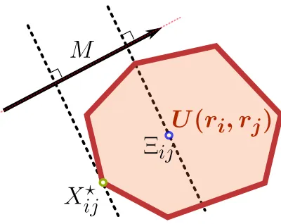
where Ξij is a representative matrix of the polytope U(ri, rj). This idea is illustrated in
have chosen such matrices, we replace now each term Gij in the criterion presented in
Equation (7) by the corresponding quantity hM,Ξiji and obtain an approximation χk of Ck parameterized by a matrix Ξk,
χk(M) def
=hM,Ξki, where Ξk def
=
n
X
i=1
X
j∈Nik−∪Nik+
ωijΞij,
where theknearest neighbors of each histogramri defined inNik−andNik+are those selected
by considering the total variation distance. To select a candidate matrixM that minimizes this criterion, we consider the following penalized problem,
min
M∈MλhM,Ξki+kMk
2
2= min M∈MkM+
λ
2Ξkk
2
2, λ >0, (8)
which can be solved using the approach described by Brickell et al. (2008, Algorithm 3.1). Brickell et al. propose triangle fixing algorithms to obtain projections on the cone of dis-tances under various norms, including the Euclidean distance. They study in particular the following problem,
min
M∈MkM−Hk2, (9)
where H is a symmetric nonnegative matrix that is zero on the diagonal. It is however straightforward to check that these three conditions, although intuitive when considering the metric nearness problem (Brickell et al. 2008,§2), are not necessary for Algorithm (3.1) described by Brickell et al. (2008, §3) to work. This algorithm is not only valid for non-symmetric matrices H as pointed out by the authors themselves, but it is also applicable to matrices H with negative entries and non-zero diagonal entries. Problem (8) can thus be solved by replacingH by −λ2Ξk in Problem (9) regardless of the sign of the entries of Ξ.
Note that other approaches could be considered to minimize the dot product hM,Ξi using alternative regularizers. Frangioni et al. (2005) propose for instance to handle lin-ear programs in the intersection between the cone of metrics and the set of polyhedral constraints{Mik+Mkj+Mij ≤2}which defines what is known as the metric polytope.
The techniques presented above build upon a linear approximation of each function
Gij(M) ashM,Ξiji by selecting a particular matrix Ξij such thatGij(M)≈ hM,Ξiji. We
propose to use a simple proxy for the optimal transport distance: the dot-product of M
with a matrix that lies at the center of U(r, c), as illustrated in Figure 5. We consider for such a center the independence table rcT (Good 1963). The table rcT, which is in U(r, c) becausercT1d=r and crT1d=c, is also the maximal entropy table inU(r, c), that is, the
table which maximizes
h(X) =−
d
X
p,q=1
XpqlogXpq.
Using the independence table to approximateGij, that is using the approximation
min
X∈U(ri,rj)
M
U
(
r
i
, r
j
)
X
ij
?
Ξ
ij
Figure 5: Schematic view of the approximation minX∈U(ri,rj)hM, Xi ≈ hM,Ξiji carried
out when using a central transport table Ξij instead of the optimal tableXij? to
compareri and rj.
provides us with a weighted center,
Ξk= n
X
i=1
X
j∈Nik−∪Nik+
ωijrirjT.
Note however that this approximation tends to overestimate substantially the distance between two similar histograms. Indeed, it is easy to check thatrTM r is positive whenever
r has positive entropy. In the case where all coordinates of r are equal to 1/d, rTM r is kMk1/d2. To close this section, one may notice that several methods can be used to compute centers for polytopes such asU(r, c), among which the Chebyshev center, the analytic center, or the center of the L¨owner-John ellipsoid, all described by Boyd and Vandenberghe (2004, §8.4,§8.5). We have not considered these approaches because computing them involve, unlike the independence table proposed above, the resolution of large convex programs or LP’s. Barvinok has, on the other hand, proposed recently a new center tailored specifically for transport polytopes, that he calls the typical table (2010). The typical table can be computed efficiently, both in theory and practice, as the result of a convex program of 2d
variables (Barvinok 2010, p.523). Experimental results indicate that they perform very similarly to independent tables so we do not explore them further in this paper.
In summary, we propose in this section to approximate Ck by a linear function and
compute its minimum in the intersection M1 of thel1 unit sphere and the cone of metric
matrices. This linear objective can be efficiently minimized using a set of tools proposed by Brickell et al. (2008) adapted to our problem. In order to propose such an approximation, we have used the independence tables as representative points of the polytopes U(ri, rj). The
Algorithm 3 Initial PointM0 to minimizeCk
Set Ξ = 0.
for i∈ {1,· · · , n}do
Compute the neighborhood setsNik+andNik−of histogramriusing an arbitrary distance,
for example, the total variation distance.
forj∈Nik+∪Nik− do
Ξ←Ξ +ωijrirjT. end for
end for
Set M0 ←minM∈MkM +λ2Ξk2 (Brickell et al. 2008, Algorithm 3.1). Output M0. optional: regularize M0 by setting M0←λM0+ (1−λ)M1.
5. Related Work
We provide in this section an overview of other distances for histograms of features. We start by presenting simple distances on histograms and follow by presenting metric learning approaches.
5.1 Metrics on the Probability Simplex
Deza and Deza (2009, §14) provide an exhaustive list of metrics for probability measures, most of which apply to probability measures on R and Rd. When narrowed down to dis-tances for probabilities on unordered discrete sets—the dominant case in machine learning applications—Rubner et al. (2000, §2) propose to split such distances into two families: bin-to-bin distances andcross-bin distances. Letr= (r1, . . . , rd)T and c= (c1, . . . , cd)T be
two histograms in the canonical simplex Σd.
Bin-to-bin distances only compare thedcouples of bin-counts (ri, ci)i=1..dindependently
to form a distance between r and c. The Jensen-divergence, χ2, Hellinger, total variation distances and more generally Csizarf-divergences (Amari and Nagaoka 2001,§3.2) all fall within this category. Notice that any of these divergences is known to work usually better for histograms than a straightforward application of the Euclidean distance as shown in our experiments or for instance by Chapelle et al. (1999, Table 4). This can be explained in theory using geometric (Amari and Nagaoka 2001, §3) or statistical arguments (Aitchison and Egozcue 2005).
Bin-to-bin distances are easy to compute and accurate enough to compare histograms when all dfeatures are sufficiently distinct. When, on the contrary, some of these features are known to be similar, either because of statistical co-occurrence (e.g., the words cat
and kitty) or through any other form of prior knowledge (e.g., pixel colors or amino-acid similarity) then a simple bin-to-bin comparison may not be accurate enough as argued by Rubner et al. (2000,§2.2). In particular, bin-to-bin distances are invariably large when they compare histograms with distinct supports, regardless of the fact that these two supports may in fact describe very similar features.
Cross-bin distances handle this issue by considering alld2 possible pairs (ri, cj) of
inRd is arguably the Mahalanobis family of distances,
dΩ(x, y) = q
(x−y)TΩ(x−y),
where Ω is a positive definited×dmatrix. The Mahalanobis distance betweenx andycan be interpreted as the Euclidean distance betweenLx and Ly whereL is a Cholesky factor of Ω or any square root of Ω. Learning such linear maps L or positive definite matrices Ω directly using labeled information has been the subject of a substantial amount of research in recent years. We briefly review this literature in the following section.
5.2 Mahalanobis Metric Learning
Xing et al. (2003), followed by Weinberger et al. (2006) and Davis et al. (2007) have proposed different algorithms to learn the parameters of a Mahalanobis distance. We refer to recent surveys by Kulis (2012) and Bellet et al. (2013) for more details on these approaches. These techniques define first a criterion and a feasible set of candidate matrices—either a positive semidefinite matrix Ω or a linear map L—to optimize the best parameter that fits best the data at hand. The criteria we propose in Section 3 are modeled along these ideas. Weinberger et al. (2006) were the first to consider criteria that only use nearest neighbors, which inspired in this work the proposal of Ck in Section 3.3.
We would like point out that Mahalanobis metric learning and ground metric learning have very little in common conceptually: Mahalanobis metric learning algorithms learn a
d×d positive semidefinite matrix or a m×d linear operator L. Ground metric learning learns instead ad×dmetric matrixM. The difference between Mahalanobis distances and optimal transport distances can be further highlighted by these simple identities:
dTV(r, c) =
1
2kr−ck1 =dM1(r, c), d2(r, c) =kr−ck2=d I(r, c)
The relationship between the Euclidean distance and the family of Mahalanobis distances, in which the former is a trivial instance of the latter when Ω is set to the identity matrix, is analogous to that between the total variation distance and optimal transport distances, in which the former is also a trivial instance of the latter where all distances between features are uniformly set to 1. The two families of distances evolve in related albeit completely different sets of distances, just like thel1 and l2 norms describe different geometries. An
il-lustration of this can be found in Figure 4 provided earlier in this paper, where the Euclidean and the total variation distances are compared with their parameterized counterparts. Both total variation and optimal transport distances havepiecewise linear level sets, whereas the Euclidean and Mahalanobis distances have ellipsoidal level sets.
5.3 Metric Learning in the Probability Simplex
Lebanon (2006) has proposed to learn a bin-to-bin distance in the probability simplex using a parametric family of distances parameterized by a histogram λ∈Σd−1 defined as
dλ(r, c) = arccos d
X
i=1
r
riλi rTλ
r
ciλi cTλ
!
.
This formula can be simplified by using the perturbation operator proposed by Aitchison (1986, p.46):
∀r, λ∈Σd−1, rλ def
= 1
rTλ(r1λ1,· · ·, rdλd) T.
Aitchison argues that the perturbation operation can be naturally interpreted as an addition operation in the simplex. Using this notation, the family of distancesdλ(r, c) proposed by
Lebanon can be seen as the standard Fisher metric applied to perturbed histogramsrλ
and cλ,
dλ(r, c) = arccosh
√
rλ,√cλi.
Using arguments related to the fact that a distance should vary according to the density of points described in a data set, Lebanon (2006) proposes to learn this perturbationλ in an unsupervised context, by only considering histograms but no other side-information.
More recently, Kedem et al. (2012) have proposed non-linear metric learning techniques, and focus more specifically on parameterizedχ2distances defined asdPχ2(r, c) =dχ2(P r, P c) where P can be any stochastic matrix P with unit row sums. We also note that, a few months after the publication on the arxiv of an early version of our paper, Wang and Guibas (2012) have proposed an algorithm that is very similar to ours, with the notable difference that they do not take into account metric constraints for the ground metric.
6. Experiments
We provide in this section a few details on the practical implementation of Algorithms 1, 2 and 3. We follow by presenting empirical evidence that ground metric learning improves upon other state-of-the-art metric learning techniques when considered on normalized his-tograms of low dimensions, albeit at a substantial computational cost.
6.1 Implementation Notes
6.2 Distances Used in this Benchmark
We consider five distances in this benchmark. Three classic bin-to-bin distances, Maha-lanobis distances with different learning schemes and the optimal transport distance cou-pled with ground metric learning. Bin-to-bin distances We consider thel1,l2 and Hellinger
distances on histograms,
l1(r, c) =kr−ck1, l2(r, c) =kr−ck2, H(r, c) =k
√
r−√ck2,
where√r is the vector whose coordinates are the squared roots of each coordinate ofr.
6.2.1 Mahalanobis Distances
We use the publicly available implementations of LMNN (Weinberger and Saul 2009) and ITML (Davis et al. 2007) to learn Mahalanobis distances for each task. We run both algorithms with default settings, that is k = 3 for LMNN and k = 4 for ITML. We use these algorithms on the Hellinger representations {√ri, i = 1, . . . , n} of all histograms
originally in the training set using the element-wise square root. We have considered this representation because the Euclidean distance between the Hellinger representations of two histograms corresponds exactly to the Hellinger distance (Amari and Nagaoka 2001, p.57). Since the Mahalanobis distance builds upon the Euclidean distance, we argue that this representation is more adequate to learn Mahalanobis metrics in the probability simplex. This observation is confirmed in all of our experimental results, where Mahalanobis metric learning approaches perform consistently better with the Hellinger transformation (see for instance the results reported in Figure 7).
6.2.2 Optimal Transport Distances with Ground Metric Learning
We learn ground metrics using the following settings. The neighborhood parameterkis set to 3 to be directly comparable to the default parameter setting of ITML and LMNN. In each classification task, and for two imagesri andrj, the corresponding weightωij is set to
1/nkif both histograms come from the same class and to−1/nkif they come from different classes. The subgradient stepsize t0 of Algorithm 2 is set to = 0.1, guided by preliminary
experiments and by the fact that, because of the normalization of the weightsωij, both the
current iterationMk in Algorithm 2 and subgradientsγ+ orγ−all have the same 1-norms. We carry out a minimum of 24 subgradient steps in each inner loop and set qmax to
80. Each inner loop is terminated when the objective does not progress more than 0.75% every 8 steps, or whenqreaches qmax. We carry out a maximum of 20 outer loop iterations.
6.3 Binary Classification
We study in this section the performance of ground metric learning when coupled with a nearest neighbor classifier on binary classification tasks generated with the Caltech-256 database.
6.3.1 Experimental Setting
We sample randomly 80 images for each of the 256 images classes2 of the Caltech-256 database. Each image is represented as a normalized histogram of GIST features (Oliva and Torralba 2001, Douze et al. 2009), obtained using an implementation provided by the INRIA-LEAR team.3 These features describe 8 edge directions at mid-resolution computed for each patch of a 4 ×4 grid on each image. Each feature histogram is of dimension
d= 8×4×4 = 128 and subsequently normalized to sum to one.
We select randomly 1,000 distinct pairs of classes among the 256 classes available in the data set to form as many binary classification tasks. For each pair, we split the 80 + 80 available points into 30 + 30 points to train distance parameters and 50 + 50 points to form a test set. This amounts to havingn= 60 training points following the notations introduced in Section 3.1. We consider in the following κ nearest neighbors approaches. Note that the neighborhood sizeκ and the parameter k used in metric learning approaches need not be the same. In our experiments κ varies, whereas k is always kept fixed, as detailed in Section 6.2.
6.3.2 Results
The most important results of this experimental section are summarized in Figure 6, which displays, for all considered distances, their average recall accuracy on the test set and the average classification error using a κ-nearest neighbor classifier. These quantities are averaged over 1,000 binary classifications. In this figure, GML paired with the the optimal transport distance dM is shown to provide, on average, the best performance with three
different metrics: the leftmost plot considers retrieval performance for test points and shows that, for each point considered on its own, GML-EMD selects on average more training points from the same class as closest neighbors than any other distance. The performance gap between GML-EMD and competing distances increases significantly as the number of retrieved neighbors is itself increased. The middle plot displays the average error over all 1,000 tasks of a κ-nearest neighbor classification algorithm when considered with all distances for varying values ofκ. The rightmost plot studies these errors in more detail for the case where the neighborhood parameter κ of nearest neighbors is 3. In this case too, GML combined with EMD fares significantly better than competing distances.
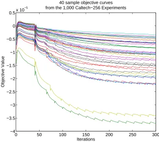
Figure 8 illustrates the empirical behavior of our descent algorithm. This plot displays 40 sample objective curves among the 1,000 computed to obtain the results above. The bumps that appear regularly on these curves correspond to the first update carried out after the linearization of the concave part of the objective. These results were obtained by setting the initial matrix toM1.
2. We do not consider theclutterclass in our experiments.
5 10 15 20 0.66
0.68 0.7 0.72 0.74 0.76 0.78
Number of retrieved Neighbours
Average Proportion of Correct Neighbours
Caltech−256 : Distance Accuracy on Test Data, Proportion of Correct Neighbors
L1 L2 Hellinger
LMNN k=3 (Hellinger) ITML k=4 (Hellinger) GML Ones k=3
1 3 5 7 9 11 13 15 17 19 0.18
0.2 0.22 0.24 0.26 0.28 0.3 0.32
Caltech−256 : κ−NN Test Error Averaged over 1,000 Binary Classifications
κ parameter in κ−NN
Classification Error Rate
0 0.1 0.2 0.3 0.4 0.5 0.6
L1 L2 Hellinger LMNN(H) ITML(H) GML Caltech−256: Distribution of 1,000 Classification Errors for κ=3
Data Set #Train #Test #Class Feature #Dim 20 News Group 600 19397 20 Topic Model (LDA) 100 Reuters 500 9926 10 Topic Model(LDA) 100
MIT Scene 800 800 8 SIFT 100
UIUC Scene 1500 1500 15 SIFT 100
OXFORD Flower 680 680 17 SIFT 100
CALTECH-101 3060 2995 102 SIFT 100
Table 1: Multiclass classification data sets and their parameters.
It is also worth mentioning as a side remark that the l2 distance does not perform as well as thel1or Hellinger distances on these data sets, which validates our earlier statement that the Euclidean geometry is usually a poor choice to compare histograms directly. This intuition is further validated in Figure 7, where Mahalanobis learning algorithms are shown to perform significantly better when they use the Hellinger representation of histograms.
Finally, Figure 9 describes the evolution of the average test error for two initial ground metrics, M1 and that which builds upon independence tables (Algorithm 3). Two conclu-sions can be drawn from this plot: First, independence tables provide on average a better initialization of the algorithm if only the first iterations of the algorithm are taken into account. However, this advantage seems to vanish as the number of subgradient descent iterations increases. Second, our algorithm does not seem to suffer from overfitting on av-erage, since the average error rate is a decreasing curve of the total number of iterations and does not seem to increase up to termination.
6.4 Multiclass Classification
We follow our experimental evaluation of ground metric learning by considering this time 6 multiclass classification data sets that consider text and image data.
6.4.1 Experimental Setting
The properties of the data sets and parameters used in our experiments are summarized in Table 1. The dimensions of the features have been kept low to ensure that the computation of optimal transports are tractable. We follow the recommended train/test splits for these data sets. If they are not provided, we split the data sets arbitrarily to form features using either LDA (Blei et al. 2003) or SIFT features (Lowe 1999). We then generate 5 random splits with the same balance to compute average accuracies over the entire data set.
6.4.2 Results
5 10 15 20 0.66
0.68 0.7 0.72 0.74 0.76 0.78
Number of retrieved Neighbours
Average Proportion of Correct Neighbours
Caltech−256 : Distance Accuracy on Test Data, Proportion of Correct Neighbors
L2 Hellinger LMNN k=3
LMNN k=3 (Hellinger) ITML k=4
ITML k=4 (Hellinger)
1 3 5 7 9 11 13 15 17 19 0.18
0.2 0.22 0.24 0.26 0.28 0.3 0.32
Caltech−256 : κ−NN Test Error Averaged over 1,000 Binary Classifications
κ parameter in κ−NN
Classification Error Rate
0 0.1 0.2 0.3 0.4 0.5 0.6
L2 Hellinger LMNN LMNN Hellinger ITML ITML Hellinger Caltech−256: Distribution of 1,000 Classification Errors for κ=3
Figure 7: The experimental setting in this figure is identical to that of Figure 6, except that only two different versions of LMNN and ITML are compared with the Hellinger and Euclidean distances. This figure supports our claim in Section 6.2.1 that Mahalanobis learning methods work better using the Hellinger representation of histograms,{√ri, i= 1, . . . , n}, rather than their straightforward representation
in the simplex{ri}i=1,...,n.
7. Conclusion and Future Work
0 50 100 150 200 250 300 −4
−3.5 −3 −2.5 −2 −1.5 −1 −0.5 0 0.5x 10
−5
40 sample objective curves from the 1,000 Caltech−256 Experiments
Iterations
Objective Value
Figure 8: 40 sample objective curves randomly selected among the 1,000 binary classifica-tion tasks run on the Caltech-256 data set. The initial point used here is the matrix M1 of ones and zero diagonal. The very first bumps usually observed
in the first iterations agree with our empirical findings on empirical test error displayed in Figure 9 which illustrate that the very first radients that are applied are usually not informative and result momentarily in an objective increase.
minimize approximately a criterion that is a difference of polyhedral convex functions. We propose two initial points to initialize this algorithm, and show that our approach provides, when compared to other competing distances, a superior average performance for a large set of image binary classification tasks using GIST features histograms, as well as different multiclass classification tasks. This improvement comes, however, with a heavy computational price tag.
1 3 5 7 9 11 13 15 17 19 0.18
0.19 0.2 0.21 0.22 0.23 0.24
κ parameter GML, M
0=1: Average Test Error
1 3 5 7 9 11 13 15 17 19
0.18 0.19 0.2 0.21 0.22 0.23 0.24
κ parameter GML, M
0=Ind: Average Test Error
5 Iterations 20 Iterations 50 Iterations 100 Iterations 150 Iterations Converged
0 50 100 150 200 Converged
0.19 0.2 0.21 0.22 0.23 0.24
3−NN Average Test Error as a function of Iteration Count
GML Ones k=3 GML Ind k=3
Figure 9: Average κ-nearest neighbor test error for GML using either the matrix of ones (top left) or the independent table (top right) described in Section 4.3. As can be seen forκ= 3 (bottom), initializing the algorithm withM1 performs worse than independence tables for a low iteration count. Yet this competitive advantage is reversed above a few iterations, as the algorithm converges. This figure also seems to indicate that, on average, the algorithm does not overfit the data since the average test error seems to decrease monotonically with the number of iterations, and becomes flat after 200 iterations. The experimental setting is identical to that of Figure 6.
5 10 15 0.15
0.2 0.25
20 News Group
Accuracy
5 10 15
0.4 0.45 0.5 0.55
Reuters
5 10 15
0.65 0.7 0.75
MIT Scene
Accuracy
5 10 15
0.45 0.5 0.55 0.6
UIUC Scene
5 10 15
0.2 0.25 0.3
OXFORD Flower
Neighborhood Size
Accuracy
5 10 15
0.15 0.2 0.25 0.3
CALTECH−101
Neighborhood Size GML
LMNN
LMNN−HELLINGER L1
L2 HELLINGER
Figure 10: κ-nearest neighbor performance for different distances on multi-class problems. Performance is averaged over 5 repeats, whose variability is illustrated with er-ror bars. Erer-rors are reported over varyingκ nearest neighbor parameters. Our benchmark considers three classical distances, l1, l2 and Hellinger, and their respective learned counterparts: GML paired with the transport distance ini-tialized with the matrixM1, classic LMNN and LMNN on the Hellinger repre-sentation.
problems which are provably faster to compute. Our work in this paper suggests on the other hand that the content (and not the structure) of the ground metric can be learned to improve classification accuracy. We believe that the combination of these two viewpoints could result in optimal transport distances that are both adapted to the task at hand and fast to compute. A strategy to achieve both goals would be to enforce such structural constraints on candidate metricsM when looking for minimizers of criteriaCk. We also believe that the
Acknowledgments
The authors would like to thank anonymous reviewers and the editor for stimulating com-ments. MC would like to thank Zaid Harchaoui and Alexandre d’Aspremont for fruitful discussions, as well as Tam Le for his help in preparing some of the experiments.
Appendix A.
Proof (Theorem 1) Symmetry and definiteness of the distance are easy to prove: since
M has a null diagonal, dM(x, x) = 0, with corresponding optimal transport matrix X? =
diag(x); by the positivity of all off-diagonal elements of M, dM(x, y) >0 whenever x6=y;
by symmetry of M, dM is itself a symmetric function in its two arguments. To prove the
triangle inequality, Villani (2003, Theorem 7.3) uses the gluing lemma. We provide here a self-contained version of this proof which provides an explicit formulation for the gluing lemma in the discrete case. Letx, y, z ∈Σd. Let P and Q be two optimal solutions of the
transport problems betweenxandy, andyandzrespectively. LetSbe thed×d×dtensor whose coefficients are defined as
sijk def
= pijqjk
yj ,
for all indices j such that yj >0. For indices j such thatyj = 0, the corresponding values sijk are set to 0. S is a probability measure on {1, . . . , d}3, as a direct consequence of the
fact that thed×dmatrixSi·k def
= [P
jsijk]ik is a transport matrix betweenx andzand thus
sums to 1. Indeed,
X
i
X
j
sijk=
X
j
X
i
pijqjk yj =X j qjk yj X i pij =
X
j qjk
yj yj =
X
j
qjk =zk (column sums) ,
X
k
X
j
sijk=
X
j
X
k
pijqjk yj =X j pij yj X k qjk =
X
j pij
yj yj =
X
j
pij =xi (row sums).
To obtain the triangle inequality, notice that Si·k being a matrix of U(x, z) we can write: dM(x, z) = min
X∈U(x,z)
hX, Mi ≤ hSi·k, Mi=
X
ik mik
X
j
pijqjk yj
≤X
ijk
(mij+mjk) pijqjk
yj
=X
ijk mij
pijqjk yj
+mjk pijqjk
yj
=X
ij
mijpij
X k qjk yj +X jk
mjkqjk
X i pij yj =X ij
mijpij+
X
jk
mjkqjk =dM(x, y) +dM(y, z),
References
R. Ahuja, T. Magnanti, and J. Orlin.Network Flows: Theory, Algorithms and Applications. Prentice Hall, 1993.
J. Aitchison. The Statistical Analysis of Compositional Data. Chapman & Hall, 1986.
J. Aitchison and J. Egozcue. Compositional data analysis: Where are we and where should we be heading? Mathematical Geology, 37(7):829–850, 2005.
S.-I. Amari and H. Nagaoka. Methods of Information Geometry. AMS vol. 191, 2001.
K. Ba, H. Nguyen, H. Nguyen, and R. Rubinfeld. Sublinear time algorithms for earth movers distance. Theory of Computing Systems, 48(2):428–442, 2011.
A. Barvinok. What does a random contingency table look like? Combinatorics, Probability and Computing, 19(04):517–539, 2010.
A. Bellet, A. Habrard, and M. Sebban. A survey on metric learning for feature vectors and structured data. arXiv:1306.6709, 2013.
D. Bertsimas and J. Tsitsiklis.Introduction to Linear Optimization. Athena Scientific, 1997.
D. Blei and J. Lafferty. Topic models. Text Mining: Classification, Clustering, and Appli-cations, 10:71, 2009.
D. Blei, A. Ng, and M. Jordan. Latent Dirichlet allocation. The Journal of Machine Learning Research, 3:993–1022, 2003.
S. Boyd and L. Vandenberghe. Convex Optimization. Cambridge University Press, 2004.
J. Brickell, I. Dhillon, S. Sra, and J. Tropp. The metric nearness problem. SIAM Journal of Matrix Analysis and Applications, 30(1):375–396, 2008.
R. A. Brualdi. Combinatorial Matrix Classes, volume 108. Cambridge University Press, 2006.
O. Chapelle, P. Haffner, and V. Vapnik. SVMs for histogram based image classification. IEEE Transactions on Neural Networks, 10(5):1055, Sept. 1999.
M. Cuturi. Sinkhorn distances: Lightspeed computation of optimal transport. InAdvances in Neural Information Processing Systems 26, pages 2292–2300. 2013.
J. Davis, B. Kulis, P. Jain, S. Sra, and I. Dhillon. Information-theoretic metric learning. In Proceedings of the 24th International Conference on Machine Learning, pages 209–216. ACM, 2007.
M. Deza and E. Deza. Encyclopedia of Distances. Springer Verlag, 2009.
M. Douze, H. J´egou, H. Sandhawalia, L. Amsaleg, and C. Schmid. Evaluation of GIST de-scriptors for web-scale image search. InProceedings of the ACM International Conference on Image and Video Retrieval. Article 19, ACM, 2009.
L. Ford and Fulkerson. Flows in Networks. Princeton University Press, 1962.
A. Frangioni, A. Lodi, and G. Rinaldi. New approaches for optimizing over the semimetric polytope. Mathematical Programming, 104(2):375–388, 2005.
I. Good. Maximum entropy for hypothesis formulation, especially for multidimensional contingency tables. The Annals of Mathematical Statistics, pages 911–934, 1963.
J. Gudmundsson, O. Klein, C. Knauer, and M. Smid. Small manhattan networks and algo-rithmic applications for the earth movers distance. In Proceedings of the 23rd European Workshop on Computational Geometry, pages 174–177, 2007.
T. Joachims. Learning to Classify Text Using Support Vector Machines: Methods, Theory, and Algorithms. Kluwer Academic Publishers, 2002.
L. Kantorovich and G. Rubinshtein. On a space of totally additive functions. Vestn Lening. Univ., 13:52–59, 1958.
H. Kashima, K. Tsuda, and A. Inokuchi. Marginalized kernels between labeled graphs. In Proceedings of the 20th International Conference on Machine Learning, pages 321–328, 2003.
D. Kedem, S. Tyree, K. Weinberger, F. Sha, and G. Lanckriet. Non-linear metric learning. In Advances in Neural Information Processing Systems 25, pages 2582–2590, 2012.
B. Kulis. Metric learning: A survey. Foundations & Trends in Machine Learning, 5(4): 287–364, 2012.
S. Lauritzen. Lectures on Contingency Tables. Aalborg Univ. Press, 1982.
G. Lebanon. Metric learning for text documents. IEEE Transactions on Pattern Analysis and Machine Intelligence, 28(4):497–508, 2006.
C. Leslie, E. Eskin, and W. S. Noble. The spectrum kernel: a string kernel for svm protein classific ation. In Proceedings of the Pacific Symposium on Biology 2002, pages 564–575, 2002.
E. Levina and P. Bickel. The earth mover’s distance is the Mallows distance: some insights from statistics. InProceedings of the Eighth IEEE International Conference on Computer Vision, volume 2, pages 251–256. IEEE, 2001.
D. Lowe. Object recognition from local scale-invariant features. InComputer Vision, 1999. The Proceedings of the Seventh IEEE International Conference on, volume 2, pages 1150 –1157 vol.2, 1999.
C. Mallows. A note on asymptotic joint normality. The Annals of Mathematical Statistics, pages 508–515, 1972.
A. Oliva and A. Torralba. Modeling the shape of the scene: A holistic representation of the spatial envelope. International Journal of Computer Vision, 42(3):145–175, 2001.
O. Pele and M. Werman. Fast and robust earth mover’s distances. In Proceedings of the International Conference on Computer Vision’09, 2009.
S. Rachev. Probability Metrics and the Stability of Stochastic Models. Wiley series in probability and mathematical statistics: Applied probability and statistics. Wiley, 1991.
S. Rachev and L. R¨uschendorf. Mass Transportation Problems: Theory, volume 1. Springer Verlag, 1998.
T. Rockafellar. Convex Analysis. Princeton University Press, 1970.
Y. Rubner, L. Guibas, and C. Tomasi. The earth movers distance, multi-dimensional scal-ing, and color-based image retrieval. In Proceedings of the ARPA Image Understanding Workshop, pages 661–668, 1997.
Y. Rubner, C. Tomasi, and L. Guibas. The earth mover’s distance as a metric for image retrieval. International Journal of Computer Vision, 40, 2000.
M. Swain and D. Ballard. Color indexing. International Journal of Computer Vision, 7(1): 11–32, 1991.
A. Vershik. Kantorovich metric: initial history and little-known applications. Journal of Mathematical Sciences, 133(4):1410–1417, 2006.
C. Villani. Topics in Optimal Transportation, volume 58. AMS Graduate Studies in Math-ematics, 2003.
F. Wang and L. J. Guibas. Supervised earth movers distance learning and its computer vision applications. In Computer Vision–ECCV 2012, pages 442–455. Springer, 2012.
K. Weinberger and L. Saul. Distance metric learning for large margin nearest neighbor classification. The Journal of Machine Learning Research, 10:207–244, 2009.
K. Weinberger, J. Blitzer, and L. Saul. Distance metric learning for large margin nearest neighbor classification. InAdvances in Neural Information Processing Systems 18, pages 1473–1480, 2006.
![Figure 4: Contour plots of the Euclidean (top-left) and Total variation (bottom-left) of allpoints in the simplex for d = 3 to the point [0.5, 0.3, 0.2], and their respective pa-rameterized equivalents, the Mahalanobis distance (top-right) and the transpor](https://thumb-us.123doks.com/thumbv2/123dok_us/9805980.1966535/9.612.163.448.87.391/euclidean-variation-allpoints-respective-rameterized-equivalents-mahalanobis-transpor.webp)