Fast Cross-Validation via Sequential Testing
Tammo Krueger [email protected]
Danny Panknin [email protected]
Mikio Braun [email protected]
Technische Universit¨at Berlin Machine Learning Group Marchstr. 23, MAR 4-1 10587 Berlin, Germany
Editor:Charles Elkan
Abstract
With the increasing size of today’s data sets, finding the right parameter configuration in model selection via cross-validation can be an extremely time-consuming task. In this pa-per we propose an improved cross-validation procedure which uses nonparametric testing coupled with sequential analysis to determine the best parameter set on linearly increas-ing subsets of the data. By eliminatincreas-ing underperformincreas-ing candidates quickly and keepincreas-ing promising candidates as long as possible, the method speeds up the computation while preserving the power of the full cross-validation. Theoretical considerations underline the statistical power of our procedure. The experimental evaluation shows that our method reduces the computation time by a factor of up to 120 compared to a full cross-validation with a negligible impact on the accuracy.
Keywords: cross-validation, statistical testing, nonparametric methods
1. Introduction
Model selection by cross-validation is a de-facto standard in applied machine learning to tune parameter configurations of machine learning methods in supervised learning settings (see Mosteller and Tukey 1968; Stone 1974; Geisser 1975 and also Arlot et al. 2010 for a recent and extensive review of the method). Part of the data is held back and used as a test set to get a less biased estimate of the true generalization error. Cross-validation is computationally quite demanding, though. Doing a full grid search on all possible combi-nations of parameter candidates quickly takes a lot of time, even if one exploits the obvious potential for parallelization.
cannot reflect the true complexity of the learning problem, the configurations selected by cross-validation will lead to underfitted models. On the other hand, a too large subset will take longer for the cross-validation to finish.
Effective use of model selection heuristics requires both an experienced practitioner and familiarity with the data set. However, as we will discuss in more depth below, the effect of taking subsets on the estimated generalization error is more manageable: Given increasing subsets of the data, the test errors converge to the values on the full data set for each parameter configuration, but the parameter configuration achieving the minimum test error will converge much faster. Thus, using subsets in a systematic way opens up a promising way to speed up the model selection process, since training models on smaller subsets of the data is much more time-efficient. During this process care has to be taken when an increase in available data suddenly reveals more structure in the data, leading to a change of the optimal parameter configuration. Still, as we will discuss in more depth, there are ways to guard against such change points, making the heuristic of taking subsets a more promising candidate for an automated procedure.
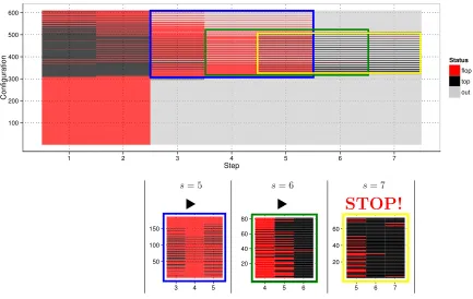
In this paper we will propose a method which speeds up cross-validation by considering subsets of increasing size. By removing clearly underperforming parameter configurations on the way this leads to a substantial saving in total computation time as sketched in Figure 1. In order to account for possible change points, sequential testing (Wald, 1947) is adapted to control asafety zone, roughly speaking, a certain number of allowed failures for a parameter configuration; at the same time this framework allows for dropping clearly underperforming configurations. Finally, we add a stopping criterion to watch for early convergence of the process to further speed up the computation. The resulting method thus consumes less time and space than a full grid cross-validation procedure at no significant loss in accuracy. We prove certain theoretical properties about its optimality, yet, this procedure relies on the availability of a vast amount of data to guide the decision process into a stable region where each configuration sees enough data to show its real performance.
In the following, we will first discuss the effects of taking subsets on learners and cross-validation (Section 2), discuss related work in Section 3, present our method Fast Cross-Validation via Sequential Testing (CVST, Section 4), state the theoretical properties of the method (Section 5) and finally evaluate our method on synthetic and real-world data sets in Section 6. Section 7 gives an overview of possible extensions and Section 8 concludes the paper. The impatient practitioner may skip some theoretical treatments and focus on the self-contained Section 4 describing the CVST algorithm and its evaluation in Section 6. To ease the reading process we collected our notational conventions in Table 1.
2. Cross-Validation on Subsets
Our approach is based on taking subsets of the data to speed up cross-validation. For this approach to work well, we need that the minima of the test errors give reliable estimates of the true performance already for small subsets. In this section, we will discuss the setting and motivate our approach. The goal is to understand which effects lead to making the estimates reliable.
Let us first introduce some notation: Assume that our N training data points di are
5-fold CV CVST 0.1 0.2 0.3 0.4 0.1 0.2 0.3 0.4 0.1 0.2 0.3 0.4 0.1 0.2 0.3 0.4 0.1 0.2 0.3 0.4 ●●●●●●●●●●●●●●●●●● ●●●●●● ●●●●●●● ●●●●●●●●●●●●●●●●●●●●●●●●●● ● ●●● ●●●●●●●●●●●●●●●●●● ●●●●●● ●●●●●●● ●●●●●●●●●●●●●●●●●●●●●●●●●● ● ●●● ●●●●●●●●●●●●●●●●●●●●● ●●●●●● ●●●●●●●●●●●●●●●●●●●●●●●●●●●●●● ● ●●● ●●●●●●●●●●●●●●●●●● ●●●●●● ●●●●●●● ●●●●●●●●●●●●●●●●●●●●●●●●●● ● ●●● ●●●●●●●●●●●●●●●●●● ●●● ●●●●●● ●●●●●●●●●●●●●●●●●● ●●●●●●●●●●●● ● ●●● fold 1 fold 2 fold 3 fold 4 fold 5
−4 −3 −2 −1 0 1 2 log(σ)
Class . Error 0.1 ● ●●●●●●●●●●●●●●●●●●●●●●●●●●●●●●●●●●● ● ● ● ● ● ● ● ● ● ● ● ● ● ● ● ● ● ● ● ● ● ● ● ● ● ● ● ● ● ● ● ● ● ● ● ● ● ● ● ● ● ● ● ● ● ● ● ● ● ● ● ● ● ● ● ● ● ● ● ● ● ● ● ● ● ● ● ● ● ● ● ● ● ● ● ● ● ● ● ● ● ● ● ● ● ● ● ● ● ● ● ● ● ● ● ● ● ● ● ● ● ● ● ● ● ● ● ● ● ● ● ● ● ● ● ● ● ● ● ● ● ● ● ● ● ● ● ● ● ● ● ● ● ● ● ● ● ● ● ● ● ● ● ● ● ● ● ● ● ● ● ● ● ● ● ● ● ● ● ● ● ● ● ● ● ● ● ● ● ● ● ● ● ● ● ● ● ● ● ● ● ● ● ● ● ● ● ● ● ● ● ● ● ● ● ● ● ● ● ● ● ● ● ● ● ● ● ● ● ● ● ● ● ● ● ● ● ● ● ● ● ● ● ● ● ● ● ● ● ● ● ● ● ● ● ● ● ● ● ● ● ● ● ● ● ● ● ● ● ● ● ● ● ● ● ● ● ● ● ● ● ● ● ● ● ● ● ● ● ● ● ● ● ● ● ● ● ● ● ● ● ● ● ● ● ● ● ● ● ● ● ● ● ● ● ● ● ● ● ● ● ● ● ● ● ● ● ● ● ● ● ● ● ● ● ● ● ● ● ● ● ● ● ● ● ● ● ● ● ● ● ● ● ● ● ● ● ● ● ● ● ● ● ● ● ● ● ●●● ● ●●●
−4 −3 −2 −1 0 1 2 log(σ)
Class . Error Size ● ● ● ● ● ● ● ● ● ● 100 200 300 400 500 600 700 800 900 1000 0 100 200 300 400 500 600
Cumulative Model Training Time
Configur ation 0 100 200 300 400 500 600
Cumulative Model Training Time
Configur ation Size 100 200 300 400 500 600 700 800 900 1000
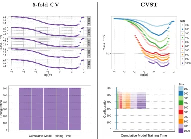
Figure 1: Performance of a 5-fold cross-validation (CV, left) and fast cross-validation via sequential testing (CVST, right): While the CV has to calculate the model for each configuration (here: σ of a Gaussian kernel) on the full data set, the CVST algorithm uses increasing subsets of the data and drops significantly underper-forming configurations in each step (upper panels), resulting in a drastic decrease of total calculation time (sum of colored area in lower panels).
distributionP onX × Y. We assume an example-wise loss function `:Y × Y →Rso that
the overall error or expected risk of a predictorg:X → Y is given byR(g) =E[`(g(X), Y)] where (X, Y)∼P. For some finite set of possible parameter configurations C, let gn(c) be
the predictor learned for parameter c∈C from the first ntraining examples.
The core procedure in a cross-validation approach is to train predictors for each c and consider their test error. Denote by gn(c) the predictor obtained by training on the firstn
points of the training data for parameterc. We wish to study whether this error converges asngrows. Let us denote by c∗n a configuration optimal for subset sizen:
R(gn(c∗n)) = min
c∈CR(gn(c)).
Symbol Description
di = (Xi, Yi)∈ X × Y Data points
N Total data set size
g:X 7→ Y Learned predictor
`:Y × Y 7→R Loss function
R(g) =E[`(g(X), Y)] Risk of predictor g
c Configuration of learner
C Finite set of examined configurations
gn(c) :X 7→ Y Predictor learned onndata points for configuration c
c∗ Overall best configuration
c∗n Best configuration for models based on ndata points
s Current step of CVST procedure
S Total number of steps
∆ =N/S Increment of model size
Pp Pointwise performance matrix
PS Overall performance matrix of dimension|C| ×S
TS Trace matrix of dimension|C| ×S
wstop Size of early stopping window
α, αl, βl Significance levels
π Success probability of a binomial variable
Table 1: List of symbols
In cross-validation, the true test error is not known and estimated by the empirical error on an independent test set. For the sake of simplicity, we will consider the true test error nevertheless for the remainder of this section. In our experience, the effects discussed below also hold for cross-validation, because the estimation error is small and does not create a systematic distortion of the choice of configuration.
Since we want to infer the performance of the predictor on the full training set based on its performance on a subset, we need that the errors are similar for a fixed configuration c
as the size of the subset approaches the full training set size. A necessary condition for this to hold in general is thatR(gn(c)) converges as n tends to infinity. Luckily, this holds for
most existing learning methods (see Appendix A for some examples). A counter example is the case ofk-nearest neighbor with fixedk. Training with k= 10 leads to quite different predictions on data sets of size 100 compared to, say, 10,000. More discussion can be found below in Section 5.3.
We are interested in the difference in errors between the best parameter configuration learned on the subset of sizen, and on the full data setN, that is, R(gn(cn∗))−R(gN(c∗N)).
This error can be bounded by considering the difference between R(gn(c)) and R(gN(c))
0.00 0.05 0.10
−4 −3 −2 −1 0 1 2
log(σ)
Size
10 25 50 75 100 150 200 250 300 350 400 450 500
(a)
0.00 0.05 0.10
−4 −3 −2 −1 0 1 2
lo g(σ)
c =
Size
10 100 500
estimation error
approximation error
R(gn(c))
(b)
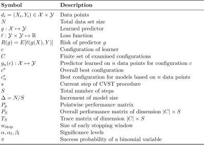
Figure 2: Test error of an SVR model on thenoisy sinc data set introduced in Section 6.1. We can observe a shift of the optimalσof the Gaussian kernel to the fine-grained structure of the problem, if we have seen enough data. In Figure (b), approxi-mation error is indicated by the black solid line, and the estiapproxi-mation error by the black dashed line. The minimal risk is shown as the blue dashed line. One can see that uniform approximation of the estimation error is not the main driving force, instead, the decay of the approximation error with smaller kernel widths together with an increase of the estimation error at small kernel widths makes sure that the minimum converges quickly.
which correspond to complex models, gn(c) may continue to improve right up to the full
number N of data points.
So while uniform convergence seems a sufficient condition, let us look at a concrete example to see whether uniform convergence is a necessary condition for convergence of the minima. Figure 2(a) shows the test errors for a typical example. We train a support vector regression model (SVR) on subsets of the full training set consisting of 500 data points. The data set is the noisy sinc data set introduced in Section 6.1. Model parameters are the kernel width σ of the Gaussian kernel used and the regularization parameter, where the results shown are already optimized over the regularization parameter for the sake of simplicity.
We see that the minimum converges rather quickly, first to the plateau of log(σ) ∈
[−1.5,−0.3] approximately, and then towards the lower one at [−2.5,−1.7], which is also the optimal one at training set size n = 500. We see that uniform convergence is not the main driving force. In fact, the errors for small kernel widths are still very far apart even when the minimum is already converged.
Section 2.4.3 in Mohri et al. 2012):
R(gn∗)−R∗ =
R(gn∗)−inf
g∈GR(g)
| {z }
estimation error
+
inf
g∈GR(g)−R ∗
)
| {z }
approximation error
.
The estimation error measures how far the chosen model is from the one which would be asymptotically optimal, while the approximation error measures the difference in risk between the best possible model in the hypothesis class and the true function.
Using this decomposition, we can interpret the figure as follows (see Figure 2(b)): The kernel width controls the approximation error. For log(σ)≥ −1.8, the resulting hypothesis class is too coarse to represent the function under consideration. It becomes smaller until it reaches the level of the Bayes risk as indicated by the dashed blue line. For even larger training set sizes, we can assume that it will stay on this level even for smaller kernel sizes. The difference between the blue line and the upper lines shows the estimation error. The estimation error has been extensively studied in statistical learning theory and is known to be linked to different notions of complexity like VC-dimension (Vapnik, 1998), fat-shattering dimension (Bartlett et al., 1996), or the norm in the reproducing kernel Hilbert space (RKHS) (Evgeniou and Pontil, 1999). A typical result shows that the estimation error can be bounded by terms of the form
R(g∗n)−inf
g∈GR(g)≤O
r
d(G) logn n
!
,
whered(G) is some notion of complexity of the underlying hypothesis class, and the bound holds with high probability. For our figure, this means that we can expect the estimation error to become larger for smaller kernel widths.
If we image the parameter configurations ordered according to their complexity, we see that for parameter configurations with small complexity (that is, large kernel width), the approximation error will be high, but the estimation error will be small. At the same time, for parameter configurations with high complexity, the approximation error will be small, even optimal, but the estimation error will be large, although it will decay with increasing training set size. In combination, the estimates at smaller training set sizes tend to underestimate the true model complexity, but as the estimation error decreases and becomes small compared to the approximation error, the minimum also converges to the true one. The fact that the estimation error is larger for more complex models acts as a guard to choose too complex models. The estimation error for models which have higher complexity than the optimal one can effectively be ignored. Therefore, we can expect much faster convergence than given by a uniform error bound, which is, however, highly data dependent.
enough to the true errors. A more formal study of the effects discussed above is therefore the subject of future work.
On the other hand, the mechanisms which lead to fast convergence of the minimum are plausible when looking at concrete examples as we did above. Therefore, we will assume in the following that the location of the best parameter configuration might initially change but then become more or less stable quickly. Note that we do not claim that the speed of this convergence is known. Instead, we will use sequential testing to introduce asafety zone
which will be as large as possible to ensure that our method is robust against these initial changes and good configurations survive till final stable regime.
3. Related Work
Using statistical tests and the sequential analysis framework in order to speed up learning has been the topic of several lines of research. However, the existing body of work mostly focuses on reducing the number of test evaluations, while we focus on the overall process of eliminating candidates themselves. To the best of our knowledge, this is a new concept and can apparently be combined with the already available racing techniques to further reduce the total calculation time.
Maron and Moore (1994, 1997) introduce the so-calledHoeffding Races which are based on the nonparametric Hoeffding bound for the mean of the test error. At each step of the algorithm a new test point is evaluated by all remaining models and the confidence intervals of the test errors are updated accordingly. Models whose confidence interval of the test error lies outside of at least one interval of a better performing model are dropped. In a similar vein Zheng and Bilenko (2013) have applied this concept to cross-validation and improve this approach by using paired t-test and power analysis to control both the false positive and false negative rate. Chien et al. (1995, 1999) devise a similar range of algorithms using concepts of PAC learning and game theory: Different hypotheses are ordered by their expected utility according to the test data the algorithm has seen so far. As for Hoeffding Races, the emphasis in this approach lies on reducing the number of evaluations. Thus, the application domain for these kind of algorithms is best suited where the evaluation of a data point given a learned model is costly. Since this approach expects that a model is fully trained before its evaluation, the direct utilization of racing algorithms for model selection would result in a procedure similar to a one-fold cross-validation: First learn a model on one half of the data and do the time efficient evaluation as described above on the other half. Obviously, this would yield a maximal relative time improvement of k compared to standard k-fold cross-validation since we learn one model instead of thek fork-fold cross-validation. Yet, the orthogonality of this approach to the CVST procedure could be utilized in each step and for each remaining configuration to further increase the runtime benefits by minimizing the necessary evaluations of a model for determining whether it belongs to the top configurations or not.
configu-rations. While Bradley and Schapire (2008) use similar concepts in the context of boosting (FilterBoost), Mnih et al. (2008) introduce the empirical Bernstein Bounds to extend both the FilterBoost framework and the racing algorithms. In both cases the bounds are used to estimate the error within a specific-region with a given probability. Pelossof and Jones (2009) use the concept of sequential testing to speed up the boosting process by control-ling the number of features which are evaluated for each sample. In a similar fashion this approach is used in Pelossof and Ying (2010) to increase the speed of the evaluation of the perceptron and in Pelossof and Ying (2011) to speed up the Pegasos algorithm. Stan-ski (2012) uses a partial leave-one-out evaluation of model performance to get an estimate of the overall model performance, which is used to pick the most probable best model. These racing concepts are applied in a wide variety of domains like reinforcement learning (Heidrich-Meisner and Igel, 2009) and timetabling (Birattari, 2009) showing the relevance and practical impact of the topic.
Recently, Bayesian optimization has been applied to the problem of hyper-parameter optimization of machine learning algorithms. Bergstra et al. (2011) use the sequential model-based global optimization framework (SMBO) and implement the loss function of an algorithm via hierarchical Gaussian processes. Given the previously observed history of performances, a candidate configuration is selected which minimizes this historical surro-gate loss function. Applied to the problem of training deep belief networks this approach shows superior performance over random search strategies. Snoek et al. (2012) extend this approach by including timing information for each potential model, i.e., the cost of learning a model and optimizing the expected improvement per seconds leads to a global optimiza-tion in terms of wall-clock time. Thornton et al. (2012) apply the SMBO framework in the context of the WEKA machine learning toolbox: The so-called Auto-WEKA procedure not only finds the optimal parameter for a specific learning problem but also searches for the most suitable learning algorithm. Like the racing concepts, these Bayesian optimization approaches are orthogonal to the CVST approach and could be combined to speed up each step of the CVST loop.
On first sight, the multi-armed bandit problem (Berry and Fristedt, 1985; Cesa-Bianchi and Lugosi, 2006) also seems to be related to the problem here in another way: In the multi-armed bandit problem, a number of distributions are given and the task is to identify the distribution with the largest mean from a chosen sequence of samples from the individual distributions. In each round, the agent chooses one distribution to sample from and typically has to find some balance between exploring the different distributions, rejecting distributions which do not seem promising and focusing on a few candidates to get more accurate samples.
4. Fast Cross-Validation via Sequential Testing (CVST)
Recall from Section 2 that we have a data set consisting of N data pointsdi = (Xi, Yi) ∈
X × Y which we assume to be drawn i.i.d. from P. We have a learning algorithm which
depends on several parameters collected in a configuration c∈C. The goal is to select the configuration c∗ out of all possible configurations C such that the learned predictor g has the best generalization error with respect to some loss function`:Y × Y →R.
Our approach attempts to speed up the model selection process by learning just on subsamples of size n:= sNS = s∆ for 1 ≤s ≤S where S is the maximal number of steps the CVST algorithm should run. The procedure starts with the full set of configurations and eliminates clearly underperforming configurations at each stepsbased on the performances observed in steps 1 tos. The main loop of Algorithm 1 on page 1112 executes the following parts at each steps:
Ê The procedure learns a model on the firstn data points for the remaining configura-tions and stores the test errors on the remaining N−ndata points in the pointwise performance matrixPp (Lines 10-14). This matrix Pp is used on Lines 15-16 to
esti-mate the top performing configurations via robust testing (see Algorithm 2) and saves the outcome as a binary “top or flop” scheme accordingly.
Ë The procedure drops significant loser configurations along the way (Lines 17-19 and Algorithm 3) using tests from the sequential analysis framework.
Ì Applying robust, distribution free testing techniques allows for an early stopping of the procedure when we have seen enough data for a stable parameter estimation (Line 20 and Algorithm 4).
In the following we will discuss the individual steps in the algorithm and formally define the notations used. A conceptual overview of one iteration of the procedure is depicted in Figure 3 for reference. Additionally, we have released a software package on CRAN named CVST which is publicly available via all official CRAN repositories and also via GitHub
(https://github.com/tammok/CVST). This package contains the CVST procedure and all
learners used in Section 6 ready for use.
4.1 Robust Transformation of Test Errors
To robustly transform the performance of configurations into the binary information whether it is among the top-performing configurations or turns out to be a flop, we rely on distribution-free tests. The basic idea is to calculate the performance of a given configuration on data points not used during learning and store this information in the pointwise performance matrixPp. Then we find the group of best configurations by first ordering them according
to their mean performance in this step and then compare in a stepwise fashion whether the pointwise performance matrix Pp of a given subset of the configurations are significantly
different.
We give an example of this procedure by the situation depicted in Figure 3 with K
remaining configurations c1, c2, . . . , cK which are ordered according to their mean
Algorithm 1 CVST Main Loop
1: function CVST(d1, . . . , dN,S,C,α,βl,αl,wstop)
2: ∆←N/S . Initialize subset increment
3: n←∆ . Initialize model size
4: test ←getTest(S,βl,αl) .Get sequential test
5: ∀s∈ {1, . . . , S}, c∈C :TS[c, s]←0 6: ∀s∈ {1, . . . , S}, c∈C :PS[c, s]←NA
7: ∀c∈C: isActive[c]←true
8: for s←1to S do
9: ∀i∈ {1, . . . , N−n}, c∈C:Pp[c, i]←NA
10: forc∈C do
11: if isActive[c]then
12: g=gn(c) . Learn model on the firstndata points
13: ∀i∈ {1, . . . , N−n}:Pp[c, i]←`(g(xn+i), yn+i) . Evaluate on the rest
14: PS[c, s]← N1−nPiN=1−nPp[c, i] .Store mean performance
15: indextop ←topConfigurations(Pp, α) .Find the top configurations
16: TS[indextop,s]←1 . And set entry in trace matrix
17: forc∈C do
18: if isActive[c] and isFlopConfiguration(TS[c,1 :s], s,S,βl,αl) then
19: isActive[c] ←false . De-activate flop configuration
20: if similarPerformance(TS[isActive, (s−wstop+ 1) :s], α) then
21: break
22: n←n+ ∆
23: return selectWinnner(PS, isActive, wstop,s)
Algorithm 2 Find the top configurations via iterative testing
1: function topConfigurations(Pp, α)
2: ∀i∈ {1, . . . , C}:Pm[k]← N1−nPNj=1−nPp[k, j]
3: indexsort ←sortIndexDecreasing(Pm)
4: Pep =Pp[indexsort,] . SortPp according to the mean performance
5: K ←which(isNA(Pm))−1 . K is the number of active configurations
6: α˜=α/(K−1) . Bonferroni correction forK−1 potential tests
7: for k∈ {2, . . . , K}do
8: if is classification taskthen . Choose according test
9: p← cochranQTest(Pep[1 :k,])
10: else
11: p← friedmanTest(Pep[1 :k,])
12: if p≤α˜ then . We found a significant effect
13: break .so the k−1th preceding configurations are the top ones
Algorithm 3 Check for flop configurations via sequential testing
1: function isFlopConfiguration(T, s, S,βl,αl)
2: π0←0.5;π1← 12 S
q
1−βl αl
3: a← log
βl
1−αl
logπ1
π0−log 1−π1 1−π0
4: b← log
1−π0 1−π1 logπ1
π0−log
1−π1
1−π0
5: return Ps
i=1Ti ≤a+bs
Algorithm 4 Compare performance of remaining configurations
1: function similarPerformance(TS,α)
2: p← cochranQTest(TS)
3: return p≤α
smallest indexk≤K, such that the configurationsc1, c2, . . . , ck all show a similar behavior
on the remaining data points dn+1, dn+2, . . . , dN not used in the current model learning
process based on a statistical test.
The rationale behind our comparison procedure is three-fold: First, by ordering the configurations by the mean performances we start with the comparison of the currently best performing configurations first. Second, by using the first n := s∆ data points for the model building and the remainingN −n data points for the estimation of the average performance of each configuration, we compensate the error introduced by learning on smaller subsets of the data by better error estimates on more data points. I.e., for small
swe will learn the model on relatively small subsets of the overall available data while we estimate the test error on relatively large portions of the data and vice versa. Third, by applying test procedures directly on the error estimates of individual data points we exploit a further robustifying pooling effect: If we have outliers in the testing data, all models will be affected by this and therefore the overall testing result will not be affected. We will
Algorithm 5 Select the winning configuration out of the remaining ones
1: function selectWinnner(PS, isActive, wstop,s)
2: ∀i∈ {1, . . . , s}, c∈C:RS[c, i]← ∞ 3: for i∈ {1, . . . , s}do
4: forc∈C do
5: if isActive[c]then
6: RS[c, i] = rank(PS[c, i], PS[, i]) . Gather the rank ofc in stepi
7: ∀c∈C:MS[c]← ∞
8: for c∈C do
9: if isActive[c]then
10: MS[c]← wstop1 Psi=s−wstop+1RS[c, i] . Mean rank for the lastwstop steps
data points step
conf. dn+1 dn+2 · · · dN−1 dN E[`] 1 2 3 4 5 6 7 8 9 10
c1 0.6 0.6 -0.8 -0.4 0.5 top 0 1 0 1 1 1 1 0 1 1
c2 0.5 0.4 -0.3 0.0 0.5 top 1 1 0 1 1 1 0 1 1 1
c3 0.1 0.5 · · · -0.9 -0.1 0.6 top 0 1 1 1 1 1 0 1 1 1
..
. ... ... ...
Ê
...cK−2 -1.4 -0.9 0.5 0.5 1.5 flop
→
0 1 1 0 0 1 0 0 0 0cK−1 -2.2 -1.9 2.1 1.5 1.5 flop 0 0 0 0 1 0 0 0 0 0 (†)
cK -1.9 -2.4 · · · 1.9 2.4 1.6 flop 0 1 0 0 0 0 0 0 0 0 (†)
Pointwise performance matrixPp Trace matrixTS
Ë
.
Ì
↓
0 5 10 15 20
0
5
10
15
20
Step
Numb
er of Wins
0 0 0 0 1 0 0 0 0 0 1 1 0
1 1 1 0 1
1 1
X
ΔH0(π0,π1,βl,αl)
Sa(π0,π1,βl,αl)
WINNER
LOSER
c2
ck−1 7 8 9 10
c1 1 0 1 1
? =
c2 0 1 1 1
c3 0 1 1 1
..
. ...
cK−2 0 0 0 0
similarPerformance(·)
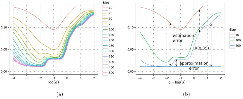
Figure 3: One step of CVST. Shown is the situation in steps= 10. Ê A model based on the first n data points is learned for each configuration (c1 tocK). Test errors
are calculated on the remaining data (dn+1 todN) and transformed into a binary
performance indicator via robust testing. Ë Traces of configurations are filtered via sequential analysis (cK−1 and cK are dropped). Ì The procedure checks
whether the remaining configurations perform equally well in the past and stops if this is the case. See Appendix B for a complete example run.
see in the evaluation section that all these effects are indeed helpful for an overall good performance of the CVST algorithm.
To find the top performing configurations for step s we look at the outcome of the learned model for each configuration, i.e., we subsequently take the rows of the pointwise performance matrix Pp into account and apply either the Friedman test (Friedman, 1937)
this step are separated from the rest of the configurations which will show a significantly different behavior on the individual data points.
More formally, the function topConfigurations described in Algorithm 2 takes the
pointwise performance matrixPp as input and rearranges the rows according to the mean
performances of the configurations yielding a matrix Pep. Now for k ∈ {2,3, . . . , K} we check, whether the first k configurations show a significantly different effect on the N −n
data points. This is done by executing either the Friedman test or the Cochran’s Q test on the submatrixPep[1 :k,1 : (N−n)] with the pre-specified significance levelα. If the test does not indicate a significant difference in the performance of thekconfigurations, we increment
kby one and test again until we find a significant effect. Suppose we find a significant effect at index ˜k. Since all previous tests indicated no significant effect for the ˜k−1 configurations we argue that the addition of the ˜kth configuration must have triggered the test procedure to indicate that in the set of these ˜k configurations is at least one configuration, which shows a significantly different behavior than all other configurations. Thus, we flag the configurations 1, . . . ,˜k−1 as top configurations and the remaining ˜k, . . . , K configurations as flop configurations. Note that this incremental procedure is a multiple testing situation, thus we apply the Bonferroni correction to the calculated p-values.
For the actual calculation of the test errors we apply an incremental model building process, i.e., the data added in each step on Line 22 increases the training data pool for each step by a set of size ∆. This would allow online algorithms to adapt their model also incrementally leading to even further speed improvements. The results of this first step are collected for each configuration in the trace matrixTS (see Figure 3, top right), which shows
the gradual transformation for the last 10 steps of the procedure highlighting the results of the last test. More formally,TS[c, s] is 1 iff configurationcis amongst the top configuration
in step s; ifc is not a top configuration in steps, the entryTS[c, s] is 0.
So this new column generated in step sin the trace matrix TS summarizes the
perfor-mance of all models learned on the first n data points in a robust way. Thus, the trace matrix TS records the history of each configuration in a binary fashion, i.e., whether it
performed as a top or flop configuration in each step of the CVST main loop. This leads to a robust transformation of the test errors of the configurations which can be modeled in the next step as a binary random variable with a success probability π indicating whether a configuration is amongst the top (high π) or the flop (lowπ) configurations.
4.2 Determining Significant Losers
(compare two production processes) or biological settings (stop bioassays as soon as the gathered data leads to a significant result). In this section we focus on the general idea of this approach while Section 5 gives details about how the CVST algorithm deals with potential switches in the winning probabilityπ of a given configuration.
The main idea of the sequential analysis framework is the following: One observes a sequence of i.i.d. Bernoulli variables B1, B2, . . ., and wants to test whether these variables
are distributed according to the hypotheses H0 : Bi ∼ π0 or the alternative hypotheses
H1 : Bi ∼ π1 with π0 < π1 denoting the according success probabilities of the Bernoulli
variables. Both significance levels for the acceptance of H1 and H0 can be controlled via
the user-supplied meta-parameters αl and βl. The test computes the likelihood for the so
far observed data and rejects one of the hypothesis when the respective likelihood ratio exceeds an interval controlled by the meta-parameters. It can be shown that the procedure has a very intuitive geometric representation, shown in Figure 3, lower left: The binary observations are recorded as cumulative sums at each time step. If this sum exceeds the upper red line L1, we accept H1; if the sum is below the lower red lineL0 we accept H0; if
the sum stays between the two red lines we have to draw another sample.
Wald’s test requires that we fix both success probabilities π0 and π1 beforehand. Since
our main goal is to use the sequential test to eliminate underperformers, we choose the parameters π0 and π1 of the test such thatH1 (a configuration wins) is postponed as long
as possible. This will allow the CVST algorithm to keep configurations until the evidence of their performances definitely shows that they are overall loser configurations. At the same time, we want to maximize the area where configurations are eliminated (region4H0
denoted by “LOSER” in Figure 3), rejecting as many loser configurations on the way as possible:
(π0, π1) = argmax
π00,π01
4H0(π
0
0, π
0
1, βl, αl) (1)
s.t.Sa(π00, π
0
1, βl, αl)∈(S−1, S]
with Sa(·,·,·,·) being the earliest step of acceptance of H1 marked by an X in Figure 3
andS denotes again the total number of steps. By using approximations from Wald (1947) for the expected number of steps the test will take, if the real success probability of the underlying process would indicate a constant winner (i.e., π = 1.0), we can fix Sa to the
maximal number of stepsS and solve Equation (1) as follows (see Appendix D for details):
π0 = 0.5∧π1 =
1 2
S
s 1−βl
αl
. (2)
Equipped with these parameters for the sequential test, we can check each remaining trace on Line 18 of Algorithm 1 in the functionisFlopConfiguration detailed in Algorithm 3
whether it is a statistically significant flop configuration (i.e., exceeds the lower decision boundary L0) or not.
approach taken in this step of the CVST algorithm this would amount to a change of the un-derlying success probabilityπof the configuration. Thus, the assumptions of the sequential testing framework would definitely be violated. We accommodate for this by introducing in Section 5.1 a so-calledsafety zone which acts as a safeguard against prematurely dropping of a configuration. Note that this safety zone can be controlled by the experimenter using the parametersαl and βl of the sequential test. If the experimenter chooses the right safety
zone the underlying success probabilities of the configuration remain stable after the safety zone and, hence, again will satisfy the preconditions of the sequential testing framework. So by ensuring no premature drop of a configuration in the safety zone we heuristically adapt the sequential test to the potential switch of underlying success probabilities. To give a complete account of the assumptions of the sequential analysis we will discuss potential violations of the independence of the top/flop variables and its implication for the CVST procedure in Section 5.
For details of the open sequential analysis please consult Wald (1947) or see for instance Wetherill and Glazebrook (1986) for a general overview of sequential testing procedures. Appendix D contains the necessary details needed to implement the proposed testing scheme for the CVST algorithm.
4.3 Early Stopping and Final Winner
Finally, we employ an early stopping rule (Line 20) which takes the lastwstop columns from
the trace matrix and checks whether all remaining configurations performed equally well in the past. In Figure 3 this submatrix of the overall trace matrixTS is shown for a value
of wstop = 4 for the remaining configurations after step 10. For the test, we again apply
the Cochran’s Q test (see Appendix C) in the similarPerformance procedure on the
submatrix ofTSas denoted in Algorithm 4. Figure 4 illustrates a complete run of the CVST
algorithm for roughly 600 configurations. Each configuration marked in red corresponds to a flop configuration and a black one to a top configuration. Configurations marked in gray have been dropped via the sequential test during the CVST algorithm. The small zoom-ins in the lower part of the picture show the last wstop remaining configurations during each
step which are used in the evaluation of the early stopping criterion. We can see that the procedure keeps on going if there is a heterogeneous behavior of the remaining configurations (zoom-in is mixed red/black). When all the remaining configurations performed equally well in the past (zoom-in is nearly black), the early stopping test does not see a significant effect anymore and the procedure is stopped.
Finally, in the procedure selectWinner, Line 23 and Algorithm 5, the winning
con-figuration is picked from the concon-figurations which have survived all steps as follows: For each remaining configuration we determine the rank in a step according to the average performance during this step. Then we average the rank over the last wstop steps and pick
the configuration which has the lowest mean rank. This way, we make most use of the data accumulated during the course of the procedure. By restricting our view to the last
wstop observations we also take into account that the optimal parameter might change with
100 200 300 400 500 600
1 2 3 4 5 6 7
Step
Configur
ation
Status
flop top out
s= 5 s= 6 s= 7
·
·
STOP!
50 100 150
3 4 5
20 40 60 80
4 5 6
20 40 60
5 6 7
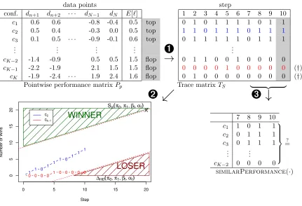
Figure 4: The upper plot shows a run of the CVST algorithm for roughly 600 configurations. At each step a configuration is marked as top (black), flop (red) or dropped (gray). The zoom-ins show the situation for step 5 to 7 without the dropped entries. The early stopping rule takes effect in step 7, because the remaining configurations performed equally well during step 5 to 7.
4.4 Meta-Parameters for the CVST
The CVST algorithm has a number of meta-parameters which the experimenter has to choose beforehand. In this section we give suggestions on how to choose these parameters. The parameterαcontrols the significance level for the test for similar behavior in each step of the procedure. We suggest to set this to the usual level ofα= 0.05. Furthermoreβl and
αl control the significance level of theH0 (configuration is a loser) andH1 (configuration is
a winner) respectively. We suggest an asymmetric setup by settingβl= 0.1, since we want
to drop loser configurations relatively fast and αl = 0.01, since we want to be really sure
when we accept a configuration as overall winner. Finally, we set wstop to 3 forS = 10 and
6 for S= 20, as we have observed that this choice works well in practice.
5. Properties of the CVST Algorithm
sta-ble regime. Given some assumptions about the top/flop variasta-bles we show that the CVST algorithm performs with high accuracy after a configuration has reached its stable regime. Additionally, we show how the CVST algorithm can be used to work best on a given time budget. Finally, we discuss some unsolved questions and give possible directions for future research.
5.1 Performance in a Stable Regime
As discussed in Section 2 the winning probability of a configuration might change if we feed the learning algorithm more data. Therefore, a reasonable algorithm exploiting the learning on subsets of the data must be capable of dealing with these difficulties and potential change points in the behavior of certain configurations. In this section we investigate some properties of the CVST algorithm which makes it particularly suitable for learning on increasing subsets of the data.
The first property of the open sequential test employed in the CVST algorithm comes in handy to control the overall convergence process and to assure that no configurations are dropped prematurely:
Lemma 1 (Safety Zone) Given the CVST algorithm with significance level αl, βl for
be-ing a top or flop configuration respectively, and maximal number of stepsS, and a configu-ration which loses for the first scp iterations, as long as
0≤ scp
S ≤
ssafe
S withssafe=
log βl 1−αl
log 2− qS 1−βl αl
and S≥
log1−βl
αl
/log 2
,
the probability that the configuration is dropped prematurely by the CVST algorithm is zero.
Proof The details of the proof are deferred to Appendix D.
The consequence of Lemma 1 is that the experimenter can directly control via the signif-icance levels αl, βl until which iteration no premature dropping should occur and therefore
guide the whole process into a stable regime in which the configurations will see enough data to show their real performance. Note that this property is a direct consequence of the sequential analysis framework and is used here to guide the test into a controlled region where we do not observe a premature dropping of configurations. Equation (2) ensures that we actually perform a meaningful test to discriminate a loser configuration (π0= 0.5)
from a winning configuration (π1 > π0). Thus, by adjusting the safety zone of the CVST
algorithm the experimenter can ensure that the configurations act according to the precon-ditions of the sequential testing framework introduced in Section 4.2, namely exhibiting a fixed probabilityπ of being a winner configuration at each step.
● ● ● ● ● ● ●
1 2 3 4 5 6 7 8 9 10 11 12 13 14 15 16 17 18 19 20
0
2
4
6
8
10
12
14
16
18
20
Step
Number of Wins
1 1 1
1 2
1 3 2
1 4 5
1 5 9 5
1 6 14 14
1 7 20 28
1 8 27 48 28
1 9 35 75 76
1 10 44 110 151 76
1 11 54 154 261 227
1 12 65 208 415 488 227
WINNER
LOSER
SAFETY−
ZONE
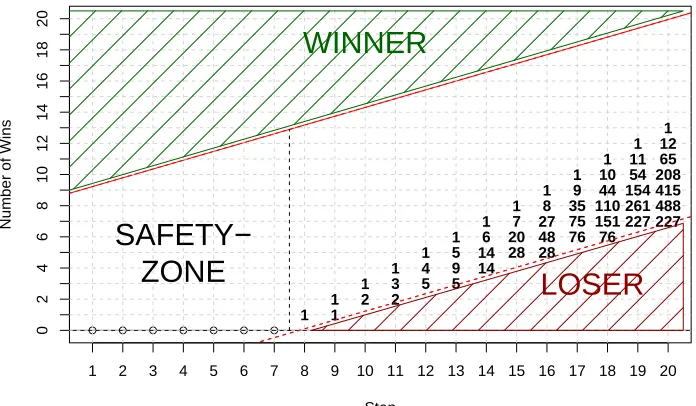
Figure 5: Visualization of the worst-case scenario for the error probability of the CVST algorithm: A global winner configuration is labeled as a constant loser until the safety zone is reached. Then we can calculate the probability that this configura-tion endures the sequential test by a recurrence scheme, which counts the number of remaining paths ending up in the non-loser region.
both the independence and identically distributed assumption of the sequential learning framework. We are fully aware that these assumptions are strong, yet, backed up by our extensive experimental evaluation in Section 6, we want to shed some light on why the CVST procedure shows such impressive speed-ups with small impact on the accuracy compared to ordinary cross-validation and even outperforms other model selection heuristics.
Hence, we define a stable configuration as a configuration which sticks to a certain probability π of being a winning configuration. So after having seen enough data to show its real behavior the robust transformation of the test error of the configuration inside the CVST algorithm (see Section 4.1) exhibits the properties of an i.i.d. Bernoulli variable and thus acts as a stable configuration in the subsequent steps of the CVST procedure. So a global winning configuration will be astableconfiguration with a probabilityππ0= 0.5.
Using these assumptions we can now take a look at the worst case performance of the
CVST algorithm. Suppose a global winning configuration has been constantly marked
as a loser up to the safety zone, because the amount of data available up to this point was not sufficient to show the superiority of this configuration. Given that the global winning configuration now sees enough data to be marked as a winning configuration by the binarization process throughout the next steps with probabilityπ, we can give an error bound of the overall process by solving specific recurrences.
safety zone of 7. Our approach to bound the error of the fast cross-validation now consists essentially in calculating the probability mass that ends up in the non-loser region. The following lemma shows how we can express the number of paths which lead to a specific point on the graph by a two-dimensional recurrence relation:
Lemma 2 (Recurrence Relation) Denote by Path(sR, sC) the number of paths, which
lead to the point at the intersection of rowsRand columnsC and lie above the lower decision boundaryL0 of the sequential test. Given the worst case scenario described above the number
of paths can be calculated as follows:
Path(sR, sC) =
1 if sR = 0∧c≤ssafe=
log1−βl αl
log 2−S
r
1−βl
αl
1 if sR =sC−ssafe
Path(sR, sC−1) + Path(sR−1, sC−1) if L0(c)< sR < sC−ssafe
0 otherwise.
Proof We split the proof into the four cases:
1. The first case is by definition: The configuration has a straight line of zeros up to the safety zonessafe.
2. The second case describes the diagonal path starting from the point (1, ssafe+ 1): By
construction of the paths (1 means diagonal up; 0 means one step to the right) the diagonal path can just be reached by a single combination, namely a straight line of ones.
3. The third case is the actual recurrence: If the given point is above the lower decision bound L0, then the number of paths leading to this point is equal to the number
of paths that lie directly to the left of this point plus the paths which lie directly diagonal downwards from this point. From the first paths this point can be reached by a direct step to the right and from the latter the current point can be reached by a diagonal step upwards. Since there are no other options than that by construction, this equality holds.
4. The last case describes all other paths, which either lie below the lower decision bound and therefore end up in the loser region or are above the diagonal and thus can never be reached.
This recurrence is visualized in Figure 5. Each number on the grid gives the number of valid, non-loser paths, which can reach the specific point. With this recurrence we are now able to prove a global, worst-case error probability of the fast cross-validation.
Theorem 3 (Error Bound of CVST for Stable Configuration) Suppose a global
S
Error Bound
0.05 0.10 0.15 0.20
10 15 20 25 30
π
0.9 0.925 0.95 0.975 0.99
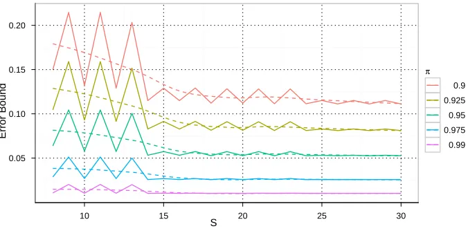
Figure 6: Error bound of the fast cross-validation as proven in Theorem 3 for different success probabilities π and maximal step sizes S. To mark the global trend we fitted a LOESS curve given as dotted line to the data.
to a stable winner configuration with a success probability ofπ π0 = 0.5. Then the error
that the CVST algorithm erroneously drops this configuration can be determined as follows:
P(reject π)≤1−
r
X
i=bL0(S)c+1
Path(i, S)πi(1−π)r−i withr=S−
log βl 1−αl
log 2− qS 1−βl αl
.
Proof The basic idea is to use the number of paths leading to the non-loser region to
calculate the probability that the configuration actually survives. This corresponds to the last column of the example in Figure 5. Since we model the outcome of the binarization process as a binomial variable with the success probability ofπ, the first diagonal path has a probability of πr. The next paths each have a probability of π(r−1)(1−π)1 and so on until the last viable paths are reached in the point (bL0(S)c+ 1, S). So the complete prob-ability of the survival of the configuration is summed up with the corresponding number of paths from Lemma 2. Since we are interested in the complementary event, we subtract the resulting sum from one, which concludes the proof.
Note that the early stopping rule does not interfere with this bound: The worst case is indeed that the process goes on for the maximal number of steps S, since then the probability mass will be maximally spread due to the linear lower decision boundary and the corresponding exponents are maximal. So if the early stopping rule terminates the process before reaching the maximum number of steps, the resulting error probability will be lower than our given bound.
The error bound for different success probabilities and the proposed sequential test with
αl = 0.01 andβl= 0.1 are depicted in Figure 6. First of all we can observe a relatively fast
S=10 S=20
0.0 0.2 0.4 0.6 0.8 1.0
● ●
● ● ●
● ● ● ●
● ● ● ● ● ● ● ● ●
● ● ● ●
● ● ● ● ● ●
2 4 6 8 5 10 15
Change Point
F
alse Negativ
e Rate
π
● 0.1 0.2 0.3 0.4 0.5
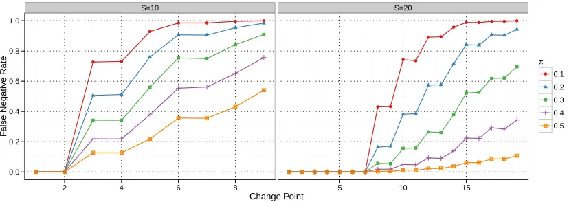
Figure 7: False negatives generated with the open sequential test for non-stationary config-urations , i.e., at the given change point the Bernoulli variable changes itsπbefore
from the indicated value to 1.0.
the error is marginal for the shown success probabilities, i.e., for instance for π = 0.95 the error nearly converges to the optimum of 0.05. Note that the oscillations especially for small step sizes originate from the rectangular grid imposed by the interplay of the Path-operator and the lower decision boundary L0 leading to some fluctuations. Overall, the chosen test
scheme allows us not only to control the safety zone but also has only a small impact on the error probability, which once again shows the practicality of the open sequential ratio test for the fast cross-validation procedure. By using this statistical test we can balance the need for a conservative retention of configurations as long as possible with the statistically controlled dropping of significant loser configurations with nearly no impact on the overall error probability.
Our analysis assumes that the experimenter has chosen the right safety zone for the learning problem at hand. For small data sizes it could happen that this safety zone was chosen too small, therefore the change point of the global winning configuration might lie outside the safety zone. While this will not occur often for today’s sizes of data sets we have analyzed the behavior of CVST under this circumstances to give a complete view of the properties of the algorithm. To get insight into the drop rate for the case when the experimenter underestimated the change point scp we simulate those switching
configura-tions by independent Bernoulli variables which change their success probability π from a chosenπbefore∈ {0.1,0.2, . . . ,0.5}to a constant 1.0 at a given change point. This behavior
essentially imitates the behavior of a switching configuration which starts out as a loser (i.e., up to the change point the trace will consist more or less of zeros) and after enough data is available turns into a constant winner.
The relative loss of these configurations for 10 and 20 steps is plotted in Figure 7 for different change points. The figure reveals our theoretical findings of Lemma 1 showing the corresponding safety zone for the specific parameter settings: For instance for αl =
c1
c2
..
. · · ·
c(1−r)K .. .
cK−1 · · · ·
cK
13
S3t 2
3
S3t sr×S (S−1)
3
S3 t S
3 S3t
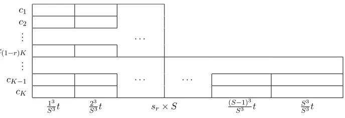
Figure 8: Approximation of the time consumption for a cubic learner. In each step we calculate a model on a subset of the data, so the model calculation timeton the full data set is adjusted accordingly. Aftersr×S steps of the process, we assume
a drop tor×K remaining configurations.
if the change point for all switching configurations occurs at step one or two, the CVST algorithm would not suffer from false positives. Similarly, for S = 20 the safety zone is 0.39×20 = 7.8. These theoretical results are confirmed in our simulation study, where the false negative rate is zero for sufficiently small change points for the open variant of the test. After that, there are increasing probabilities that the configuration will be removed. Depending on the success probability of the configuration before the change point, the resulting false negative rate ranges from mild forπ = 0.5 to relatively severe for
π = 0.1. The later the change point occurs, the higher the resulting false negative rate will be. Interestingly, if we increase the total number of steps from 10 to 20, the absolute values of the false negative rates are significantly lower. So even when the experimenter underestimates the actual change point, the CVST algorithm has some extra room which can even be extended by increasing the total number of steps.
5.2 Fast-Cross Validation on a Time Budget
While the CVST algorithm can be used out of the box to speed up regular cross-validation, the aforementioned properties of the procedure come in handy when we face a situation in which an optimal parameter configuration has to be found given a fixed computational budget. If the time is not sufficient to perform a full cross-validation or the amount of data that has to be processed is too big to explore a sufficiently spaced parameter grid with ordinary cross-validation in a reasonable time, the CVST algorithm can easily be adjusted to the specified time constraint. Thus, the experimenter is able to get the maximal number of model evaluations given the time budget available to judge which model is the best.
This is achieved by calculating a maximal steps parameter S which leads to a near coverage of the available time budget T as depicted in Figure 8. The idea is to specify an expected drop rate (1−r) of configurations and a safety zone bound ssafe. Then we
0 < sr < 1 to ensure that no configuration is dropped prematurely, the computational
demands of the CVST algorithm are approximated by the sum of the time needed before step ssafe involving the model calculation of all K configurations and after step ssafe for
r×K configurations with 0< r <1. As we will see in the experimental evaluation section, this assumption of a given drop rate of (1−r) leading to the form of time consumption as depicted in Figure 8 is quite common. The observed drop rate corresponds to the overall difficulty of the problem at hand.
Given the computation timetneeded to perform the model calculation on the full data set, we prove in Appendix E that the optimal maximum step parameter for a learner of time complexityf(n) =nm can be calculated as follows:
S=
m+ 1
4
2T−tK(1−r)sm r +tKr
((1−r)smr+1+r)tK
+ s
m+ 1
4
2T −tK(1−r)sm r +tKr
((1−r)smr+1+r)tK
2
−m(m+ 1)
12
(1−r)smr −1+r
(1−r)smr +1+r
.
After calculating the maximal number of steps S given the time budget T, we can use the results of Lemma 1 to determine the maximalβlgiven a fixedαl, which yields the requested
safety zone bound ssafe.
5.3 Discussion of Further Theoretical Analyses
In Section 2 we have noted that in order for the test performances to converge, the parameter configurations should be independent of the sample size. As shown in Appendix A this holds for a range of standard methods in machine learning. Yet, special care has to be taken to really ensure this assumption. For instance for kernel ridge regression one has to scale the ridge parameter during each step of the CVST algorithm to accommodate for the change in the learning set size (see the reference implementation in the official CRAN package named
CVST or the development version at https://github.com/tammok/CVST). The ν-Support
Vector Machine on the other hand directly incorporates this scaling of parameters which makes it a good fit for the CVST algorithm. Generally, it would be preferable to have this scaling automatically incorporated in the CVST algorithm such that the experimenter could plug-in his favorite method without the need to think about any scaling issues of hyper-parameters. Unfortunately, this is highly algorithm dependent and, thus, is an open problem for further research.
An additional concern to the practitioner is how to choose the correct size of the safety zone ssafe. If the training set does not contain enough data to get to a stable regime of
The similarity test introduced in Section 4.1 relies on two assumptions: First, the aver-aged loss function over the data not used for training in one step gives us a good indicator of the performance of a configuration. Second, well performing configurations show simi-lar behavior in classification or regression on the data not used for learning. While these assumptions definitely make sense, they encode a certain optimism of how the grid of con-figurations is populated: If we have too few concon-figurations as input to the procedure it might happen that some non-optimal configurations mask out the other, normally optimal, configurations just by chance. To overcome this problem we therefore would need a certain amount of redundancy in the configuration grid. Both the amount of redundancy and thus the similarity measure underlying this redundancy assumption are hard to grasp theoreti-cally, yet, it could lead to new ways to model the binary transformation of the performance of configurations in each step of the CVST algorithm.
There might be even further potential in the behavior of similar configurations that could be used in the CVST algorithm: If there is a notion of similarity between different configurations, it would be interesting to exploit this information and incorporate it into the CVST algorithm. For instance, one could add this kind of information in the function
topConfigurations of Algorithm 1 to average the result of similar configurations and,
hence, extend the pooling effect of the test already available for the data point dimension in the direction of configurations.
While the selection scheme explained in Section 4.2 deals with the fact of potential change points of a configuration, it is not clear how independent the individual entries of a trace for a given configuration are and how much these potential dependencies influence the power of the sequential testing framework. Preliminary experiments comparing the CVST algorithm as described in this paper and a version of the CVST algorithm where at each step the data pool is shuffled, thus, yielding always different data points for learning and evaluation, showed no significant differences between these two versions. This indicates that at least the potential dependencies introduced by the overlap of learning sets due to subsequent addition of data points do not interfere with the dependency assumption of the sequential testing framework. We will see in the evaluation section that the CVST procedure in its current form shows excellent behavior throughout a wide range of data sets; yet, further research of the theoretical properties of CVST might yield even better procedures in the future.
6. Experiments
Before we evaluate the CVST algorithm on real data, we investigate its performance on controlled data sets. Both for regression and classification tasks we introduce special tai-lored data sets to highlight the overall behavior and to stress-test the fast cross-validation procedure. To evaluate how the choice of learning method influences the performance of the CVST algorithm, we compare kernel logistic regression (KLR) against a ν-Support Vector Machine (SVM) for classification problems and kernel ridge regression (KRR) versus ν -SVR for regression problems each using a Gaussian kernel (see Roth, 2001; Sch¨olkopf et al., 2000). In all experiments we use a 10 step CVST with parameter settings as described in Section 4.4 (i. e. α= 0.05, αl = 0.01, βl = 0.1, wstop = 3) to give us an upper bound of the
● ● ● ● ● ● ● ● ● ● ● ● ● ● ● ● ● ● ● ● ● ● ● ● ● ● ● ● ● ● ● ● ● ● ● ● ● ● ● ● ● ● ● ● ● ● ● ● ● ● ● ● ● ● ● ● ● ● ● ● ● ● ● ● ● ● ● ● ● ● ● ● ● ● ● ● ● ● ● ● ● ● ● ● ● ● ● ● ● ● ● ● ● ● ● ● ● ● ● ● ● ● ● ● ● ● ● ● ● ● ● ● ● ● ● ● ● ● ● ● ● ● ● ● ● ● ● ● ● ● ● ● ● ● ● ● ● ● ● ● ● ● ● ● ● ● ● ● ● ● ● ● ● ● ● ● ● ● ● ● ● ● ● ● ● ● ● ● ● ● ● ● ● ● ● ● ● ● ● ● ● ● ● ● ● ● ● ● ● ● ● ● ● ● ● ● ● ● ● ● ● ● ● ● ● ● ● ● ● ● ● ● ● ● ● ● ● ● ● ● ● ● ● ● ● ● ● ● ● ● ● ● ● ● ● ● ● ● ● ● ● ● ● ● ● ● ● ● ● ● ● ● ● ● ● ● ● ● ● ● ● ● ● ● ● ● ● ● ● ● ● ● ● ● ● ● ● ● ● ● ● ● ● ● ● ● ● ● ● ● ● ● ● ● ● ● ● ● ● ● ● ● ● ● ● ● ● ● ● ● ● ● ● ● ● ● ● ● ● ● ● ● ● ● ● ● ● ● ● ● ● ● ● ● ● ● ● ● ● ● ● ● ● ● ● ● ● ● ● ● ● ● ● ● ● ● ● ● ● ● ● ● ● ● ● ● ● ● ● ● ● ● ● ● ● ● ● ● ● ● ● ● ● ● ● ● ● ● ● ● ● ● ● ● ● ● ● ● ● ● ● ● ● ● ● ● ● ● ● ● ● ● ● ● ● ● ● ● ● ● ● ● ● ● ● ● ● ● ● ● ● ● ● ● ● ●● ● ● ● ● ● ● ● ● ● ● ● ● ● ● ● ● ● ● ● ● ● ● ● ● ● ● ● ● ● ● ● ● ● ● ● ● ● ● ● ● ● ● ● ● ● ● ● ● ● ● ● ● ● ● ● ● ● ● ● ● ● ● ● −1 0 1
0 10 20 30
x y label ● ● +1 0 ● ● ● ● ● ● ● ● ● ● ● ● ● ● ● ● ● ● ● ● ● ● ● ● ● ● ● ● ● ● ● ● ● ● ● ● ● ● ● ● ● ● ● ● ● ● ● ● ● ● ● ● ● ● ● ● ● ● ● ● ● ● ● ● ● ● ● ● ● ● ● ● ● ● ● ● ● ● ● ● ● ● ● ● ● ● ● ● ● ● ● ● ● ● ● ● ● ● ● ● ● ● ● ● ● ● ● ● ● ● ● ● ● ● ● ● ● ● ● ● ● ● ● ● ● ● ● ● ● ● ● ● ● ● ● ● ● ● ● ● ● ● ● ● ● ● ● ● ● ● ● ● ● ● ● ● ● ● ● ● ●● ● ● ● ● ● ● ● ● ● ● ● ● ● ● ● ● ● ● ● ● ● ● ● ● ● ● ● ● ● ● ● ● ● ● ● ● ● ● ● ● ● ● ● ● ● ● ● ● ● ● ● ● ● ● ● ● ● ● ● ● ● ● ● ● ● ● ● ● ● ● ● ● ● ● ● ● ● ● ● ● ● ● ● ● ● ● ● ● ● ● ● ● ● ● ● ● ● ● ● ● ● ● ● ● ● ● ● ● ● ● ● ● ● ● ● ● ● ● ● ● ● ● ● ● ● ● ● ● ● ● ● ● ● ● ● ● ● ● ● ● ● ● ● ● ● ● ● ● ● ● ● ● ● ● ● ● ● ● ● ● ● ● ● ● ● ● ● ● ● ● ● ● ● ● ● ● ● ● ● ● ● ● ● ● ● ● ● ● ● ● ● ● ● ● ● ● ● ● ● ● ● ● ● ● ● ● ● ● ● ● ● ● ● ● ● ● ● ● ● ● ● ● ● ● ● ● ● ● ● ● ● ● ● ● ● ● ● ● ● ● ● ● ● ● ● ● ● ● ● ● ● ● ● ● ● ● ● ● ● ● ● ● ● ● ● ● ● ● ● ● ● ● ● ● ● ● ● ● ● ● ● ● ● ● ● ● ● ● ● ● ● ● ● ● ● ● ● ● ● ● ● ● ● ● ● ● ● ● ● ● ● ● ● ● ● ● ● ● ● ● ● ● ● ● ● ● ● ● ● ● ● ● ● ● ● ● ● ● −0.5 0.0 0.5 1.0
−2 0 2
x
y
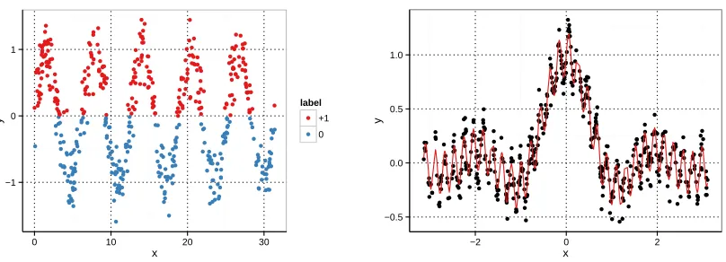
Figure 9: Thenoisy sine (left) andnoisy sinc data set (right).
number of steps or increasingβl. From a practical point of view we believe that the settings
studied are highly realistic.
6.1 Artificial Data Sets
To assess the quality of the CVST algorithm we first examine its behavior in a controlled setting. We have seen in our motivation section that a specific learning problem might have several layers of structure which can only be revealed by the learner if enough data is available. For instance in Figure 2(a) we can see that the first optimal plateau occurs at
σ = 0.1, while the real optimal parameter centers aroundσ= 0.01. Thus, the real optimal choice just becomes apparent if we have seen more than 200 data points.
In this section we construct a learning problem both for regression and classification tasks which could pose severe problems for the CVST algorithm: If it stops too early, it will return a suboptimal parameter set. We evaluate how different intrinsic dimensionalities of the data and various noise levels affect the performance of the procedure. For classification tasks we use the noisy sine data set, which consists of a sine uniformly sampled from a range controlled by the intrinsic dimensionality d:
y= sin(x) + with∼ N(0, n2), x∈[0,2πd], n∈ {0.25,0.5}, d∈ {5,50,100}.
The labels of the sampled points are just the sign of y. An example for d= 5, n= 0.25 is plotted in the left subplot of Figure 9. For regression tasks we devise the noisy sinc data set, which consists of a sinc function overlayed with a high-frequency sine:
y= sinc(4x) +sin(15dx)
5 +with∼ N(0, n
2), x∈[−π, π], n∈ {0.1,0.2}, d∈ {2,3,4}.
n=0.25 n=0.50
● ● ● ● ●
● ● ●
● ●
● ●
● ● ●
●
● ●
● ● ●
● ●
● ● ●
● ● ● ●
●
● ●
● ● ●
●
● ●
−0.025 0.000 0.025 0.050 0.075
d=5 d=50 d=100 d=5 d=50 d=100
MSE F
ast CV − MSE Full CV
Method
KLR SVM
n=0.25 n=0.50
● ●
● ●
0 25 50 75 100
d=5 d=50 d=100 d=5 d=50 d=100
Time Full CV / Time F
ast CV
Method
KLR SVM
Figure 10: Difference in mean square error (left) and relative speed gain (right) for the
noisy sine data set.
for each method (log10(σ) ∈ {−3,−2.9, . . . ,3} and ν ∈ {0.05,0.1, . . . ,0.5} for SVM/SVR and log10(λ) ∈ {−7,−6, . . .2} for KLR/KRR, respectively). This process is repeated 50 times to gather sufficient data for an interpretation of the overall process. Apart from recording the difference in mean square error (MSE) of the learner selected by normal cross-validation and by the CVST algorithm we also look at the relative speed gain. Note that we have encoded the classes as 0 and 1 for the classification experiments so the MSE corresponds to the misclassification rate of the learner. So the difference in MSE gives us a good measurement of the impact of using the CVST algorithm for both classification and regression experiments.
The results for thenoisy sine data set can be seen in Figure 10. The left boxplots show the distribution of the difference in MSE of the best parameter determined by CVST and normal cross-validation. In the low noise setting (n= 0.25) the CVST algorithm finds the same optimal parameter as the normal cross-validation up to the intrinsic dimensionality of
d= 50. For d= 100 the CVST algorithm gets stuck in a suboptimal parameter configura-tion yielding an increased classificaconfigura-tion error compared to the normal cross-validaconfigura-tion. This tendency is slightly increased in the high noise setting (n= 0.5) yielding a broader distri-bution. The classification method used seems to have no direct influence on the difference, both SVM and KLR show nearly similar behavior. This picture changes when we look at the speed gains: While the SVM nearly always ranges between 10 and 20, the KLR shows a speed-up between 20 and 70 times. The variance of the speed gain is generally higher compared to the SVM which seems to be a direct consequence of the inner workings of KLR: The main loop performs at each step a matrix inversion of the whole kernel matrix until the calculated coefficients converge. Obviously this convergence criterion leads to a relative wide-spread distribution of the speed gain when compared to the SVM performance.