Learning Symbolic Representations of Hybrid Dynamical Systems

Learning Symbolic Representations of Hybrid Dynamical Systems

Daniel L. Ly DLL73@CORNELL.EDU

Hod Lipson∗ HOD.LIPSON@CORNELL.EDU

Sibley School of Mechanical and Aerospace Engineering Cornell University

Ithaca, NY 14853, USA

Editor:Yoshua Bengio

Abstract

A hybrid dynamical system is a mathematical model suitable for describing an extensive spec-trum of multi-modal, time-series behaviors, ranging from bouncing balls to air traffic controllers. This paper describes multi-modal symbolic regression (MMSR): a learning algorithm to construct non-linear symbolic representations of discrete dynamical systems with continuous mappings from unlabeled, time-series data. MMSR consists of two subalgorithms—clustered symbolic regression, a method to simultaneously identify distinct behaviors while formulating their mathematical ex-pressions, and transition modeling, an algorithm to infer symbolic inequalities that describe binary classification boundaries. These subalgorithms are combined to infer hybrid dynamical systems as a collection of apt, mathematical expressions. MMSR is evaluated on a collection of four synthetic data sets and outperforms other multi-modal machine learning approaches in both accuracy and in-terpretability, even in the presence of noise. Furthermore, the versatility of MMSR is demonstrated by identifying and inferring classical expressions of transistor modes from recorded measurements.

Keywords: hybrid dynamical systems, evolutionary computation, symbolic piecewise functions,

symbolic binary classification

1. Introduction

The problem of creating meaningful models of dynamical systems is a fundamental challenge in all branches of science and engineering. This rudimentary process of formalizing empirical data into parsimonious theorems and principles is essential to knowledge discovery as it provides two integral features: first, the abstraction of knowledge into insightful concepts, and second, the nu-merical prediction of behavior. While many parametric machine learning techniques, such as neural networks and support vector machines, are numerically accurate, they shed little light on the inter-nal structure of a system or its governing principles. In contrast, symbolic and ainter-nalytical models, such as those derived from first principles, provide such insight in addition to producing accurate predictions. Therefore, the automated the search for symbolic models is an important challenge for machine learning research.

Traditionally, dynamical systems are modeled exclusively as either a continuous evolution, such as differential equations, or as a series of discrete events, such as finite state machines. However, systems of interest are becoming increasingly complex and exhibit a non-trivial interaction of both continuous and discrete elements, which cannot be modeled exclusively in either domain (Lunze,

2002). As a result, hybrid automata, mathematical models which incorporate both continuous and discrete components, have become a popular method of describing a comprehensive range of real-world systems as this modeling technique is perfectly suited for systems that transition between dis-tinct qualitative behaviors. Hybrid dynamical models have been successfully applied to succinctly describe systems in a variety of fields, ranging from the growth of cancerous tumors (Anderson, 2005) to air traffic control systems (Tomlin et al., 1998).

Although it is plausible to construct hybrid models from inspection and first principles, this process is laborious and requires significant intelligence and insight since each subcomponent is itself a traditional modeling problem. Furthermore, the relationships between every permutation of the subcomponents must be captured, further adding to the challenge. Thus, the ability to automate the modeling of hybrid dynamical systems from time-series data will have a profound affect on the growth and automation of science and engineering.

Despite the variety of approaches for inferring models of time-series data, none are particularly well-suited for building apt descriptions of hybrid dynamical systems. Traditional approaches as-sume an underlying form and regress model parameters; some approaches conform the data using prior knowledge (Ferrari-Trecate et al., 2003; Vidal et al., 2003; Paoletti et al., 2007), while others are composed of generalized, parametric, numerical models (Chen et al., 1992; Bengio and Fras-coni, 1994; Kosmatopouous et al., 1995; Le et al., 2011). Although numeric approaches may be capable of predicting behavior with sufficient accuracy, models of arbitrary systems often require vast numbers of parameters, which obfuscates the interpretability of the inferred model (Breiman, 2001). This trade-off between accuracy and complexity for parametric models is in direct opposition to a fundamental aspect of scientific modeling—abstracting relationships that promote the formu-lation of new theorems and principles. Thus, constructing symbolic models of hybrid dynamical systems which can be easily and naturally interpreted by scientists and engineers is a key challenge. The primary contribution of this paper is a novel algorithm, called multi-modal symbolic regres-sion (MMSR), to learn symbolic models of discrete dynamical systems with continuous mappings, as an initial step towards learning hybrid automata. It is a data-driven algorithm that formulates symbolic expressions to describe both the continuous behavior and discrete dynamics of an arbi-trary system. Two general learning processes are presented: the first algorithm, clustered symbolic regression (CSR), generates symbolic models of piecewise functions and the second algorithm, transition Modeling (TM), searches for symbolic inequalities to model transition conditions. These processes are then applied to a hybrid dynamical systems framework and are used to reliably model a variety of classical problems. MMSR is also applied to infer the modes of operation of a field-effect transistor, similar to those derived from first principles, from measured observations.

The remainder of this paper is organized as follows: Section 2 provides a brief introduction to hybrid dynamical systems, as well as a description of the relevant work in related fields. Section 3 introduces the theoretical background and implementation details of MMSR, with CSR and SR described in Section 3.2 and 3.3, respectively. Section 4 compares MMSR to traditional machine learning algorithms on four synthetic data sets and presents the inferred transistor model. The paper is concluded in Section 5.

2. Background

described and formulated as the inference target. This is followed by a discussion of the related work in learning hybrid dynamical systems.

2.1 Hybrid Automata

Due to the its inherent complexity, hybrid dynamical systems have only recently emerged as an area of formal research. Consequently, there is a lack of a common framework, terminology and defini-tion that is universally adopted (Henzinger, 1996; van der Schaft and Schumacher, 2000; Branicky, 2005). Our work uses a popular model called the hybrid automata, which extends the finite au-tomata model to include continuous dynamics. The evolution of the system is deterministic. Each automata,

H

, is defined as a 5-tuple,

H

= (

W

,

X

,

M

,

F

,

T

), with the following definitions:

(a) (b)

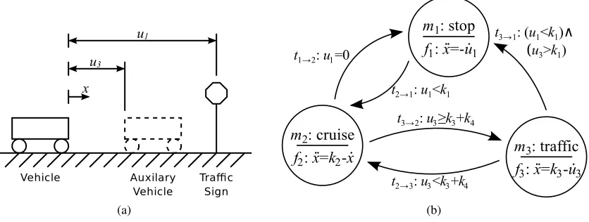
Figure 1: An example of a hybrid automata model for a simple, 1D driverless car. A schematic of the system is shown in a) and the system diagram represented as a directed graph is shown in b).

W

consists of two inputs, u1 andu3, which corresponds to the distance

to the nearest sign and vehicle, respectively; while

X

consists of the state variables x and ˙x, which describe the vehicle’s position and velocity.

M

consists of three modes,

{m1,m2,m3}, which represent distinct behaviors corresponding to whether the vehicle is

approaching a traffic sign, cruising or driving in traffic; and the behaviors for each mode is described by{f1,f2,f3}. There are five transitions events, each represented by a Boolean

condition.

•

W

defines a communication space for whichexternal variables,w, can take their values. The external variables can be further subdivided intoinput variables,u∈Ra, andoutput variables, y∈Rb, where

W

={u,y}.

•

X

defines a continuous space for which continuousstate variables, x∈Rc, can take their values.

•

F

defines a countable, discrete set of first-order, coupled, differential-algebraic equations (DAE). Each equation defines relationship between the state variables, their first-order time derivatives and the inputs:

fk(x,x˙,w) =0

and the solution to these DAE are called theactivitiesorbehaviorsof the mode. Each mode, mk, is defined by its corresponding behavior, fk, and the solution to the DAE defines the

continuous evolution of the system when it is in that mode.

•

T

defines a countable, discrete set of transitionsorevents, wheretk→k′ denotes a Boolean expression that represents the condition to transfer from modek to modek′. If none of the transition conditions are satisfied, then the hybrid automata remains in the current mode and the state variables evolves according to the specified behavior. These are represented as di-rected edges in the system diagram. ForKmodes, there are must be at leastK−1 transitions and at most K2 transitions. The transitions defines the discrete evolution of the system by describing how the mode is updated over time.

The challenge in modeling hybrid automata arises from the property that the latent “state” of a hybrid automata depends on both the discrete mode,mk, as well as the continuous state space vector,

x. As with all dynamical systems, the evolution of the system depends on the initial condition of the latent modes as well as the input variables. An example of a hybrid automata model for a simple, 1D driverless car is illustrated in Figure 1.

2.2 Discrete Dynamical System with Continuous Mappings

Hybrid automata are complex models which are capable of describing multi-modal behavior and latent continuous and discrete variables. To restrict the scope of the general problem, a number of assumptions are applied:

1. Each behavior is unique—No two behaviors are the same for any combination of modes: fi(·)6= fj(·),∀mi6=mj.

2. There are no continuous state space variables—All continuous states are directly observable and, thus, the behaviors are defined as strictly input-output relationships,y=f(u), as opposed to DAEs,y= f(x,x˙,u).

3. The number of discrete modes is known—The cardinality of the modes,|M|=K, is provided.

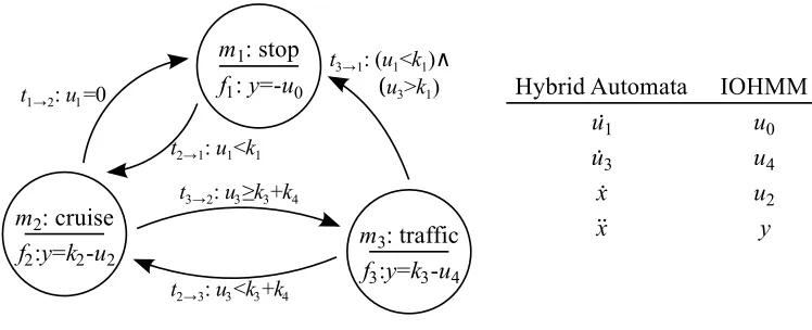
These assumptions describe a continuous-discrete hybrid system that evolves with discrete dy-namics but contains continuous input-output relationships. This formulation makes the symbolic inference tractable while also providing a first step to the general solution of inferring hybrid au-tomata. With the exception of assumption 3, each assumption defines a subset of models. If assump-tion 1 is relaxed, then the model becomes a continuous input-output hidden Markov model (Bengio and Frasconi, 1994). If assumption 2 is further relaxed, then the model becomes the standard hybrid automata described in Section 2.1.

The resulting discrete dynamical system with continuous mappings are defined as a 4-tuple,

observed input as well as the latent mode variable. Furthermore, the evolution of the latent mode variable is dependent on the input via the transition conditions. To continue with the driverless car example, a hybrid automata is transformed into the desired model by converting the mode and differentiated inputs as explicit inputs and outputs (Figure 2).

Figure 2: A conversion of the 1D driverless car hybrid automata as a discrete dynamical model with continuous mappings. The system diagram and variable conversion are shown.

2.3 Related Work

Although there is little work in the automated, data-driven construction of models of hybrid dynam-ical systems whose components are expressed in symbolic mathematics, there are many machine learning approaches that are capable of describing and predicting the behavior of multi-modal, time-series data via alternate approaches.

Interest in hybrid dynamical systems is primarily spurred by the control systems community and consequently, they have proposed a variety of approaches to infer dynamical systems. One approach addresses the problem of modeling discrete-time hybrid dynamical systems by reducing the problem to switched, piecewise affine models (Ferrari-Trecate et al., 2003; Vidal et al., 2003), and procedures using algebraic, clustering-based, Bayesian, and bounded-error methods have been proposed (Paoletti et al., 2007). This modeling technique imposes a linear form to the system’s dynamics, which substantially simplifies the modeling but limits the explanatory range of such models by enforcing linear approximations to non-linear systems.

Recurrent neural networks (RNNs) have been a popular approach for modeling time-series data. The input-output relationship of a general, continuous dynamical system has been modeled with RNNs (Kosmatopouous et al., 1995) and it has also been shown that recurrent neural networks are capable of modeling finite state machines (Horne and Hush, 1996). However, there has been no reported work on specifically modeling discrete dynamical systems with continuous inputs and outputs. RNNs are also restricted by their parametric nature, often resulting in dense and uninter-pretable models.

Consequently, there has been significant interest in extracting rules from parametric, recurrent neural networks to build a formal, symbolic model and providing an important layer of knowledge abstraction (Omlin and Giles, 1993, 1996a,b; Vahed and Omlin, 2004). However, a recent review of this work suggests that there is limited progress in handling RNNs with non-trivial complexity (Jacobsson, 2006).

The learning of input-output hidden Markov machines has been previously studied by Bengio and Frasconi (1994), which uses architecture based on neural networks to predict both the output of each mode as well as the transition conditions. The generalized expectation-maximization algorithm is used to optimize the parameters of in each of neural networks. Although the original work was implemented on grammatical inference with discrete inputs and outputs, the framework has since been adapted to several applications in the continuous domain (Marcel et al., 2000; Gonzalez et al., 2005). However, these approaches also rely on complex parametric neural network models.

Our technique attempts to resolve these various challenges by building models of hybrid dy-namical systems that uses non-linear symbolic expressions for both the behaviors as well as the transitions. Rather than imposing a linear structure or using parametric models, symbolic expres-sions are inferred to provide a description that is in the natural, mathematical representation used by scientists and engineers.

3. Multi-Modal Symbolic Regression Learning Algorithm

This section begins with a formalization of the learning problem. This is followed by the description of two, general algorithms: clustered symbolic regression and transition modelling. The section is concluded by combining both subalgorithms within a hybrid dynamics framework to form the multi-modal symbolic regression algorithm.

3.1 Problem Formalization

The goal of the algorithm is to infer a symbolic discrete dynamics model with continuous mappings from time-series data, where symbolic mathematical expressions are learned for both the behaviors as well as the transition events. Consider a dynamical system that is described by:

mn=T(mn−1,un),

y_n=F(mn,un) =

   

  

F1(un) , ifmn=1

..

. , ...

FK(un) , ifmn=K

whereun∈Rpis the input vector at timen,yn∈Rris the output vector, andmn∈M={1,2, . . . ,K}

The goal is to infer a multi-modal, input-output model that minimizes the normalized, negative log probability of generating the desired output vector under a mixture of Laplacians model,E, over the time series:

E= 1

N

N

∑

n=1 −ln

K

∑

k=1 γk,ne−

||yn−ˆ_yk,n|| σy

!

(1)

whereγk,n=p(mn=k)or the probability that the system is in modek, ˆyk,nis the output of function

Fk(un), andσyis the standard deviation of the output data.

This error metric is adapted from related work by Jacobs et al. (1991) on mixtures of local experts, but with the assumption of Laplacian, as opposed to Gaussian, distributions. The Lapla-cian distribution was chosen due to its relationship to absolute error, rather than squared error for Gaussian distributions. Note that for true mode probabilities or uni-modal models, this error metric indeed reduces to normalized, mean absolute error. Mean absolute error was preferred over squared error as is it more robust to outlier errors that occur due to misclassification.

To learn symbolic models of discrete dynamical systems with continuous mappings, the multi-modal symbolic regression (MMSR) algorithm is composed of two general algorithms: clustered symbolic regression (CSR) and transition modelling (TM). CSR is used to cluster the data into symbolic subfunctions, providing a method to determine the modal data membership while also in-ferring meaningful expressions for each subfunction. After CSR determines the modal membership, TM is then applied to find symbolic expressions for the transition conditions.

This algorithm varies from traditional learning approaches for hidden Markov model; conven-tional Baum-Welch or forward-backward algorithms are insufficient for dealing with the input-output relationships and transition conditions. Bengio and Frasconi (1994) approached the learning challenge by introducing the generalized expectation-maximization (GEM) to find the optimum parameters for the input-output functions and transition conditions simultaneously. However, for non-trivial, continuous systems, the GEM approach is likely to settle on local optima due to the inability of transition modelling to discriminate distinct modes. By dividing the problem into the CSR and TM subdomains, our approach leverages the property that each behavior is unique to infer accurate and consistent hybrid dynamical systems.

3.2 Clustered Symbolic Regression

The first algorithm is clustered symbolic regression (CSR), which involves using unsupervised learning techniques to solve the challenging issue of distinguishing individual functions while si-multaneously infers a symbolic model for each of them. This novel algorithm is presented as a generalized solution to learning piecewise functions, distinct from the hybrid dynamics framework.

3.2.1 PROBLEMDEFINITION

Consider the following, generalized piecewise function:

y_n= f(un) =

   

  

f1(un) , ifdn∈D1

..

. , ...

fK(un) , ifdn∈DK

whereun∈Rpis the observable input vector at indexn,yn∈Rris the output vector,dn∈Rqis the

domain input vector andDis a set of mutually exclusive membership subdomains. The domain input vector can be composed of both the observable variables,un, as well as latent variables, allowing for

latent subdomains definitions. Given the number of subdomains,K, infer a model that minimizes the within-domain, absolute error,E:

ECSR=

N

∑

n=1 K

∑

k=1

γk,n||yn−yˆn|| (2)

whereγk,nis the probability that the input-output pair belongs to the subdomainDkand ˆynare model

predictions of the output at timen.

In essence, this formulation is an unsupervised clustering problem. However, unlike traditional clustering problems, each cluster is represented by a symbolic expression and there is no prior knowledge regarding the structure of these submodels. There has been no reported work on mixture models where each component model is dependent on an arbitrary functional of the input; con-ventional mixture models assume that each cluster belongs to the same fixed-structure, parametric family of distributions (Bishop, 2006).

3.2.2 SYMBOLICREGRESSION

The first component of CSR is symbolic regression (SR): an genetic programming algorithm that is capable of reliably inferring symbolic expressions that models a given data set (Cramer, 1985; Dickmanns et al., 1987; Koza, 1992; Olsson, 1995). Provided with a collection of building blocks and a fitness metric, SR attempts to find the combination of primitives that best maximizes the stated fitness function.

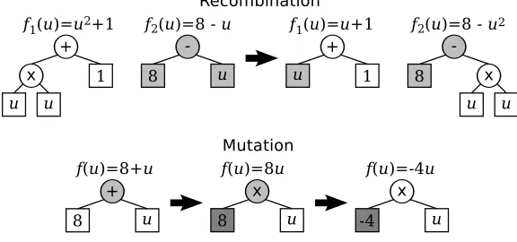
SR is a population-based, heuristic search algorithm which uses biologically-inspired evolution-ary techniques to efficiently explore a boundless search space. The process begins with a random population of candidate expressions. A fitness metric, such as squared or absolute error, is used to rank each candidate based on its ability to model the data set. The best candidates are selected to produce the next generation of expressions, through evolution-inspired techniques such as stochastic recombination and mutation. This process is summarized in Figure 3.

Figure 3: Flowchart describing the symbolic regression algorithm.

Figure 4: Symbolic expressions represented as tree structures, with examples of recombination and mutation operations.

operations. Furthermore, the tree structure is extremely amenable to the evolutionary processes of recombination and mutation through tree manipulations (Figure 4).

SR was chosen as the modeling algorithm because it provides three unique advantages. First, SR includes form and structure as part of the inference problem. Free form expressions are generated by rearranging primitives in a boundless tree structure, resulting in a rich range of possible expressions. In contrast, parametric models constrict their solution space to sums of basis and transfer functions. Next, SR produces solutions that are easily interpreted. Unlike other machine learning algo-rithms which tweak a vast collection of intangible numerical parameters, symbolic expressions are the foundation of mathematical notation and often provide key insight into the fundamental rela-tionships of such models.

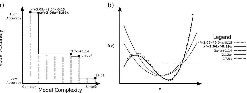
Figure 5: An example of the set of solutions provided by symbolic regression. a) The Pareto optimal solutions (in black) are expressions that have the best accuracy for all models of equal or lower complexity. Suboptimal solutions generated by SR are in grey. b) A plot of the non-dominated solutions with the corresponding the data set. The true model is in bold text, while the remaining solutions are either under- or overfit.

overfitting occurs by inferring a model with greater complexity than the ground truth—for example, a cubic model is used to fit a quadratic function. Thus, there is a fundamental trade-off between the accuracy and complexity of a candidate model, where overfitting incurs additional complexity to accurately model the noise contributions in the data.

Instead of simply reporting the most accurate model found by SR, which is susceptible to over-fitting, the inherent population dynamics is leveraged to provide a multi-objective approach to deal-ing with overfittdeal-ing. By design, SR generates numerous candidate models with varydeal-ing degrees of complexity and accuracy. Rather than considering every considering every generated expression as a candidate model, individual expressions are compared against a continuously updated, multi-objective record. This approach, called Pareto optimization, forms a set of non-dominated solutions which provide the best fitness for a given complexity (Figure 5). This method reformulates the prob-lem of overfitting as model selection along the accuracy and complexity trade-off, a property later exploited by CSR to reliably find solutions. As Pareto optimization is a post-processing technique that analyzes expressions only after they have been generated by SR, it does not interfere with the underlying search process.

Algorithm 1Generalized EM

input → observed data - X

output → model parameters - θ

initialize model parameters - θold while convergence is not achieved :

# expectation step

compute probability of observing latent variables - p(Z|X,θold) # maximization step

compute new model parameters - θnew=arg maxθ∑Zp(Z|X,θold)lnp(X|Z,θ) update model parameters - θold=θnew

return model parameters θold

3.2.3 EXPECTATION-MAXIMIZATION

The second component of CSR is the expectation-maximization (EM) algorithm: a machine learn-ing algorithm that searches for the maximum likelihood estimates of model parameters and latent variables. Formally, the EM solves the following problem: given a joint distribution p(X,Z|θ)over observed variables X and latent variablesZ, governed by the model parametersθ, determine the parameter values that maximize the likelihood function p(X|θ)(Dempster et al., 1977).

The EM algorithm is an iterative two-step process, which begins with initially random model parameters. In the expectation step, the expected value of the latent variables is determined by calculating the log-likelihood function given the current model parameters. This is followed by the maximization step, where the model parameters are chosen in order to maximize the expected value given the latent variables. Each cycle of EM increases the incomplete-data log-likelihood, unless it is already at a local optimum. The implementation details of EM are summarized in Algorithm 1.

The EM algorithm is a popular framework for a variety of mixture models, including mixture of Gaussians, mixture of Bernoulli distributions and even Bayesian linear regression (Bishop, 2006). Although evolutionary computation has been applied to the EM framework (Martinez and Virtia, 2000; Pernkopf and Bouchaffra, 2005) , the focus has been on exploring different optimization approaches in the maximization step for mixture of Gaussians, as opposed to investigating different types of models found through evolutionary computation.

3.2.4 CLUSTEREDSYMBOLIC REGRESSION

The clustered symbolic regression (CSR) is a novel algorithm that is capable of finding symbolic expressions for piecewise functions. By applying an EM framework to SR, this algorithm deter-mines both the model parameters, mathematical expressions and the corresponding variances for each subfunction, as well as the latent variables, the membership of each data point, for a piecewise function.

To aid in the formulation of the algorithm, the SR optimization is interpreted in a statistical framework where the output of each subfunction defines the expected value conditional on the input and state, fk(un) =E[yn|mk,un], wheremkis 1 ifdk∈Dkand 0 otherwise. Assuming that the noise

follows a Gaussian distribution, then the following definition is obtained:

pk(yn|un) =

N

yn|fk(un),σ2k

where

N

x|µ,σ2

defines a Gaussian distribution overxwith a meanµand varianceσ2_.

The expectation step consists of evaluating the expected membership values using the current model. Using the probabilistic framework for defining functions (Equation 3), the probability of membership,γk,n, of an input-output pair to a function fkis:

γk,n=

N

y_n|fk(un),σ2_k

∑K_k=1

N

y_n|fk(un),σ2k

. (4)

Note that the membership probability reinforces exclusivity—given two subfunctions with the same expression, the model with lower variance has stronger membership values over the same data. This property is advantageous given the assumption that each behavior is unique; as one subfunction becomes increasingly certain as a result of a decreased variance, the other subfunctions are forced to model the remaining data.

Next, the Maximization Step consists of finding the expressions for each behavior and vari-ances that best explain the data points given the current membership distribution. The variance of each behavior is updated by computing the unbiased, weighted sample variance using the functions obtained by SR (Equation 5)

σ2_k = ∑

N n=1γk,n

(∑Nn=1γk,n)2−∑Nn=1γ2k,n N

∑

n=1

γk,n||yn−fk(un)||2. (5)

To find the behavior for each mode, SR is used to efficiently find the most suitable expression for the subfunction relationship:

y_n= fk(un). (6)

Although the CSR is designed to optimize the weighted absolute error (Equation 2), that fitness metric is not ideal for each local SR search. The individual data sets, described by membership probabilities, contain both measurement noise as well as classification error. Data from erroneous classifications often produces heavy-tail outliers. Thus, each local search requires a robust metric that does not assume exponentially bound likelihoods—the weighted, mean logarithmic error was selected as the fitness metric:

Flocal,k=−

∑Nn=1γk,nlog(1+||yn−fk(un)||) ∑Nn=1γk,n

. (7)

However, applying the logarithmic fitness naively tended to bias the SR search to find the same expression for every behavior in the initial iteration, resulting in a symmetrical, local optimum for the EM algorithm. A greedy implementation of the EM algorithm that updates each behavior sequentially was used to resolve this issue. This approach enforces a natural priority to the learning algorithm allowing each behavior to model the data of its choice, forcing the remaining functions to the model the remaining data.

in the Pareto optimal set, then the true and less complex solution also exists in the set. Thus, the challenge of avoiding local optima due to overfitting is reduced to selecting the most appropriate solution from this set.

Each solution in the Pareto optimal set is selected, temporary membership,γ′

k,n, and variances, σ′2

k, are calculated and the global error is determined (Equation 2). The global error is used to

compute the Akaike Information Criterion (Akaike, 1974) score, a metric that rewards models that best explain the data with the least number of parameters:

AIC=2c+Nlog|ECSR| (8)

where c is the number of nodes in the tree expression and N is the number of data points. The solution with the lowest global AIC score is deemed to have the most information content, and thus, is the most appropriate solution. Although other information based methods are available (Solomonoff, 1964; Wallace and Dowe, 1999), AIC was used because of its ease of application.

Note that while the AIC score is used for model selection, using this metric directly in the SR as a fitness function often leads to inferior results as it biases the search space to look for simple solutions which can lead to underfit models. Instead, this approach of focusing solely on model accuracy, populating a set of candidate solutions ranging in complexity and and then using the AIC to select from this list proved to produce the most consistent and reliable models.

The complete CSR algorithm is summarized in Algorithm 2.

3.3 Transition Modeling

The second algorithm is transition Modeling (TM), which is a supervised learning technique that determines symbolic, discriminant inequalities for transition events by restating a classification problem as a regression problem using function composition. This algorithm is presented as a generalized solution to classification with symbolic expressions, separate from the hybrid dynamics framework. This subsection begins with a formal definition of the problem, followed by a discussion of related work and description of the algorithm.

3.3.1 PROBLEMDEFINITION

Consider the general, binary classification problem:

ζn= (

1 ,ifun∈Z

0 ,ifun∈/Z (9)

whereun∈Rpis the input vector at index n,ζn∈Bis the corresponding label andZ is the

char-acteristic domain. Infer the discriminant function which describes the charchar-acteristic domain that minimizes the classification error:

ET M=

N

∑

n=1

||ζn−ζˆn||. (10)

Algorithm 2Clustered Symbolic Regression

input → unclustered input-output data - un,yn → the number of subfunctions - K

output → behavior for each mode - fk(un) → variance for each mode - σ2

k

function symbolic_regression(search_relationship, fitness_function) :

initialize population with random expressions defined by search_relationship for predefined computational effort :

generate new expressions from existing population (Figure 4) calculate fitness of all expressions according to fitness_function remove unsuitable expressions from the population

for each pop_expr in the population : for each pareto_expr in the pareto_set :

if ((pop_expr.fitness > pareto_expr.fitness) and (pop_expr.complexity <= pareto_expr.complexity)) : add pop_expression to pareto_set

remove pareto_expression from pareto set return pareto_set

initialize random membership values for each behavior in K modes :

sr_solutions = symbolic_regression(Equation 6, Equation 7)

set behavior fk to solution with lowest local AIC score in sr_solutions set variance for each behavior - σ2

k (Equation 5) while convergence is not achieved :

for each behavior in K modes : # expectation step

for all the N data points :

compute membership values - γk,n (Equation 4) # maximization step

sr_solutions = symbolic_regression(Equation 6, Equation 7) for each solution in sr_solutions :

compute temporary membership values - γˇk,n (Equation 4) compute temporary variance - σˇ2

k (Equation 5)

compute global fitness using temporary values - ECSR (Equation 2) compute AIC score using global fitness (Equation 8)

set behavior fk to solution with lowest AIC score in sr_solutions set variance to corresponding value - σ2

k (Equation 5) return behaviors fk and variances σ2k

3.3.2 RELATED WORK

Although using evolutionary computation for classification has been previously investigated, this algorithm is novel due to its reformulation of the classification problem as symbolic regression, providing an assortment of benefits.

only searches for the model parameters using a fixed model structure. Furthermore, the solutions may be difficult to interpret or express succinctly as the number of domains increases.

Muni et al. (2004) designed an evolutionary program that is capable of generating symbolic expressions for discriminant functions. This program was limited to a classification framework, resulting in application-specific algorithms, fitness metrics and implementations. Our approach is novel as it adapts the well-developed framework of SR, allowing for a unified approach to both domains.

3.3.3 TRANSITIONMODELINGALGORITHM

The Transition Modeling (TM) algorithm builds on the infrastructure of SR. The discriminant func-tions are expressed symbolically as an inequality, where the data has membership if the inequality evaluates to true. For example, the inequality Z(u):u≥0 denotes the membership for positive values ofu, whileZ(u1,u2):u21+u22≤r2 describes membership for an inclusive circle of radiusr.

The key insight in reforming the classification problem into a regression problem is that function composition with a Heavyside step function is equivalent to searching for inequalities:

ζ=step(x) =

(

1 ,x≥0

0 ,x<0 .

Using the step function and function composition, the classification problem (Equation 9) is reformatted as a standard symbolic regression problem using the search relationship:

ζn=step(Z(un)).

This reformulation allows a symbolic regression framework to find for symbolic, classification expressions,Z(·), that define membership domains. The expression is readily transformed into an inequality,Z(·)≥0, allowing for natural interpretation.

Although the step function illustrates the relationship between TM and SR, it is actually diffi-cult to use in practice due to the lack of gradient in the fitness landscape. Small perturbations in the expression are likely to have no effect on the fitness, which removes any meaningful incremental contributions from gradient dependent techniques, such as hill climbing. Thus, searching with step functions requires that the exact expression is found through the stochastic processes of recombi-nation and mutation, which may lead to inconsistent results and inefficient computational effort. Instead, a function composition with the sigmoid (Equation 11) was found to be more practical as a ‘soft’ version of the step function, leading to the search expression in Equation 12 while still using the fitness metric (Equation 10).

sig(x) = 1

1+e−x, (11)

ζn=sig(Z(un)). (12)

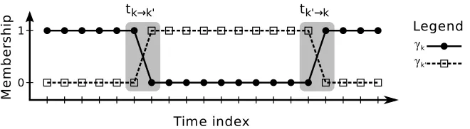
Figure 6: An example of the time-series data of membership signals. Transitions are highlighted in grey.

benefit is that sigmoid TM provides an elegant method to deal with uncertain or fuzzy memberships. Since the sigmoid is a continuous function ranging from 0 to 1, it is able to represent all degrees of membership as opposed to purely Boolean classification. The final benefit is inherited from SR: a range of solutions is provided via Pareto optimality, balancing model complexity and model accuracy, and model selection is used to prevent overfit solutions.

3.4 Modeling Hybrid Dynamical Systems

To infer symbolic models of hybrid dynamical systems, two general CSR and TM algorithms are applied to form the multi-modal symbolic regression algorithm (MMSR). CSR is first used to cluster the data into distinct modes while simultaneously inferring symbolic expressions for each subfunc-tion. Using the modal membership from CSR, TM is subsequently applied to find symbolic expres-sions for the transition conditions. Of the 4-tuple description of in Section 2.2,

H

= (

W

,

M

,

F

,

T

), the communication space,

W

, is provided by the time-series data and it is the goal of MMSR to determine the modes,

M

, behaviors,

F

, and transitions,

T

.

Using the unlabeled time-series data, the first step is to apply CSR. CSR determines the modes of the hybrid system,

M

, by calculating the membership of an input-output pair (expectation step of Algorithm 2). Simultaneously, CSR also infers a non-linear, symbolic expression for each of the behaviors,

F

, through weighted symbolic regression (maximization step of Algorithm 2).

Using the modal memberships from CSR, TM searches for symbolic expressions of the tran-sition events,

T

. To find the transitions, the data must be appropriately pre-processed within the hybrid system framework. Transition events are defined as the conditions for which the system moves from one mode to another. Using the membership values from CSR to determine the mode at every data point, searching for transition events is rephrased as a classification problem: a transi-tion from modekto modek′occurs at indexnif and only ifγk,n=1 andγk′_,n+1=1 (Figure 6). Thus, the classification problem is applied to membership levels of the origin and destination modes. For finding all transition events from modekto modek′, the search relationship and fitness metric are respectively:

γk′_,n+1=sig(t_k→k′(u_n)), Ftransition=−

N−1

∑

n=1

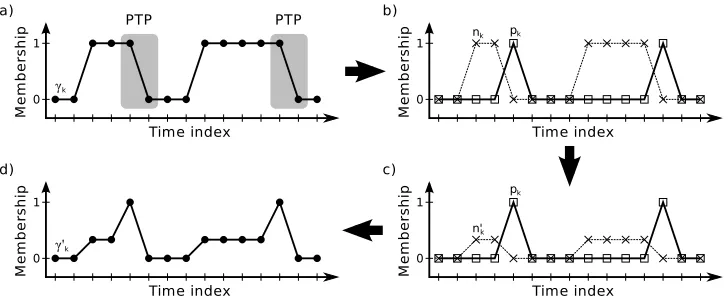
Figure 7: An example of PTP-NTP weight balance. a) Original weight data (γk,n). b) Weight data

decomposed intopk,nandnk,nsignals. c) Scaled ˜nk,nsignal. d)pk,n and ˜nk,nrecombined

to form balanced (˜γk,n).

It is important to realize that most data sets are heavily biased against observing transitions—the frequency at which a transition event occurs, or a positive transition point (PTP), is relatively rare compared to the frequency of staying in the same node, or negative transition point (NTP). A PTP is defined mathematically for modekat indexnifγk,n=1 andγk,n+1=0; all other binary

combi-nations of values are considered NTPs. This definition is advantageous since PTPs are identified by only using the membership information of only the current mode,γk,n, and no other membership

information from the other modes are required.

The relative frequencies of PTP and NTP affects the TM algorithm since the data set is imbal-anced: the sum of the weights associated with NTPs is significantly larger than the respective sum for PTPs. As a consequence, expressions which predict that no transitions ever occur result in a high fitness. Instead, equal emphasis on PTPs and NTPs via a simple pre-processor heuristic was found to provide much better learning for TM.

The first step in this weight rebalance pre-processing is to generate two new time-series signals, pk,nandnk,n, which decomposes the membership data into PTP and NTP components, respectively

(Equation 13-14). Thenk,nsignal is then scaled down by the ratio of the sum of the two components

(Equation 15), which ensures that the ˜nk,n signal has equal influence on TM as the pk,n signal.

Finally, the components are recombined to produced the new weights, ˜γk,n (Equation 16). This

process is illustrated in Figure 7.

pk,n=γk,n(1−γk,n+1), (13)

nk,n=γk,n−pk,n, (14)

˜

nk,n=nk,n

∑N−_n=11pk,n ∑N−_n=11nk,n

, (15)

˜

γk,n=pk,n+n˜k,n. (16)

all transition events from modekto modek′. The best expression is selected using the AIC ranking based on the transition fitness.

γk′_,n+1=sig(t_k→k′(u_n)), (17) Ftransition=−

∑N−_n=11˜γk,n||γk′_,n+1−sig(t_k→k′(u_n))||2

∑N−_n=11γ˜k,n

. (18)

The complete MMSR algorithm to learn analytic models of hybrid dynamical systems is sum-marized in Algorithm 3.

4. Results

This section begins with a description of the experimental setup for both the synthetic and real data experiments. Next is a discussion of the synthetic experiments, starting with an overview of alternative approaches, a list of the performance metrics, a summary of four data sets and finally, a discussion of MMSR performance in comparison to the baseline approaches. MMSR is then used to identify and characterize field-effect transistor modes, similar to those derived from first principles, based on real data. This section concludes with a brief discussion of the scalability of MMSR.

4.1 Experimental Details

In these experiments, the publicly available Eureqa API (Schmidt and Lipson, 2012) was used as a backend for the symbolic regression computation in both the CSR and TM. To illustrate the robustness of MMSR, the same learning parameters were applied across all the data sets, indicating that task-specific tuning of these parameters was not required:

• The SR for CSR was initially executed for 10000 generations and this upper limit was in-creased by 200 generations every iteration, until the global error produced less than 2% change for five EM iterations. Once CSR was complete, the SR for TM was a single 20000 generation search for each transition.

• The CSR algorithm was provided all the continuous inputs, while the TM algorithm was also provided with the one-hot encoding of binary signals, according to the data.

• The default settings in Eureqa, the SR backend, were used:

– Population size = 64

– Mutation probability = 3%

– Crossover probability = 70%

Algorithm 3Multi-modal Symbolic Regression

input → unclustered input-output data - un,yn → the number of subfunctions - K

output → behavior for each mode - fk(un) → variance for each mode - σ2

k

→ transitions between each mode - tk→k′(un)

function symbolic_regression(search_relationship, fitness_function) :

initialize population with random expressions defined by search_relationship for predefined computational effort :

generate new expressions from existing population (Figure 4) calculate fitness of all expressions according to fitness_function remove unsuitable expressions from the population

for each pop_expr in the population : for each pareto_expr in the pareto_set :

if ((pop_expr.fitness > pareto_expr.fitness) and (pop_expr.complexity <= pareto_expr.complexity)) : add pop_expression to pareto_set

remove pareto_expression from pareto set return pareto_set

# Clustered symbolic regression initialize random membership values for each behavior in K modes :

sr_solutions = symbolic_regression(Equation 6, Equation 7)

set behavior fk to solution with lowest local AIC score in sr_solutions set variance for each behavior - σ2

k (Equation 5) while convergence is not achieved :

for each behavior in K modes : # expectation step

for all the N data points :

compute membership values - γk,n (Equation 4) # maximization step

sr_solutions = symbolic_regression(Equation 6, Equation 7) for each solution in sr_solutions :

compute temporary membership values - γˇk,n (Equation 4) compute temporary variance - σˇ2

k (Equation 5)

compute global fitness using temporary values - ECSR (Equation 2) compute AIC score using global fitness (Equation 8)

set behavior fk to solution with lowest AIC score in sr_solutions set variance to corresponding value - σ2

k (Equation 5) # Transition modelling

for each mode k in K modes :

for each different mode k′ in K−1 modes :

rebalance the PTP and NTP weights (Equation 13-16)

tm_solutions = symbolic_regression(Equation 17, Equation 18) for each solution in tm_solutions :

compute AIC score using transition fitness (Equation 8)

set transition tk→k′(un) to solution with lowest AIC score in tm_solutions

Figure 8: Schematic diagram of the fully recurrent neural network.

4.2 Synthetic Data Experiments

This section discusses a collection of experiments on hybrid systems generated by computer simula-tion. It begins with an introduction of alternative multi-modal model inference approaches, followed by an outline of the metrics used to measure their performance and a description of the data sets used for model comparison. This section concludes with a summary and discussion of the experimental results.

4.2.1 ALTERNATIVEMODELS

This subsection describes two traditional machine learning approaches to modeling multi-modal time-series data: fully recurrent neural networks and neural network based, input-output hidden Markov machines.

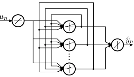
Fully Recurrent Neural Network—A fully recurrent neural network (RNN) is a neural network where connections form a directed cycle (Figure 8). This baseline recurrent network was composed of an input layer of nodes with linear transfer functions, a single hidden layer of nodes with sig-moidal transfer functions and a linear transfer function as the output node. The output of the hidden layer was consequently fed back as an input with a one cycle delay, allowing the network to store memory and making it capable of modelling multi-modal behavior.

The network was implemented using the open source, machine learning library PyBrain (Schaul et al., 2010) and was trained via backpropagation through time (Rumelhart et al., 1986). The training data was split into a training and validation subset, where the training subset consists of the initial contiguous 75% portion of the data. The training was terminated either via early stopping or when the training error decreased by less than 0.01% for 10 iterations. The size of the hidden layers, h, ranged from 10, 25, 50 to 100 nodes based on complexity of the data set. The weights were initialized by sampling a zero mean Gaussian random variable with a standard deviation of 1. The learning rate was ε=0.0005/hand used a momentum of 0.1. The learning rate was sufficiently small that the gradients never grew exponentially.

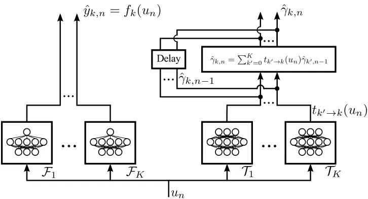
input-Figure 9: Schematic diagram of the neural network based IOHMM architecture (Bengio and Fras-coni, 1994).

F

_k are regression networks with a single sigmoidal hidden layer and

T

_k are softmax networks with a single sigmoidal hidden layer.

output networks used linear input and output layers while the state prediction network used a linear input layer and a softmax output layer.

The generalized EM algorithm (GEM) was applied for training was terminated either via early stopping or when the validation error produced less than a 0.01% decrease for 50 EM iterations. The size of the hidden layers,h, are identical for every network in the architecture and ranged from 5, 10, and 20 nodes. The weights were initialized by sampling a zero mean Gaussian random variable with a standard deviation of 1. The learning rate was ε=0.0002/h with no momentum. The learning rate was sufficiently small that the gradients never grew exponentially.

4.2.2 PERFORMANCEMETRICS

There are three performance metrics of interest: model accuracy, complexity and fidelity.

Model accuracyis a measure of ability of a learning algorithm to predict outputs given inputs.

The trained model is used to predict the evolution of the time series data and the error is the negative log probability of a mixture of Laplacians (Equation 1).

For time series prediction, the accumulation of the state error over time, also known as drift, becomes a significant factor. Repeated iterations of accurate but not-perfect transitions over a prolonged period of time will result in a significant accumulated error. Drift is managed with a closed-loop system (Figure 10), where the output of the previous time step is also provided. With the MMSR algorithm, a closed-loop model is trivially constructed by setting the previous state probabilities according to the clustering component in CSR. However, the neural network based algorithms cannot be reformed into a closed-loop model without retraining the network or adapting the framework to execute some form of clustering.

Model complexity is a measure of the total number of free parameters required for the model.

Figure 10: Schematic diagram of an open-loop and closed-loop system in a) and b), respectively.

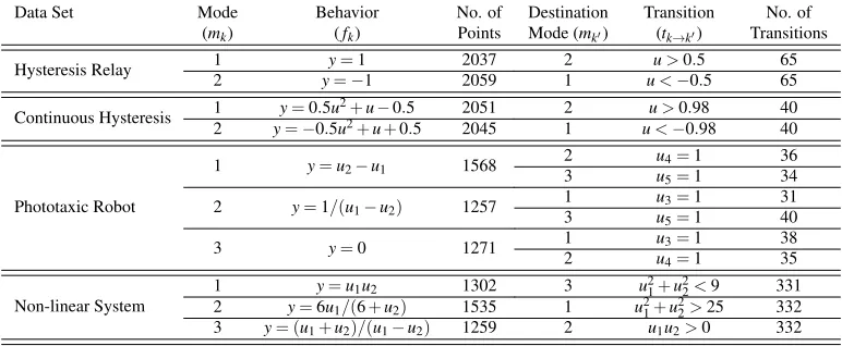
Data Set Mode Behavior No. of Destination Transition No. of (mk) (fk) Points Mode (mk′) (tk→k′) Transitions

Hysteresis Relay 1 y=1 2037 2 u>0.5 65

2 y=−1 2059 1 u<−0.5 65

Continuous Hysteresis 1 y=0.5u

2_{+u−0.5 2051 2 u>0.98 40}

2 y=−0.5u2+u+0.5 2045 1 u<−0.98 40

Phototaxic Robot

1 y=u2−u1 1568 ₃2 u_u4=1 36

5=1 34

2 y=1/(u1−u2) 1257 1 u3=1 31

3 u5=1 40

3 y=0 1271 1 u3=1 38

2 u4=1 35

Non-linear System

1 y=u1u2 1302 3 u21+u22<9 331

2 y=6u1/(6+u2) 1535 1 u21+u22>25 332

3 y= (u1+u2)/(u1−u2) 1259 2 u1u2>0 332 Table 1: Summary of test data sets

The neural network based algorithms have a static complexity, which is the number of hidden nodes in all of subnetworks. Although the node count does not account for the complexity of operations and more comprehensive measures exist (Vladislavleva et al., 2009), it does provide a simple and coarse measure of complexity and acts as a first approximation to human interpretability.

Model fidelityis a measure of the MMSR’s ability to reproduce the form or mathematical

struc-ture of original system. This metric is important as it integral to the primary goal of knowledge extraction—predictive accuracy is insufficient as the models must reproduce the expressions and not an approximation.

In symbolic representations, expressions are considered equivalent if and only if each subtree differs by at most scalar multiplicatives. For example, the expressiony=u2/(1+u)is considered to be equivalent to y=1.1u2/(0.9+u), but the Taylor series approximation about u=1→y=

−0.125+0.5u+0.125u2 is considered dissimilar regardless of its numeric accuracy. The fidelity is measured as the percentage of correctly inferred expression forms. In comparison, all neural network based systems are function approximations by design and thus, are immeasurable with respect to model fidelity.

4.2.3 DATASETS

Data Set Name System Diagram Data Plot

Hysteresis Relay

−2 −1 0 1 2 −1.5

−1 −0.5 0 0.5 1 1.5

u

y

Continuous Hysteresis Loop

−1 −0.5 0 0.5 1 −1

−0.5 0 0.5 1

u

y

Phototaxic Robot

−6 −4 −2 0 2 4 6 −6

−3 0 3 6

u

1 − u2

y

Non-linear System

−5 0 5 −5 0 5 −30

−15 0 15 30

u

1

u

2

y

Figure 11: The system diagram and plots of the noiseless test data sets.

These data sets range in complexity in both the discrete and continuous domains. Furthermore, these data sets contain non-trivial transitions and behaviors, and thus, present more challenging in-ference problems than the simple switching systems often used to evaluate parametric models of hybrid systems (Le et al., 2011). Simple switching systems have trivial discrete dynamics where the transition to any mode does not depend on the current mode.

Training and test sets were generated; the training sets were corrupted with varying levels of additive Gaussian noise, while the test sets remained noiseless. The level of noise was defined as the ratio of the Gaussian standard deviation to the standard deviation of the data set (Equation 19). The noise was varied from 0% to 10% in 2% increments.

Np=

σnoise σy

. (19)

The statistics of all four data sets are summarized in Table 1, while the system diagrams and test data set are shown in Figure 11.

linear behaviors, it does not exhibit simple switching as the transitions depend on the mode since both behaviors are defined foru∈[−0.5,0.5].

Continuous Hysteresis Loop—The second data set is a continuous hysteresis loop: a non-linear extension of the classical hybrid system (Visintin, 1995). The Preisach model of hysteresis is used, where numerous hysteresis relays are connected in parallel and summed. As the number of hystere-sis relays approaches infinity, a continuous loop is achieved. The data set is generated by repeatedly completing a single pass in the loop. Although there are still two modes, this data set is significantly more complex due to the symmetry of error functions about the liney=u, as well as the fact that transition depend on the mode and occur at a continuity in the output domain.

Phototaxic Robot—The third data set is a light-interacting robot (Reger et al., 2000). The robot has phototaxic movement: it either approaches, avoids, or remains stationary depending on the color of light. The outputyis velocity of the robot. There are five inputs:u1andu2are the absolute

positions of robot and light, respectively, while {u3,u4,u5} is a binary, one-hot encoding of the

light color, where 0 indicates the light is off and 1 indicates the light is on. This modeling problem is challenging due to the variety of inputs and non-uniform distribution of data. However, it does exhibit simple modal switching behavior that only depends on the light input.

Non-linear System—The fourth and final data set is a system without any physical counterpart, but the motivation for this system was to evaluate the capabilities of the learning algorithms for finding non-linear, symbolic expressions. The system consists of three modes, where all of the behaviors and transition conditions consist of non-linear equations which cannot be modeled via parametric regression without incorporating prior knowledge. All the expressions are a function of the variablesu1andu2, the discriminant functions are not linearly separable and the transitions are

modally dependent.

4.2.4 EXPERIMENTALRESULTS

MMSR, along with the two parametric baselines, was evaluated on all four data sets and the perfor-mance metrics are summarized in Figure 12. This section begins with overview of the algorithms’ general performance, followed by case study analysis of each data set in the following subsections.

First, MMSR was able to reliably reconstruct the original model from the unlabeled, time-series data. The process of converting the program output into a hybrid automata model is summarized in Figure 13, from a run obtained on the light-interacting robot training data with 10% noise. Provided with the number of modes, the algorithm searched for distinct behaviors and their subsequent transi-tions, returning a single symbolic expression for each of the inferred components. The expressions were algebraically simplified as necessary, and a hybrid dynamical model was constructed.

Comparing the algorithms on predictive accuracy, the closed-loop MMSR model outperformed the neural network baselines on every data set across all the noise conditions. The open-loop MMSR model was able to achieve similar performance to its closed-loop counterpart for most systems, with the exception of the noisy continuous hysteresis loop. For low noise conditions, MMSR achieves almost perfect predictions, even in open-loop configurations.

Model Accuracy Model Complexity Model Fidelity L eg en d H y ste re sis R ela y

0 2 4 6 8 10 0

0.05 0.1 0.15 0.2

Predictive Error (E)

Noise (N

p)

0 20 40 60 80 100 0

0.05 0.1 0.15 0.2

Predictive Error (E)

Complexity

0 2 4 6 8 10 0 0.2 0.4 0.6 0.8 1 Convergence Probability Noise (N p) C o n tin u o u s H y ste re sis L o o p

0 2 4 6 8 10 0

0.05 0.1 0.15 0.2

Predictive Error (E)

Noise (N

p)

0 20 40 60 80 100 0

0.05 0.1 0.15 0.2

Predictive Error (E)

Complexity

0 2 4 6 8 10 0 0.2 0.4 0.6 0.8 1 Convergence Probability Noise (N p) P h o to ta x ic R o b o t

0 2 4 6 8 10 0 0.1 0.2 0.3 0.4 0.5

Predictive Error (E)

Noise (N

p)

0 100 200 300 0 0.1 0.2 0.3 0.4 0.5

Predictive Error (E)

Complexity

0 2 4 6 8 10 0 0.2 0.4 0.6 0.8 1 Convergence Probability Noise (N p) N o n -lin ea r S y ste m

0 2 4 6 8 10 0

0.2 0.4 0.6

Predictive Error (E)

Noise (N

p)

0 100 200 300 0

0.2 0.4 0.6

Predictive Error (E)

Complexity

0 2 4 6 8 10 0 0.2 0.4 0.6 0.8 1 Convergence Probability Noise (N p)

Figure 12: The performance metrics on four systems. Error bars indicate standard error (n=10).

However, other than the simplest data set, none of the parametric approaches were able to converge on an accurate representation, even with noiseless training data.

//Behaviors f1(u)=0.0017 f2(u)=0.996/(u1-u2) f3(u)=u2-u1

//Transitions

f1->f2=sig(11.87*u4-7.60)

f1->f3=sig(128.0*u1ˆ2*u3-30.72*u1ˆ2) f2->f1=sig(16.11*u2ˆ2*u5-12.35*u2ˆ2) f2->f3=sig(45.09*u2ˆ2*u3-9.47*u2ˆ2) f3->f1=sig(174.9*u4-73.49)

f3->f2=sig(9.28*u1ˆ2*u5-5.38*u1ˆ2)

(a) Program Output (b) Inferred System Diagram

−6 −4 −2 0 2 4 6

−6 −4 −2 0 2 4 6

u₁−u₂

y

(c) Behaviors with Training Data

Figure 13: Conversion from program output to hybrid dynamical model for the phototaxic robot with 10% noise. Algebraic simplifications were required to convert program output (a) to inequalities in canonical form (c).

Furthermore, not only was MMSR a superior predictor, the numerical accuracy was achieved with less free parameters than the neural network baselines. Even though the measure of counting nodes provides only a coarse measure of complexity, the neural network approaches have signifi-cantly more error despite having up to five times the number of free parameters on noiseless training data. This suggests that the symbolic approach is better suited for the primary goal of knowledge extraction, by providing accurate as well as parsimonious models.

In addition, for the neural network approaches, increasing the model complexity does not nec-essarily result in greater accuracy. In fact, for most data sets, once the number of hidden nodes reached a threshold, the trained models generally become less accurate despite having additional modelling capabilities. For multi-model problems, the parameter space is non-convex and contains local optima—as the number of hidden nodes increases, the probability of finding a local optima increases as well. Thus, for parametric models, the number of hidden nodes must be tuned to ac-count for the complexity of the data set, presenting another challenge to the arbitrary application of parametric models.

Finally, MMSR was able to achieve reliable model fidelity. In the noiseless training sets, the correct expressions for both the behaviors and events were inferred with perfect reliability. As the signal to noise ratio was increased, the probability of convergence varied significantly depending on the characteristics of the data set. Generally, the algorithm was able to repeatedly find the correct form for the behaviors for the majority of the data sets. In contrast, the transition expressions were more difficult to infer since the model fidelity deteriorates at lower noise levels. This is a result of TM’s dependence on accurate membership values from CSR—noisy data leads to larger classification errors, amplifying the challenge of modeling transitions.

Despite the model fidelity’s sensitivity to noise, the algorithm was nonetheless able to accurately predict outputs for a wide range of noise conditions. The inferred expressions, regardless of the expression fidelity, were still accurate numerical approximations for both open- and closed-loop models.

−1 −0.5 0 0.5 1 −1

−0.5 0 0.5 1

u

y

NNHMM with lowest error

(a)

−1 −0.5 0 0.5 1

−1 −0.5 0 0.5 1

u

y

NNHMM with greatest separation

(b)

−1 −0.5 0 0.5 1

−1 −0.5 0 0.5 1

u

y

MMSR with lowest error

(c)

Figure 14: The input-output relationship of the regression networks of NNHMM and symbolic ex-pressions of MMSR (black) overlaid on the Continuous Hysteresis Loop data (grey).

near perfect accuracy with ten or more hidden nodes per network, but failed when provided with only five hidden nodes per network. In terms of model fidelity, MMSR was able to achieve perfect expressions with respect to all the noise conditions.

Continuous Hysteresis Loop—This data set was ideal as it was sufficiently difficult to model, but simple enough to analyze and provide insight into how the algorithms perform on hybrid dynamical systems. The closed-loop MMSR was able to significantly outperform NNHMM and RNN under all noise conditions, but the open-loop MMSR fared worse than the parametric baselines in the presence of noise. This result was particularly interesting, since perfect model fidelity was achieved for all noise conditions. The predictive error in the open-loop MMSR occurred as a result of the continuous transition condition—under noisy conditions, the model can fail to predict a transition even with a correct model. As a result, a missed transition accumulates significant error for open-loop models. A closed-open-loop model is able to account for missed transitions, resulting in consistently accurate models.

Next, NNHMM outputs were analyzed to understand the discrepancy in predictive accuracy. Figure 14 shows the input-output relationships of NNHMM’s best performing model, NNHMM’s model that obtains the greatest separation and MMSR’s best performing model, respectively. NNHMM had significant difficulties breaking the symmetry in the data set as the best model cap-tured only the symmetry, while the locally-optimal asymmetrical model was both inferior in predic-tive accuracy and was significantly far from the ground truth. In comparison, MMSR was able to deal with the symmetrical data and infer unique representations. Such analysis could not be applied to RNNs as it is impossible to decouple the input-output relationships from the model transition components.

(a) Circuit Diagram

0 1

2 3

4 5

0 1 2 3 4 5 0 0.2 0.4 0.6 0.8 1

Gate Voltage (vGS) [V] Drain Voltage (vDS) [V]

Drain Current (i

D

) [A]

(b) Measured Data

Figure 15: A circuit diagram indicating the two input voltages,vGSandvDS, and the output current

iD, and the measured 3D data plot from the ZVNL4206AV nMOSFET.

This data set provides an example of how symbolic expressions aid in knowledge abstraction as it is easy to infer that the relative distance between the robot and the light position, u1−u2, is

an integral component of the system as it is a repeated motif in the each of the behaviors. It is significantly more difficult to extract the same information from parametric approaches like neural networks.

Non-linear System—The final data set provided a difficult modelling challenge that included non-linear behaviors which cannot be modeled by by parametric regression. Yet, MMSR reliably inferred the correct model for low noise systems and produced accurate predictions in all noise levels despite the noise sensitivity of model fidelity. The neural network approaches were significantly less accurate while using more free parameters.

4.3 Real Data Experiment

This section provides a case study of MMSR on real-world data while also exemplifying the benefits of symbolic model inference. This case study involves the inference of an n-channel metal-oxide semiconductor field-effect transistor (nMOSFET), a popular type of transistor ubiquitous in digital and analog circuits. nMOSFETs exhibit three distinct characteristics, which are governed by the physical layout and the underlying physics (Sedra and Smith, 2004), making them an ideal candidate for hybrid system analysis.

The transistor was placed in a standard configuration to measure the current-voltage character-istics, where the drain current is set as a function of the gate and drain voltages (Figure 15a). The transistor was a Diodes Inc. ZVNL4206AV nMOSFET and the data was recorded with a Keithley 2400 general purpose sourcemeter. The data was collected via random voltage sweeps from 0-5V, and the subsequent current was measured (Figure 15b).

(a) Inferred system diagram

iD=

( _{4.29e-8 , ifv}

GS≤2.02

0.46 (vGS−2.59)vDS−0.71v2DS

, ifvGS>2.68 and(vGS−1.01vDS)>2.39

0.17(vGS−2.76)(VGS−2.40) , ifvGS>2.11 and(vGS−0.98vDS)≤2.43 (b) Inferred mode expressions

iD=

 



0 , ifvGS≤k1

k2 (vGS−k1)vDS−1₂v2DS

, ifvGS>k1and(vGS−vDS)>k1 1

2k2(vGS−k1)2 , ifvGS>k1and(vGS−vDS)≤k1

(c) Classically derived mode expressions

Figure 16: The inferred hybrid model compared to the derived expressions.

was applied for ten independent runs and the median performing model was reported. As the tran-sitions events were consistent between modes, which is indicative of the simple switching behavior exhibited by transistors, the system diagram was simplified to a piecewise representation with addi-tional symbolic manipulations (Figure 16b).

When the inferred expressions are compared to classical equations (Sedra and Smith, 2004), the results are remarkably similar (Figure 16c). This suggests that MMSR is capable of inferring the ground truth of non-trivial systems from real-world data. While the model is sufficiently nu-merically accurate, the more impressive and relevant consequence is that MMSR was able to find the same expressions as engineer would derive from first principles, but inferred the results from unlabeled data. For an engineer or scientist presented with an unknown device with multi-modal behavior, beginning with apt, mathematical descriptions of a system might provide essential insight and understanding to determining the governing principles of that system. This capability provides an important advantage over traditional parametric machine learning models.

4.4 Scalability

than a traditional lower-bound analysis, analyzing the computational complexity is used to provide insight to the scope of problems that are well suited for MMSR inference.

To assess the performance scalability of MMSR, the computational complexity of SR must first be analyzed as it is the primary computational kernel. As convergence on the global solution is not guaranteed, in the worst-case analysis, the complete search space is exhausted in a stochastic manner. Forbbuilding blocks and a tree depth size ofcnodes, the search space grows exponentially with a complexity ofO(bc). However, on average, SR performs significantly better than the worst case, although the performance is highly case dependent. Furthermore, evolutionary algorithms are naturally parallel, providing scalability with respect to the number of processors.

For the MMSR learning algorithm, two components are analyzed independently. With the worst-case SR complexity O(bc) and k modes, CSR has a compounded linear complexity with respect to the number of modes,O(kbc_{), while TM has a quadratic complexity ofO(k}2_bc_{), since}

transitions for every combination of modes must be considered. In terms of worst-case computa-tional effort, this suggests that this algorithm would scale better for systems with numerous simple modes than it would for systems with fewer modes of higher complexity. For the data sets described in this section, the algorithm required an average of 10 and 45 minutes for the bi- and tri-modal sys-tems, respectively, on a single core of a 2.8GHz Intel processor.

5. Discussion and Future Work

A novel algorithm, multi-modal symbolic regression (MMSR), was presented to infer non-linear, symbolic models of hybrid dynamical systems. MMSR is composed of two general subalgorithms. The first subalgorithm is clustered symbolic regression (CSR), designed to construct expressions for piecewise functions of unlabeled data. By combining symbolic regression (SR) with expectation-maximization (EM), CSR is able to separate the data into distinct clusters, and then subsequently find mathematical expressions for each subfunction. CSR exploits the Pareto front of SR to con-sistently avoid locally optimal solutions, a common challenge in EM mixture models. The second subalgorithm is transition modeling (TM), which searches for binary classification boundaries and expresses them as a symbolic inequality. TM uniquely capitalizes on the pre-existing SR infras-tructure through function composition. These two subalgorithms are combined and used to infer symbolic models of hybrid dynamical systems.

MMSR is applied to four synthetic data sets, which span a range of classical hybrid automata and intelligent robotics. The training data was also corrupted with various levels of noise. The inferred models were compared via three performance metrics: model accuracy, complexity, and fidelity. MMSR inferred reliable models for noiseless data sets and outperformed its neural network counterparts in both model accuracy as well as model complexity. Furthermore, MMSR was used to identify and characterize field-effect transistor modes, similar to those derived from first principles, demonstrating a possible real-world application unique to this algorithm.