Efficient Structure Learning of Bayesian Networks using Constraints

Efficient Structure Learning of Bayesian Networks using Constraints

Cassio P. de Campos [email protected]

Dalle Molle Institute for Artificial Intelligence Galleria 2

Manno 6928, Switzerland

Qiang Ji [email protected]

Dept. of Electrical, Computer & Systems Engineering Rensselaer Polytechnic Institute

110 8th Street Troy, NY 12180, USA

Editor: David Maxwell Chickering

Abstract

This paper addresses the problem of learning Bayesian network structures from data based on score functions that are decomposable. It describes properties that strongly reduce the time and memory costs of many known methods without losing global optimality guarantees. These properties are derived for different score criteria such as Minimum Description Length (or Bayesian Information Criterion), Akaike Information Criterion and Bayesian Dirichlet Criterion. Then a branch-and-bound algorithm is presented that integrates structural constraints with data in a way to guarantee global optimality. As an example, structural constraints are used to map the problem of structure learning in Dynamic Bayesian networks into a corresponding augmented Bayesian network. Fi-nally, we show empirically the benefits of using the properties with state-of-the-art methods and with the new algorithm, which is able to handle larger data sets than before.

Keywords: Bayesian networks, structure learning, properties of decomposable scores, structural constraints, branch-and-bound technique

1. Introduction

A Bayesian network is a probabilistic graphical model that relies on a structured dependency among random variables to represent a joint probability distribution in a compact and efficient manner. It is composed by a directed acyclic graph (DAG) where nodes are associated to random variables and conditional probability distributions are defined for variables given their parents in the graph. Learning the graph (or structure) of these networks from data is one of the most challenging prob-lems, even if data are complete. The problem is known to be NP-hard (Chickering et al., 2003), and best exact known methods take exponential time on the number of variables and are applicable to small settings (around 30 variables). Approximate procedures can handle larger networks, but usually they get stuck in local maxima. Nevertheless, the quality of the structure plays a crucial role in the accuracy of the model. If the dependency among variables is not properly learned, the estimated distribution may be far from the correct one.

re-search on this topic is active (Chickering, 2002; Teyssier and Koller, 2005; Tsamardinos et al., 2006; Silander and Myllymaki, 2006; Parviainen and Koivisto, 2009; de Campos et al., 2009; Jaakkola et al., 2010), mostly focused on complete data. In this case, best exact ideas (where it is guaran-teed to find the global best scoring structure) are based on dynamic programming (Koivisto and Sood, 2004; Singh and Moore, 2005; Koivisto, 2006; Silander and Myllymaki, 2006; Parviainen and Koivisto, 2009), and they spend time and memory proportional to n·2n, where n is the number of variables. Such complexity forbids the use of those methods to a couple of tens of variables, mainly because of the memory consumption (even though time complexity is also a clear issue). Ott and Miyano (2003) devise a faster algorithm when the complexity of the structure is limited (for instance the maximum number of parents per node and the degree of connectivity of a subja-cent graph). Perrier et al. (2008) use structural constraints (creating an undirected super-structure from which the undirected subjacent graph of the optimal structure must be a subgraph) to reduce the search space, showing that such direction is promising when one wants to learn structures of large data sets. Kojima et al. (2010) extend the same ideas by using new search strategies that exploit clusters of variables and ancestral constraints. Most methods are based on improving the dynamic programming method to work over reduced search spaces. On a different front, Jaakkola et al. (2010) apply a linear programming relaxation to solve the problem, together with a branch-and-bound search. Branch-branch-and-bound methods can be effective when good bounds and cuts are available. For example, this has happened with certain success in the Traveling Salesman Problem (Applegate et al., 2006). We have proposed an algorithm that also uses branch and bound, but em-ploys a different technique to find bounds (de Campos et al., 2009). It has been showed that branch and bound methods can handle somewhat larger networks than the dynamic programming ideas. The method is described in detail in Section 5.

In the first part of this paper, we present structural constraints as a way to reduce the search space. We explore the use of constraints to devise methods to learn specialized versions of Bayesian networks (such as naive Bayes and Tree-augmented naive Bayes) and generalized versions, such as Dynamic Bayesian networks (DBNs). DBNs are used to model temporal processes. We describe a procedure to map the structural learning problem of a DBN into a corresponding augmented Bayesian network through the use of further constraints, so that the same exact algorithm we discuss for Bayesian networks can be employed for DBNs.

In the second part, we present some properties of the problem that bring a considerable improve-ment on many known methods. We build on our recent work (de Campos et al., 2009) on Akaike Information Criterion (AIC) and Bayesian Information Criterion (BIC), and present new results for the Bayesian Dirichlet (BD) criterion (Cooper and Herskovits, 1992) and some derivations under a few assumptions. We show that the search space of possible structures can be reduced drastically without losing the global optimality guarantee and that the memory requirements are very small in many practical cases.

pre-computed during an initialization step to save computational time. Then we perform the search over the possible graphs iterating over arcs. Because of the B&B properties, the algorithm can be stopped with a best current solution and an upper bound for the global optimum, which gives a certificate to the answer and allows the user to stop the computation when she/he believes that the current solution is good enough. For example, such an algorithm can be integrated with a structural Expectation-Maximization (EM) method without the huge computational expenses of other exact methods by using the generalized EM (where finding an improving solution is enough), but still guaranteeing that a global optimum is found if run until the end. Due to this property, the only source of approximation would regard the EM method itself. It worth noting that using a B&B method is not new for structure learning (Suzuki, 1996). Still, that previous idea does not constitute a global exact algorithm, instead the search is conducted after a node ordering is fixed. Our method does not rely on a predefined ordering and finds a global optimum structure considering all possible orderings.

The paper is divided as follows. Section 2 describes the notation and introduces Bayesian net-works and the structure learning problem based on score functions. Section 3 presents the structural constraints that are treated in this work, and shows examples on how they can be used to learn dif-ferent types of networks. Section 4 presents important properties of the score functions that consid-erably reduce the memory and time costs of many methods. Section 5 details our branch-and-bound algorithm, while Section 6 shows experimental evaluations of the properties, the constraints and the exact method. Finally, Section 7 concludes the paper.

2. Bayesian Networks

A Bayesian network represents a joint probability distribution over a collection of random variables, which we assume to be categorical. It can be defined as a triple(

G

,

X

,

P

), where

G

= (. VG,EG)is a directed acyclic graph (DAG) with VG a collection of n nodes associated to random variables

X

(a node per variable), and EG a collection of arcs;

P

is a collection of conditional mass functions p(Xi|Πi)(one for each instantiation ofΠi), whereΠidenotes the parents of Xiin the graph (Πimay

be empty), respecting the relations of EG. In a Bayesian network every variable is conditionally independent of its non-descendants given its parents (Markov condition).

We use uppercase letters such as Xi,Xj to represent variables (or nodes of the graph, which

are used interchanged), and xi to represent a generic state of Xi, which has state space ΩXi

.

= {xi1,xi2, . . . ,xiri}, where ri

.

=|ΩXi| ≥2 is the number of (finite) categories of Xi (| · |is the cardi-nality of a set or vector, and the notation=. is used to indicate a definition instead of a mathematical equality). Bold letters are used to emphasize sets or vectors. For example, x∈ΩX=. ×X∈XΩX,

for X⊆

X

, is an instantiation for all the variables in X. Furthermore, rΠi

.

=|ΩΠi|=∏Xt∈Πirt is the number of possible instantiations of the parent setΠi of Xi, andθ= (θi jk)∀i jkis the entire

vec-tor of parameters such that the elements areθi jk=p(xik|πi j), with i∈ {1, . . . ,n}, j∈ {1, ...,rΠi}, k∈ {1, ...,ri}, andπi j∈ΩΠi.

Because of the Markov condition, the Bayesian network represents a joint probability distribu-tion by the expression p(x) =p(x1, . . . ,xn) =∏ip(xi|πi), for every x∈ΩX, where every xi andπi

are consistent with x.

nodes

X

, for a given score function sD(the dependency on data is indicated by the subscript D).1In

this paper, we consider some well-known score functions: the Bayesian Information Criterion (BIC) (Schwarz, 1978) (which is equivalent to the Minimum Description Length), the Akaike Information Criterion (AIC) (Akaike, 1974), and the Bayesian Dirichlet (BD) (Cooper and Herskovits, 1992), which has as subcases BDe and BDeu (Buntine, 1991; Cooper and Herskovits, 1992; Heckerman et al., 1995). As done before in the literature, we assume parameter independence and modularity (Heckerman et al., 1995). The score functions based on BIC and AIC differ only in the weight that is given to the penalty term:

BIC/AIC : sD(

G

) =max

θ LG,D(θ)−t(

G

)·w,

where t(

G

) =∑n_i=1(rΠi·(ri−1))is the number of free parameters, w= logN

2 for BIC and w=1 for AIC, LG,Dis the log-likelihood function with respect to data D and graph

G

:

LG,D(θ) =log n

∏

i=1

rΠi

∏

j=1

ri

∏

k=1

θni jk

i jk,

where ni jkindicates how many elements of D contain both xikandπi j. Note that the values(ni jk)∀i jk

depend on the graph

G

(more specifically, they depend on the parent setΠi of each Xi), so a more

precise notation would be to use nΠi

i jkinstead of ni jk. We avoid this heavy notation for simplicity

un-less necessary in the context. Moreover, we know thatθ∗= (θ∗_{i jk})∀i jk= ( ni jk

ni j )∀i jk=argmaxθLG,D(θ), with ni j=∑kni jk.2

In the case of the BD criterion, the idea is to compute a score based on the posterior probability of the structure p(

G

|D). For that purpose, the following score function is used:

BD : sD(

G

) =log

p(

G

)·

Z

p(D|

G

,θ)·p(θ|

G

)dθ

,

where the logarithmic is often used to simplify computations, p(θ|

G

)is the prior ofθfor a given graph

G

, assumed to be a Dirichlet with hyper-parametersα= (αi jk)∀i jk(which are assumed to be

strictly positive):

p(θ|

G

) =

n

∏

i=1

rΠi

∏

j=1

Γ(αi j) ri

∏

k=1

θαi jk−1

i jk

Γ(αi jk)

,

whereαi j=∑kαi jk. Hyper-parameters(αi jk)∀i jkalso depend on the graph

G

, and we indicate it by

αΠi

i jk if necessary in the context. From now on, we also omit the subscript D. We assume that there

is no preference for any graph, so p(

G

) is uniform and vanishes in the computations. Under the assumptions, it has been shown (Cooper and Herskovits, 1992) that for multinomial distributions,

s(

G

) =log

n

∏

i=1

rΠi

∏

j=1

Γ(αi j)

Γ(αi j+ni j) ri

∏

k=1

Γ(αi jk+ni jk)

Γ(αi jk)

.

The BDe score (Heckerman et al., 1995) assumes thatαi jk=α∗·p(θi jk|

G

), whereα∗is the

hyper-parameter known as the Equivalent Sample Size (ESS), and p(θi jk|

G

)is the prior probability for 1. In case of many optimal DAGs, then we assume to have no preference and argmax returns one of them.

2. If ni j=0, then ni jk=0 and we assume the fraction

ni jk

(xik∧πi j)given

G

(or simply givenΠi). The BDeu score (Buntine, 1991; Cooper and Herskovits,

1992) assumes further that local priors are such that αi jk becomes α ∗

rΠiri and α

∗ _{is the only free}

hyper-parameter.

An important property of all such criteria is that their functions are decomposable and can be written in terms of the local nodes of the graph, that is, s(

G

) =∑n_i=1si(Πi), such that

BIC/AIC : si(Πi) =max

θi

L_Πi(θi)−ti(Πi)·w, (1)

where L_Πi(θi) =∑ rΠi

j=1∑

ri

k=1ni jklogθi jk, and ti(Πi) =rΠi·(ri−1). And similarly,

BD : si(Πi) = rΠi

∑

j=1

log Γ(αi j)

Γ(αi j+ni j)

+

ri

∑

k=1

logΓ(αi jk+ni jk)

Γ(αi jk) !

. (2)

In the case of BIC and AIC, Equation (1) is used to compute the global score of a graph using the local scores at each node, while Equation (2) is employed for BD, BDe and BDeu, using the respective hyper-parametersα.

3. Structural Constraints

A way to reduce the space of possible DAGs is to consider some constraints provided by experts. We work with structural constraints that specify where arcs may or may not be included. These constraints help to reduce the search space and are available in many situations. Moreover, we show examples in Sections 3.1 and 3.2 of how these constraints can be used to learn structures of different types of networks, such as naive Bayes, tree-augmented naive Bayes, and Dynamic Bayesian networks. We work with the following rules, used to build up the structural constraints:

• indegree(Xj,k,op), where op∈ {lt,eq}and k an integer, means that the node Xj must have

less than (when op=lt) or equal to (when op=eq) k parents.

• arc(Xi,Xj)indicates that the node Ximust be a parent of Xj.

• Operators or (∨) and not (¬) are used to form the rules. The and operator is not explicitly used as we assume that each constraint is in disjunctive normal form.

The structural constraints can be imposed locally as long as they involve just a single node and its parents. In essence, parent sets of a node Xi that do violate a constraint are never processed

3.1 Learning Naive and TAN structures

For example, the constraints ∀i6=c,j6=c ¬arc(Xi,Xj) and indegree(Xc,0,eq) impose that only arcs

from node Xc to the others are possible, and that Xc is a root node, that is, a Naive Bayes structure

will be learned. A learning procedure would in fact act as a feature selection procedure by letting some variables unlinked. Note that the symbol ∀ just employed is not part of the language but is used for easy of expose (in fact it is necessary to write down every constraint defined by such construction). As another example, the constraints∀j6=c indegree(Xj,3,lt), indegree(Xc,0,eq), and

∀j6=c indegree(Xj,0,eq)∨arc(Xc,Xj) ensure that all nodes have Xc as parent, or no parent at all.

Besides Xc, each node may have at most one other parent, and Xc is a root node. This learns the

structure of a Tree-augmented Naive (TAN) classifier, also performing a kind of feature selection (some variables may end up unlinked). In fact, it learns a forest of trees, as we have not imposed that all variables must be linked. In Section 6 we present some experimental results which indicate that learning TANs is a much easier (still very important) practical situation.

We point out that learning structures of networks with the particular purpose of building a clas-sifier can be also tackled by other score functions that consider conditional distributions (Pernkopf and Bilmes, 2005). Here we present a way to learn TANs considering the fit of the joint distribution, which can be done by constraints. Further discussions about learning classifiers is not the aim of this work.

3.2 Learning Dynamic Bayesian Networks

A more sophisticated application of structural constraints is presented in this section, where they are employed to translate the structure learning in Dynamic Bayesian Networks (DBNs) to a cor-responding problem in Bayesian networks. While Bayesian networks are not directly related to time, DBNs are used to model temporal processes. Assuming Markovian and stationary properties, DBNs may be encoded in a very compact way and inferences are executed quickly. They are built over a collection of sets of random variables{

X

0_,

_X

1_{, . . . ,}

_X

T_{} representing variables in different}

times 0,1, . . . ,T (we assume that time is discrete). A Markovian property holds, which ensures that p(

X

t+1_|

_X

0_{, . . .}

_X

t_{) = p(}

_X

t+1_|

_X

t_{), for 0≤t<T . Furthermore, because the process is assumed to}

be stationary, we have that p(

X

t+1_|

_X

t_{)is independent of t, that is, p(}

_X

t+1_|

_X

t_{) =p(}

_X

t′+1_|

_X

t′_)for

any 0≤t,t′<T . This means that a DBN is just as a collection of Bayesian networks that share the same structure and parameters (apart from the initial Bayesian network for time zero). If X_it ∈

X

t

are the variables at time t, a DBN may have arcs between nodes X_it of the same time t and arcs from nodes X_it−1(previous time) to nodes X_it of time t. Hence, a DBN can be viewed as two-slice temporal Bayesian network, where at time zero, we have a standard Bayesian network as in Section 2, which we denote

B

o_{, and for slices 1 to T we have another Bayesian network (called transitional}

Bayesian network and denoted simply

B

) defined over the same variables but where nodes may have parents on two consecutive slices, that is,

B

precisely defines the distributions p(

X

t+1_|

_X

t_{), for}

any 0≤t<T .

To learn a DBN, we assume that many temporal sequences of data are available. Thus, a com-plete data set D={D1, . . . ,DN}is composed of N sequences, where each Du is composed of

in-stances Dt_u=. xt_u={xt

u,1, . . . ,xtu,n}, for t=0, . . . ,T (where T is the total number of slices/frames

apart from the initial one). Note that there is an implicit order among the elements of each Du. We

denote by D0=. {D0

u: 1≤u≤N}the data of the first slice, and by Dt

.

be-cause it is necessary for learning the transitions). As the conditional probability distributions for time t >0 share the same parameters, we can unroll the DBN to obtain the factorization p(

X

1:T_{) =∏}

ip0(Xi0|Πi0)∏Tt=1∏ip(Xit|Πti), where p0(Xi0|Π0i)are the local conditional distributions

of

B

0_{, X}t

i andΠti represent the corresponding variables in time t, and p(Xit|Πti)are the local

distri-butions of

B

.

Unfortunately learning a DBN is at least as hard as learning a Bayesian network, because the former can be viewed as a generalization of the latter. Still, we show that the same method used for Bayesian networks can be used to learn DBNs. With complete data, learning parameters of DBNs is similar to learning parameters of Bayesian networks, but we deal with counts ni jk for both

B

0

and

B

. The counts related to

B

0_{are obtained from the first slice of each sequence, so there are N} samples overall, while counts for

B

are obtained from the whole time sequences, so there are N·T elements to consider (supposing that each sequence has the same length T , for ease of expose). The score function of a given structure decomposes between the score function of

B

0_{and the score} function of

B

(because of the decomposability of score functions), so we look for graphs such that

(

G

0∗,

G

′∗) =argmax G0_,G′

s_D0(

G

0) +s_D1:T(

G

′)

= (argmax G0

s_D0(

G

0),argmax

G′

s_D1:T(

G

′)), (3)

where G0 is a graph over

X

0 _and

_G

′ _{is a graph over variables}

_X

t_,

_X

t−1 _{of a generic slice t and} its predecessor t−1. Counts are obtained from data sets with time sequences separately for the initial and the transitional Bayesian networks, and the problem reduces to the learning problem in a Bayesian network with some constraints that force the arcs to respect the DBN’s stationarity and Markovian characteristics (of course, it is necessary to obtain the counts from the data in a particular way). We make use of the constraints defined in Section 3 to develop a simple transformation of the structure learning problem to a corresponding structure learning problem in an augmented Bayesian network. The steps of this procedure are as follows:

1. Learn

B

0_{using the data set D}0_{. Note that this is already a standard Bayesian network structure} learning problem, so we obtain the graph

G

0_{for the first maximization of Equation (3).} 2. Suppose there is a Bayesian network

B

′ = (

G

′,

X

′,

P

′) with twice as many nodes as

B

0_.

Denote the nodes as(X1, . . . ,Xn,X1′, . . . ,Xn′). Construct a new data set D′that is composed by

N·T elements{D1_{, . . . ,D}T_{}. Note that D}′ _{is precisely a data set over 2n variables, because}

it is formed of pairs (Dt_u−1,Dt_u), which are complete instantiations for the variables of

B

′, containing the elements of two consecutive slices.

3. Include structural constraints as follows:

∀1≤i≤narc(Xi,Xi′), (4)

∀1≤i≤nindegree(Xi,0,eq). (5)

Equation (4) forces the time relation between the same variable in consecutive time slices (in fact this constraint might be discarded if someone does not want to enforce each variable to be correlated to itself of the past slice). Equation (5) forces the variables X1, . . . ,Xn to have

no parents (these are the variables that are simulating the previous slice, while the variables

4. Learn

B

′ _{using the data set D}′ _{with an standard Bayesian network structure learning} proce-dure, capable of enforcing the structural constraints. Note that the parent sets of X1, . . . ,Xn

are already fixed to be empty, so the output graph will maximize the scores associated only to nodes

X

′_{: argmax}

G′s_D1:T(

G

′)) =

argmax G′

∑

_i

s_i,D1:T(Π_i) +

∑

i′

s_i′_,D1:T(Π′_i) !

=argmax G′

∑

i′

s_i′_,D1:T(Π′_i).

This holds because of the decomposability of the score function among nodes, so that the scores of the nodes X1, . . . ,Xnare fixed and can be disregarded in the maximization (they are

constant).

5. Take the subgraph of

G

′ _{corresponding to the variables X}′

1, . . . ,Xn′ to be the graph of the

transitional Bayesian network

B

. This subgraph has arcs among X₁′, . . . ,X_n′ (which are arcs correlating variables of the same time slice) as well as arcs from the previous slice to the nodes X₁′, . . . ,X_n′.

Therefore, after applying this transformation, the structure learning problem in a DBN can be performed by two calls to the method that solves the problem in a Bayesian network. We point out that an expert may create her/his own constraints to be used during the learning, besides those constraints introduced by the transformation, as long as such constraints do not violate the DBN implicit constraints. This makes possible to learn DBNs together with expert’s knowledge in the form of structural constraints.

4. Properties of the Score Functions

In this section we present mathematical properties that are useful when computing score functions. Local scores need to be computed many times to evaluate the candidate graphs when we look for the best graph. Because of decomposability, we can avoid to compute such functions several times by creating a cache that contains si(Πi) for each Xi and each parent setΠi. Note that this cache

may have an exponential size on n, as there are 2n−1subsets of{X1, . . . ,Xn} \ {Xi}to be considered

as parent sets. This gives a total space and time of O(n·2n_{·v) to build the cache, where v is the}

worst-case asymptotic time to compute the local score function at each node.3 Instead, we describe a collection of results that are used to obtain much smaller caches in many practical cases.

First, Lemma 1 is quite simple but very useful to discard elements from the cache of each node Xi. It holds for all score functions that we treat in this paper. It was previously stated in Teyssier and

Koller (2005) and de Campos et al. (2009), among others.

Lemma 1 Let Xibe a node of

G

′, a candidate DAG for a Bayesian network where the parent set of

XiisΠ′i. SupposeΠi⊂Π′iis such that si(Πi)>si(Π′i)(where s is one of BIC, AIC, BD or derived

criteria). ThenΠ′_iis not the parent set of Xiin an optimal DAG

G

∗.

Proof This fact comes straightforward from the decomposability of the score functions. Take a graph

G

that differs from

G

′_{only on the parent set of X}

i, where it hasΠiinstead ofΠ′i. Note that

G

is also a DAG (as

G

is a subgraph of

G

′ _{built from the removal of some arcs, which cannot create} cycles) and s(

G

) =∑j6=isj(Π′j) +si(Πi)>∑j6=isj(Π′j) +si(Π′i) =s(

G

′). Any DAG

G

′with parent

setΠ′_i for Xi has a subgraph

G

with a better score than that of

G

′, and thusΠ′i is not the optimal

parent configuration for Xiin

G

∗.

Unfortunately Lemma 1 does not tell us anything about supersets ofΠ′_i, that is, we still need to compute scores for all the possible parent sets and later verify which of them can be removed. This would still leave us with n·2n_{·v asymptotic time and space requirements (although the space}

would be reduced after applying the lemma). The next two subsections present results to avoid all such computations. BIC and AIC are treated separately from BD and derivatives (reasons for that will become clear in the derivations).

4.1 BIC and AIC Score Properties

Next theorems handle the issue of having to compute scores for all possible parent sets, when one is using BIC or AIC criteria. BD scores are dealt later on.

Theorem 2 Using BIC or AIC as score function, suppose that Xi,Πi are such that rΠi >

N w

logri

ri−1. If

Π′

iis a proper superset ofΠi, thenΠ′iis not the parent set of Xiin an optimal structure.

Proof4We know thatΠ′_icontains at least one additional node, that is,Π′_i⊇Πi∪ {Xe}and Xe∈/Πi.

BecauseΠi⊂Π′i, Li(Π′i) is certainly greater than or equal to Li(Πi), and ti(Π′i) will certainly be

greater than the corresponding value ti(Πi) in

G

. The difference in the scores is si(Π′i)−si(Πi),

which equals to (see the explanations after the formulas):

max

θ′

i

Li(Π′i)−ti(Π′i)−(max_θ

i

Li(Πi)−ti(Πi))≤

−max

θi

Li(Πi)−ti(Π′i) +ti(Πi) = rΠi

∑

j=1

ni j −

ri

∑

i=1

ni jk

ni j

logni jk ni j

!

−ti(Π′i) +ti(Πi)≤

rΠi

∑

j=1

ni jH(θi j)−ti(Π′i) +ti(Πi)≤ rΠi

∑

j=1

ni jlogri−rΠi·(re−1)·(ri−1)·w≤

rΠi

∑

j=1

ni jlogri−rΠi·(ri−1)·w=Nlogri−rΠi·(ri−1)·w.

The first step uses the fact that Li(Π′i)is negative, so we drop it, the second step uses the fact that

θ∗

i jk=

ni jk

ni j, with ni j=∑

ri

i=1ni jk, the third step uses the definition of entropy H(·)of a discrete

distri-bution, and the fourth step uses the fact that the entropy of a discrete distribution is less than the log of its number of categories. Finally, the last equation is negative if r_Πi·(ri−1)·w>Nlogri, which 4. Another similar proof appears in Bouckaert (1994), but it leads directly to the conclusion of Corollary 3. The

is exactly the hypothesis of the theorem. Hence si(Π′i)<si(Πi), and Lemma 1 guarantees thatΠ′i

cannot be the parent set of Xiin an optimal structure.

Corollary 3 Using BIC or AIC as criterion, the optimal graph

G

has at most O(log N)parents per node.

Proof Assuming N>4, we have logri

w(ri−1)<1 (because w is either 1 or log N

2 ). Take a variable Xiand a parent setΠiwith exactly⌈log2N⌉elements. Because every variable has at least two states, we know that r_Πi ≥2

|Πi|_≥N>N

w

logri

ri−1, and by Theorem 2 we know that no proper superset ofΠican be an optimal parent set.

Theorem 2 and Corollary 3 ensures that the cache stores at most O(∑⌈log2N⌉

t=0

n−1

t

)elements for each variable (all combinations up to⌈log₂N⌉parents). Next lemma does not help us to improve the theoretical size bound that is achieved by Corollary 3, but it is quite useful in practice because it is applicable even in cases where Theorem 2 is not, implying that fewer parent sets need to be inspected.

Theorem 4 Let BIC or AIC be the score criterion and let Xibe a node withΠi⊂Π′i two possible

parent sets such that ti(Π′i) +si(Πi)>0. ThenΠ′iand all supersetsΠ′′i ⊃Π′iare not optimal parent

configurations for Xi.

Proof We have that ti(Π′i) +si(Πi)>0⇒ −ti(Π′i)−si(Πi)<0, and because Li(·) is a negative

function, it implies

⇒(Li(Π′i)−ti(Π′i))−si(Πi)<0⇒si(Πi′)<si(Πi).

Using Lemma 1, we have thatΠ′_iis not the optimal parent set for Xi. The result also follows for any

Π′′

i ⊃Πi, as we know that ti(Π′′i)>ti(Π′i)and the same argument suffices.

Theorem 4 provides a bound to discard parent sets without even inspecting them. The idea is to verify the assumptions of Theorem 4 every time the score of a parent setΠiof Xi is about to be

computed by taking the best score of any subset and testing it against the theorem. Only subsets that have been checked against the structural constraints can be used, that is, a subset with high score but that violates constraints cannot be used as the “certificate” to discard its supersets (in fact, it is not a valid parent set at first). This ensures that the results are valid even in the presence of constraints. Whenever the theorem can be applied, Πi is discard and all its supersets are not even inspected.

This result allows us to stop computing scores earlier than the worst-case, reducing the number of computations to build and store the cache. Πiis also checked against Lemma 1 (which is stronger

in the sense that instead of a bounding function, the actual scores are directly compared). However Lemma 1 cannot help us to avoid analyzing the supersets ofΠi.

4.2 BD Score Properties

First note that the BD scores can be rewritten as:

si(Πi) =

∑

j∈Ji

log Γ(αi j)

Γ(αi j+ni j)

+

∑

k∈Ki j

logΓ(αi jk+ni jk)

Γ(αi jk) !

where Ji=. JiΠi

.

={1≤ j≤rΠi : ni j6=0}, because ni j=0 implies that all terms cancel each other. In the same manner, ni jk =0 implies that the terms of the internal summation cancel out, so let

Ki j=. K_{i j}Πi =. {1≤k≤ri: ni jk6=0}be the indices of the categories of Xi such that ni jk6=0. Let

KΠi

i

.

=∪jKi jΠi be a vector with all indices corresponding to non-zero counts for Πi (note that the

symbol ∪must be seen as a concatenation of vectors, as we allow KΠi

i to have repetitions). The

counts ni jk (and consequently ni j=∑kni jk) are completely defined if we know the parent setΠi.

Rewrite the score as follows:

si(Πi) =

∑

j∈Ji

f(Ki j,(αi jk)∀k) +g((ni jk)∀k,(αi jk)∀k)

,

with

f(Ki j,(αi jk)∀k) =logΓ(αi j)−

∑

k∈Ki j

logΓ(αi jk),

g((ni jk)∀k,(αi jk)∀k) =−logΓ(αi j+ni j) +

∑

k∈Ki j

logΓ(αi jk+ni jk).

We do not need Ki j as argument of g(·)because the set of non-zero ni jk is known from the counts

(ni jk)∀kthat are already available as arguments of g(·). To achieve the desired theorem that will be

able to reduce the computational time to build the cache, some intermediate results are necessary.

Lemma 5 Let Πi be the parent set of Xi, (αi jk)∀i jk >0 be the hyper-parameters, and integers

(ni jk)∀i jk ≥0 be counts obtained from data. We have that g((ni jk)∀k,(αi jk)∀k) ≤ −logΓ(v)≈

0.1214 if ni j≥1, where v=argmaxx>0−logΓ(x)≈1.4616. Furthermore, g((ni jk)∀k,(αi jk)∀k)≤

−logαi j+logαi jk−f(Ki j,(αi jk)∀k)if|Ki j|=1.

Proof We use the relationΓ(x+∑kak)≥Γ(x+1)∏kΓ(ak), for x≥0,∀kak≥1 and∑kak≥1 (note

that it is valid even if there is a single element in the summation). This relation comes from the Beta function inequality:

Γ(x)Γ(y)

Γ(x+y) ≤

x+y

xy =⇒ Γ(x+1)Γ(y+1)≤Γ(x+y+1),

where x,y>0. Applying the transformation y+1=∑tat (which is possible because∑tat>1 and

thus y>0), we obtain:

Γ(x+

∑

t

at)≥Γ(x+1)Γ(

∑

t

at)≥Γ(x+1)

∏

t

Γ(at),

(the last step is due to at ≥1 for all t, so the same relation of the Beta function can be overall

applied, becauseΓ(x+1)Γ(y+1)≤Γ(x+y+1)≤Γ(x+1+y+1)). With the relation just devised in hands, we have

Γ(αi j+ni j)

∏k∈Ki jΓ(αi jk+ni jk)

=Γ(∑1≤k≤ri(αi jk+ni jk))

∏k∈Ki jΓ(αi jk+ni jk) =

= Γ(∑k∈/Ki jαi jk+∑k∈Ki j(αi jk+ni jk))

∏k∈Ki jΓ(αi jk+ni jk)

≥Γ(1+

∑

k∈/Ki j

obtained by renaming x=∑_{k∈/Ki j}αi jkand ak=αi jk+ni jk(we have that∑k∈Ki j(αi jk+ni jk)≥ni j≥1 and each ak≥1). Thus

g((ni jk)∀k,(αi jk)∀k) =−log

Γ(αi j+ni j)

∏k∈Ki jΓ(αi jk+ni jk)

≤ −logΓ(1+

∑

k∈/Ki j

αi jk).

Because v=argmax_x>0−logΓ(x), we have−logΓ(1+∑_{k∈/Ki j}αi jk)≤ −logΓ(v).

Now, the second part of the lemma. If|Ki j|=1, then let Ki j ={k}. We know that ni j≥1 and

thus

g((ni jk)∀k,(αi jk)∀k) =−log

Γ(αi j+ni j)

Γ(αi jk+ni j)

=−log Γ(αi j)

Γ(αi jk)

ni j−1

∏

t=0

(αi j+t)

(αi jk+t) !

=

=−f(Ki j,(αi jk)∀k)−log

αi j

αi jk

−

ni j−1

∑

t=1

log (αi j+t) (αi jk+t)

≤ −logαi j+logαi jk−f(Ki j,(αi jk)∀k),

because (αi j+t)

(αi jk+t)≥1 for every t.

Lemma 6 Let Πi be the parent set of Xi, (αi jk)∀i jk >0 be the hyper-parameters, and integers

(ni jk)∀i jk≥0 be counts obtained from data. We have that g((ni jk)∀k,(αi jk)∀k)≤0 if ni j≥2.

Proof If ni j ≥2, we use the relationΓ(x+∑kak)≥Γ(x+2)∏kΓ(ak), for x≥0, ∀kak≥1 and

∑kak ≥2. This inequality is obtained in the same way as in Lemma 5, but using a tighter Beta

function bound:

B

(x,y)≤ x+y xy

(x+1)(y+1)

x+y+1

−1

=⇒ Γ(x+2)Γ(y+2)≤Γ(x+y+2),

and the relation follows by using y+2=∑_tat and the same derivation as before. Now,

Γ(αi j+ni j)

∏k∈Ki jΓ(αi jk+ni jk)

=Γ(∑1≤k≤ri(αi jk+ni jk))

∏k∈Ki jΓ(αi jk+ni jk) =

= Γ(∑k∈/Ki jαi jk+∑k∈Ki j(αi jk+ni jk))

∏k∈Ki jΓ(αi jk+ni jk)

≥Γ(2+

∑

k∈/Ki j

αi jk),

obtained by renaming x=∑_{k∈/Ki j}αi jk and ak=αi jk+ni jk, as we know that ∑k∈Ki j(αi jk+ni jk)≥ ni j≥2 and each ak≥1. Finally,

g((ni jk)∀k,(αi jk)∀k) =−log

Γ(αi j+ni j)

∏k∈Ki jΓ(αi jk+ni jk)

≤ −logΓ(2+

∑

k∈/Ki j

αi jk)≤0,

Lemma 7 Given a BD score and two parent setsΠ0_i andΠifor a node Xisuch thatΠ0i ⊂Πi, if

si(Π0i)>

∑

j∈JiΠi: |KΠi ji|≥2

f(KΠi

i j ,(αΠi jki)∀k) +

∑

j∈JiΠi: |Ki jΠi|=1

logα

Πi

i jk′ αΠi

i j

,

thenΠiis not the optimal parent set for Xi.

Proof Using the results of Lemmas 5 and 6,

si(Πi) =

∑

j∈Ji

f(KΠi

i j ,(α

Πi

i jk)∀k) +g((nΠi jki)∀k,(αΠi jki)∀k)

≤

∑

j∈Ji:|Ki jΠi|≥2

f(KΠi

i j ,(αΠi jki)∀k) +g((ni jkΠi)∀k,(αΠi jki)∀k)

+

+

∑

j∈JiΠi:|K

Πi i j |=1

−logαΠi

i j +logα

Πi

i jk′

≤

∑

j∈JΠi i :|K

Πi i j |≥2

f(KΠi

i j ,(αΠi jki)∀k) +

∑

j∈JΠi i :|K

Πi i j |=1

logα

Πi

i jk′ αΠi

i j

,

which by the assumption of this lemma, is less than si(Π0_i). Thus, we conclude that the parent set

Π0

i has better score thanΠi, and the desired result follows from Lemma 1.

Lemma 8 Given the BDeu score,(αi jk)∀i jk>0, and integers(ni jk)∀i jk≥0 such thatαi j≤0.8349

and|Ki j| ≥2 for a given j, then f(Ki j,(αi jk)∀k)≤ −|Ki j| ·log ri.

Proof Usingαi jk≤αi j≤0.8349 (for all k), we have

f(Ki j,(αi jk)∀k) =logΓ(αi j)− |Ki j|logΓ(

αi j

ri

)

=logΓ(αi j)− |Ki j|logΓ(

αi j

ri

+1) +|Ki j|log

αi j

ri

=logΓ(αi j)− |Ki j|log

Γ(αi j

ri +1)

αi j

− |Ki j|log ri

=|Ki j|log

Γ(αi j)1/|Ki j|αi j

Γ(αi j

ri +1)

− |Ki j|log ri.

Now,Γ(αi j)1/|Ki j|αi j ≤Γ(α_ri j_i +1), because ri≥2,|Ki j| ≥2 andαi j≤0.8349 (this number can be

computed by numerically solving the inequality for ri=|Ki j|=2). We point out that 0.8349 is a

bound forαi j that ensures this last inequality to hold when ri=|Ki j|=2, which is the worst-case

scenario (greater values of riand|Ki j|make the left-hand side decrease and the right-hand side

Theorem 9 Given the BDeu score and two parent setsΠ0_i andΠi for a node Xisuch thatΠ0i ⊂Πi

andαΠi

i j ≤0.8349 for every j, if si(Π0i)>−|KiΠi|log ri then neitherΠi nor any superset Π′i⊃Πi

are optimal parent sets for Xi.

Proof We have that

si(Π0i)>−|KiΠi|log ri=

∑

j∈JiΠi:|K

Πi i j |≥2

−|KΠi

i j |log ri+

∑

j∈JiΠi:|K

Πi i j |=1

−log ri,

which by Lemma 8 is greater than or equal to

∑

j∈JΠi i :|K

Πi i j |≥2

f(KΠi

i j ,(αΠ

i

i jk)∀k) +

∑

j∈JΠi i :|K

Πi i j |=1

−log ri.

Now, Lemma 7 suffices to show thatΠiis not a optimal parent set, because−log ri=log

αΠi i jk

αΠi i j

for any

k. To show the result for any supersetΠ′_i⊃Πi, we just have to note that|KΠ

′

i

i | ≥ |KiΠi|(because the

overall number of non-zero counts can only increase when we include more parents), andαΠ′i

i j′ (for

all j′) are all less than 0.8349 (because theαs can only decrease when more parents are included), thus we can apply the very same reasoning to all supersets.

Theorem 9 provides a bound to discard parent sets without even inspecting them because of the non-increasing monotonicity of the employed bounding function when we increase the number of parents. As done for the BIC and AIC criteria, the idea is to check the validity of Theorem 9 every time the score of a parent setΠi of Xi is about to be computed by taking the best score of

any subset and testing it against the theorem (of course using only subsets that satisfy the structural constraints). Whenever possible, we discardΠi and do not even look into all its supersets. Note

that the assertionαi j≤0.8349 required by the theorem is not too restrictive, because as parent sets

grow, as ESS is divided by larger numbers (it is an exponential decrease of theαs). Hence, the valuesαi jbecome quickly below such a threshold. Furthermore,Πiis also checked against Lemma

1 (although it does not help with the supersets). As we see later in the experiments, the practical size of the cache after the application of the properties is small even for considerably large networks, and both Lemma 1 and Theorem 9 help reducing the cache size, while Theorem 9 also help to reduce computations. Finally, we point out that Singh and Moore (2005) have already worked on bounds to reduce the number of parent sets that need to be inspected, but Theorem 9 provides a much tighter bound than their previous result, where the cut happens only after all|KΠi

i j |go below two (or using

their terminology, when configurations are pure).

5. Constrained B&B Algorithm

far (which is updated if needed). Otherwise, there must be a directed cycle in the graph, which is then broken into subcases by forcing some arcs to be absent/present. Each subcase is put in the queue to be processed (these subcases cover all possible subgraphs related to the original case, that is, they cover all possible ways to break the cycle). The procedure stops when the queue is empty. Note that every time we break a cycle, the subcases that are created are independent, that is, their sets of graphs are disjoint. We obtain this fact by properly breaking the cycles to avoid overlapping among subcases (more details below). This is the same idea as in the inclusion-exclusion principle of combinatorics employed over the set of arcs that formed the cycle and ensures that we never process the same graph twice, and also ensures that all subgraphs are covered.

The initialization of the algorithm is as follows:

• C :(Xi,Πi)→

R

is the cache with the scores for all the variables and their possible parent

configurations. This is constructed using a queue and analyzing parent sets according to the properties of Section 4, which saves (in practice) a large amount of space and time. All the structural constraints are considered in this construction so that only valid parent sets are stored.

•

G

is the graph created by taking the best parent configuration for each node without checking for acyclicity (so it is not necessarily a DAG), and s is the score of

G

. This graph is used as an upper bound for the best possible graph, as it is clearly obtained from a relaxation of the problem (the relaxation comes from allowing cycles).

•

H

is an initially empty matrix containing, for each possible arc between nodes, a mark stating that the arc must be present, or is prohibited, or is free (may be present or not). This matrix controls the search of the B&B procedure. Each branch of the search has a

H

that specifies the graphs that still must be searched within that branch.

• Q is a priority queue of triples(

G

,

H

,s), ordered by s (initially it contains a single triple with

G

,

H

and s as mentioned. The order is such that the top of the queue contains always the triple of greatest s, while the bottom has the triple of smallest s.

• (

G

best,sbest) keeps at any moment the best DAG and score found so far. The value of sbest

could be set to−∞, but this best solution can also be initialized using any inner approximation method. For instance, we use a procedure that guesses an ordering for the variable, then computes the global best solution for that ordering, and finally runs a hill climbing over the resulting structure. All these procedures are very fast (given the small size of the pre-computed cache that we obtain in the previous steps). A good initial solution may significantly reduce the search of the B&B procedure, because it may give a lower bound closer to the upper bound defined by the relaxation(

G

,

H

,s).

• iter, initialized with zero, keeps track of the iteration number. bottom is a user parameter that

controls how frequent elements will be picked from the bottom of the queue instead of the usual removal from the top. For example, a value of 1 means to pick always from the bottom, a value of 2 alternates elements from the top and the bottom evenly, and a large value makes the algorithm picks always from the top.

• While Q is not empty, do

1. Increment iter. If _bottomiter is not an integer, then remove the top of Q and put into (

G

cur,

H

cur,scur). Otherwise remove the bottom of Q into(

G

cur,

H

cur,scur). If scur≤sbest

(worse than an already known solution), then discard the current element and start the loop again.

2. If

G

curis a DAG, then update(

G

best,sbest)with(

G

cur,scur), discard the current element

and start the loop again (if

G

cur came from the top of Q, then the algorithm stops—no

other graph in the queue can be better than

G

cur).

3. Take a cycle of

G

cur (one must exist, otherwise we would have not reached this step),

namely v= (Xa1 →Xa2→. . .→Xaq+1), with a1=aq+1.

4. For y=1, . . . ,q, do

(a) Mark on

H

cur that the arc Xay →Xay+1 is prohibited. This implies that the branch

we are going to create will not have this cycle again.

(b) Recompute(

G

,s)from(

G

cur,scur)such that the new parent set of Xay+1 in

G

com-plies with this new

H

cur. This is done by searching in the cache C(Xay+1,Πay+1)for

the best parent set. If there is a parent set in the cache that satisfies

H

cur, then

– Include the triple(

G

,

H

cur,s)into Q.5

(c) Mark on

H

cur that the arc Xay →Xay+1 must be present and that the sibling arc

Xay+1 →Xay is prohibited, and continue the loop of step 4. (Step 4c forces the branches that we create to be disjoint among each other.)

There are two considerations to show the correctness of the method. First, we need to guarantee that all the search space is considered, even though we do not explicitly search through all of it. Second, we must ensure that the same part of the search space is not processed more than once, so we do not lose time and know that the algorithm will finish with a best global graph. The search is conducted over all possible graphs (not necessarily DAGs). The queue Q contains the subspaces (of all possible graphs) to be analyzed. A triple(

G

,

H

,s)indicates, through

H

, which is this subspace.

H

is a matrix containing an indicator for each possible arc. It says if an arc is allowed (meaning it might or might not be present), prohibited (it cannot be present), or demanded (it must be present) in the current subspace of graphs. Thus,

H

completely defines the subspaces.

G

and s are respectively the best graph inside

H

(note that

G

might have cycles) and its score value (which is an upper bound for the best DAG in this subspace).

In the initialization step, Q begins with a triple where

H

indicates that every arc is allowed,6so all possible graphs are within the subspace of the initial

H

. In this moment, the main loop starts and the only element of Q is put into(

G

cur,

H

cur,scur)and scuris compared against the best known score.

Note that as

G

curis the graph with the greatest score that respects

H

cur, any other graph within the

subspace defined by

H

curwill have worse score. Therefore, if scuris less than the best known score,

all this branch represented by

H

cur may be discarded (this is the bound step). Certainly no graph

within that subspace will be worth checking, because their scores are less than scur.

5. One may check the acyclicity of the graph before including the triple in the queue. We analyze this possibility later on.

6. In fact, the implementation may setH with possible known restrictions of arcs, that is, those that are known to be

If

G

cur has score greater than sbest, then the graph

G

curis checked for cycles, as it may or may

not be acyclic (all we know is that

G

cur is a relaxed solution within the subspace

H

cur). If it is

acyclic, then

G

curis the best graph so far. Moreover, if the acyclic

G

cur was extracted from the top

of Q, then the algorithm may stop, as all the other elements in the queue have lower score (this is guaranteed by the priority of the queue). Otherwise we restart the loop, as we cannot find a better graph within this subspace (the acyclic

G

cur is already the best one by definition). On the other

hand, if

G

cur is cyclic, then we need to divide the space

H

curinto smaller subcases with the aim of

removing the cycles of

G

cur(this is the branch step). Two characteristics must be kept by the branch

step: (i)

H

cur must be fully represented in the subcases (so we do not miss any graph), and (ii) the

subcases must be disjoint (so we do not process the same graph more than once). A possible way to achieve these two requirements is as follows: let the cycle v= (Xa1 →Xa2 →. . .→Xaq+1)be the

one detected in

G

cur. We create q subcases such that

• The first subcase does not contain Xa1 →Xa2 (but may contain the other arcs of that cycle,

that is, we do not prohibit the others).

• The second case certainly contains Xa1→Xa2, but Xa2→Xa3is prohibited (so they are disjoint

because of the difference in the presence of the first arc).

• (And so on such that) The y-th case certainly contains Xay′ →Xay′+1 for all y

′_{<y and prohibits}

Xay →Xay+1. This is done until the last element of the cycle.

This is the same idea as the inclusion-exclusion principle, but applied here to the arcs of the cycle. It ensures that we never process the same graph twice, and also that we cover all the graphs, as by the union of the mentioned sets we obtain the original

H

. Because of that, the algorithm runs at most

∏i|C(Xi)|steps, where|C(Xi)|is the size of the cache for Xi (there are not more ways to combine

parent sets than that number). In practice, we expect the bound step to be effective in dropping parts of the search space in order to reduce the total time cost.

The B&B algorithm as described alternately picks elements from the top and from the bottom of the queue (the percentage of elements from the bottom is controlled by the user parameter bottom). In terms of covering all search space, we have to ensure that all elements of the queue are processed, no matter the order we pick them, and that is enough to the correctness of the algorithm. However, there is an important difference between elements from the top and the bottom: top elements im-prove the upper bound for the global score, because we know that the global score is less than or equal to the highest score in the queue. Still, the elements from the top cannot improve the lower bound, as lower bounds are made of valid DAGs, and the first found DAG from the top is already the global optimal solution (by the priority of the queue). In order to update also the lower bound, elements from the bottom can be used, as they have low score with (usually) small subspaces, mak-ing easier to find valid DAGs. In fact, we know that an element from the bottom, if not a DAG, will generate new elements of the queue whose subspaces have upper bound score less than that of the originating elements, which certainly put them again in the bottom of the queue. This means that processing elements from the bottom is similar to perform a depth-first search, which is likely to find valid DAGs. Hence, we guarantee to have both lower and upper bounds converging to the optimal solution.

from the top will certainly decrease the upper bound, while the elements from the bottom may or may not increase the lower bound. There is no obvious choice here: if we use fewer elements from the bottom, then we improve the upper bound faster, but we possibly have a worse lower bound, which implies in less chance of bounding regions of the search space (which would help to improve the upper bound in a faster way as well); on the other hand, if we use many elements from the bottom, then we increase the chance (even if there is no guarantee) of improving the lower bound, but we spend less time improving the upper bound, which ultimately has to be tightened until it meets the lower bound. In other words, if the current best solution is already very good (in the sense of being optimal or almost optimal—note that we do not know it when the method is running), then it is useless to pick elements from the bottom. Therefore, a possible (heuristic) approach is to adaptively select the percentage of elements to pick from the bottom: in the very beginning of the algorithm, more elements are picked from the bottom. As time passes, as the upper bound gets closer to the best current solution (it also becomes less likely to find better solutions because the chance that the current solution is already good gets higher with time), so the percentage of elements picked from the bottom should keep reducing until it reaches zero (or almost zero). Currently we have not implemented any strategy to modify the percentage of elements that are picked from top and bottom of the queue.

Two other ideas are worth mentioning regarding the B&B algorithm: (i) if we periodically perform local searches within subspaces using distinct starting points, the lower bound can be im-proved (still this has its own computational cost, so it must be selectively done); (ii) if we do check for acyclicity in the step 4b before inserting the triple into the queue, then it is possible to update the current best solution earlier, and the algorithm still works. In this case, step 2 is unnecessary because DAGs will never be inserted into the queue (given that we check if the initial graph is not already a DAG before starting the main loop). Still, we need to find the cycle to be used in step 3, so to save computations we need to spend memory to store the cycle (previously found in step 4b) together with the triples of the queue. Hence, this idea trades some computational time (or memory usage) by a speed-up in finding some DAGs to improve the lower bound. Note that, in most cases, the graph that is checked in step 4b will not be a DAG anyway. While this modification benefits the improvement of the lower bound by spending some additional computation/memory, some prelim-inary experiments have not shown any significant gain. However, this is still to be better analyzed, as it may vary depending on implementation details.

The B&B can be stopped at any time and the current best solution as well as an upper bound for the global best score are available. This stopping criterion might be based on number of steps, time and/or memory consumption, percentage of error (difference between upper and lower bounds). This is an important property of this method. For example, if we are just looking for an improving solution, we may include in the loop an if to check if the current best solution is already better than some threshold, which would save computational time. Still, if we run it until the end, we are ensured to have a global optimum solution.

The algorithm can also be easily parallelized. We can split the content of the priority queue into many different tasks. No shared memory needs to exist among tasks if each one has its own version of the cache. The only data structure that needs consideration is the queue, which from time to time must be balanced between tasks. With a message-passing idea that avoids using locks, the gain of parallelization is linear in the number of tasks.

is a common idea in many approximate methods), the proposed algorithm does not perform any branch, as the ordering implies acyclicity, and so the initial solution is already the best (only for that ordering—recall that the number of possible orderings is exponential in n). The performance would be proportional to the time to create the cache. Another important case is when one limits the maximum number of parents of a node. This is relevant for hard problems with many variables, as it would imply in a bound on the cache size.

ESS adult breast car letter lung mush nurse wdbc zoo

0.1 6.2 0.0 0.1 3.7 1699.6 7.5 0.9 221.2 0.4

Memory 1 6.2 0.0 0.1 3.7 1150.1 5.9 0.8 204.6 0.4

(in MB) 10 6.3 0.0 0.1 3.8 812.3 5.4 0.7 206.2 0.3

BIC 1.8 0.0 0.0 2.3 0.3 0.5 0.4 5.3 0.1

0.1 89.3 0.0 0.0 429.4 2056 357.9 0.7 2891 1.7

Time 1 91.6 0.0 0.0 440.4 1398 278.7 0.7 2692 1.7

(in sec.) 10 91.6 0.0 0.0 438.1 1098 268.9 0.7 2763 1.7

BIC 67.4 0.0 0.1 859.6 1.3 72.1 1.4 351 0.3

0.1 217.4 210.5 28.8 220.1 230.8 224.0 211.2 227.9 219.8

Number 1 217.4 210.5 28.8 220.1 230.2 223.6 211.2 227.8 219.7

of Steps 10 217.4 210.4 28.8 220.1 229.8 223.5 211.2 227.9 219.6

BIC 214.8 27.3 28.4 219.0 215.4 217.1 210.9 220.7 213.1

Worst-case 217.9 ₂12.3 ₂8.8 ₂20.1 ₂31.1 ₂26.5 ₂11.2 ₂28.4 ₂20.1

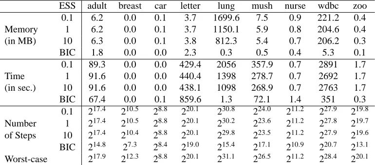
Table 1: Memory, time and number of steps (local score evaluations) used to build the cache. Re-sults for BIC and BDeu with ESS varying from 0.1 to 10 are presented.

6. Experiments

We perform experiments to show the benefits of the reduced cache and search space. Later we show some examples of the use of constraints.7 First, we use data sets available at the UCI repository (Asuncion and Newman, 2007). Lines with missing data are removed and continuous variables are discretized over the mean into binary variables. The data sets are: adult (15 variables and 30162 instances), breast (10 variables and 683 instances), car (7 variables and 1728 instances) letter (17 variables and 20000 instances), lung (57 variables and 27 instances), mushroom (23 variables and 1868 instances, denoted by mush), nursery (9 variables and 12960 instances, denoted by nurse), Wisconsin Diagnostic Breast Cancer (31 variables and 569 instances, denoted by wdbc), zoo (17 variables and 101 instances). The number of categories per variables varies from 2 to dozens in some cases (we refer to UCI for further details).

Table 1 presents the used memory in MB (first block), the time in seconds (second block) and number of steps in local score evaluations (third block) for the cache construction, using the prop-erties of Section 4. Each column presents the results for a distinct data set. In different lines we show results for BDeu with ESS equals to 0.1, 1, 10, and for BIC. The line worst-case presents the number of steps to build the cache without using Theorems 4 (for BIC/AIC) and 9 (for BDeu), which are the theorems that allow the algorithm to avoid computing every subset of parents. As we see through the log-scale in which they are presented, the reduction in number of steps has not been

exponential, but still saves a good amount of computations (roughly half of the work). In the case of the BIC score, the reduction is more significant. In terms of memory, the usage clearly increases with the number of variables in the network (lung has 57 and wdbc has 31 variables).

ESS adult breast car letter lung mush nurse wdbc zoo

Max. 0.1 2.1(4) 1.0(1) 0.7(1) 4.5(5) 0.1(2) 4.1(5) 1.2(3) 1.3(2) 1.4(3)

Number 1 2.4(4) 1.0(1) 1.0(2) 5.2(6) 0.4(2) 4.4(7) 1.7(3) 1.7(3) 1.9(4)

of Parents 10 3.3(5) 1.0(1) 1.9(2) 5.9(6) 3.0(4) 4.8(8) 2.1(3) 3.1(4) 3.4(4)

BIC 2.8(5) 1.0(1) 1.3(2) 6.3(7) 2.1(3) 4.1(4) 1.8(3) 2.7(3) 2.8(3)

Worst-case 14.0 9.0 6.0 16.0 6.0∗ 22.0 8.0 8.0∗ 16.0

Final Size 0.1 24.2 21.5 21.1 28.2 20.2 28.5 21.9 23.6 23.3

of the 1 24.8 21.9 21.6 29.0 20.8 28.9 22.4 24.9 24.4

Cache 10 26.3 23.3 23.0 210.5 210.7 29.8 23.5 212.1 28.9

BIC 29.3 ₂4.7 ₂4.5 ₂15.3 ₂11.5 ₂13.0 ₂5.6 ₂12.9 ₂10.9

Worst-case 217.9 212.3 28.8 220.1 231.1∗ 226.5 211.2 228.4∗ 220.1

Implied 0.1 254.1 213.3 26.3 2129.0 28.2 2175.7 211.6 290.3 239.3

Search 1 262.1 217.1 28.3 2144.8 233.1 2186.0 215.4 2132.7 260.3

Space 10 291.6 ₂33.2 ₂20.6 ₂176.1 ₂612.0 ₂221.8 ₂27.3 ₂375.1 ₂150.7

(approx.) BIC 271 223 210 2188 2330 2180 217 2216 2111

Worst-case 2210 290 242 2272 21441∗ 2506 272 2727∗ 2272

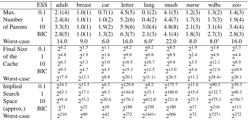
Table 2: Final cache characteristics: maximum number of parents (average by node; between parenthesis is presented the actual maximum number), actual cache size, and (approxi-mate) search space implied by the cache. Worst-cases are presented for comparison (those marked with a star are computed using the constraint on the number of parents that was applied to lung and wdbc). Results of BIC and BDeu with ESS from 0.1 to 10 are pre-sented.