Greedy Algorithms for Classiﬁcation – Consistency, Convergence Rates, and Adaptivity

(1)

Greedy Algorithms for Classification – Consistency,

Convergence Rates, and Adaptivity

Shie Mannor [email protected]

Laboratory for Information and Decision Systems Massachusetts Institute of Technology

Cambridge, MA 02139

Ron Meir [email protected]

Department of Electrical Engineering Technion, Haifa 32000, Israel

Tong Zhang [email protected]

IBM T.J. Watson Research Center Yorktown Heights, NY 10598

Editor: Yoram Singer

Abstract

Many regression and classification algorithms proposed over the years can be described as greedy procedures for the stagewise minimization of an appropriate cost function. Some examples include additive models, matching pursuit, and boosting. In this work we focus on the classification prob-lem, for which many recent algorithms have been proposed and applied successfully. For a specific regularized form of greedy stagewise optimization, we prove consistency of the approach under rather general conditions. Focusing on specific classes of problems we provide conditions under which our greedy procedure achieves the (nearly) minimax rate of convergence, implying that the procedure cannot be improved in a worst case setting. We also construct a fully adaptive procedure, which, without knowing the smoothness parameter of the decision boundary, converges at the same rate as if the smoothness parameter were known.

1. Introduction

(2)

have been addressed. For example, the notion of the margin and its impact on performance (Vapnik, 1998, Schapire et al., 1998), the derivation of sophisticated finite sample bounds (e.g., Bartlett et al., 2002, Bousquet and Chapelle, 2002, Koltchinksii and Panchenko, 2002, Zhang, 2002, Antos et al., 2002), the utilization of a range of different cost functions (Mason et al., 2000, Friedman et al., 2000, Lugosi and Vayatis, 2001, Zhang, 2002, Mannor et al., 2002a) are but a few of the recent contributions to this field.

Boosting algorithms have been demonstrated to be very effective in many applications, a success which led to some initial hopes that boosting does not overfit. However, it became clear very quickly that boosting may in fact overfit badly (e.g., Dietterich, 1999, Schapire and Singer, 1999) if applied without regularization. In order to address the issue of overfitting, several authors have recently addressed the question of statistical consistency. Roughly speaking, consistency of an algorithm with respect to a class of distributions implies that the loss incurred by the procedure ultimately converges to the lowest loss possible as the size of the sample increases without limit (a precise definition is provided in Section 2.1). Given that an algorithm is consistent, a question arises as to the rates of convergence to the minimal loss. In this context, a classic approach looks at the so-called minimax criterion, which essentially measures the performance of the best estimator for the worst possible distribution in a class. Ideally, we would like to show that an algorithm achieves the minimax (or close to minimax) rate. Finally, we address the issue of adaptivity. In computing minimax rates one usually assumes that there is a certain parameterθcharacterizing the smoothness of the target distribution. This parameter is usually assumed to be known in order to compute the minimax rates. For example, the parameterθmay correspond to the Lipschitz constant of a decision boundary. In practice, however, one usually does not know the value ofθ. In this context one would like to construct algorithms which are able to achieve the minimax rates without knowing the value ofθin advance. Such procedures have been termed adaptive in the minimax sense by Barron et al. (1999). Using a boosting model that is somewhat different from ours, it was shown by B ¨uhlmann and Yu (2003) that boosting with early stopping achieves the exact minimax rates of Sobolev classes with a linear smoothing spline weak learner, and the procedure adapts to the unknown smoothness of the Sobolev class.

The stagewise greedy minimization algorithm that is considered in this work is natural and closer to algorithms that are used in practice. This is in contrast to the standard approach of selecting a hypothesis from a particular hypothesis class. Thus, our approach provides a bridge between theory and practice since we use theoretical tools to analyze a widely used practical approach.

(3)

2. Background and Preliminary Results

We begin with the standard formal setup for supervised learning. Let(

Z,A

,P) be a probability

space and let

F

be a class of

A

measurable functions from

Z

to R. In the context of

learn-ing one takes

Z

=

X

_×

Y

where

X

is the input space and

Y

is the output space. We let S=

{(X1,Y1), . . . ,(Xm,Ym)}denote a sample generated independently at random according to the

proba-bility distribution P=PX,Y; in the sequel we drop subscripts (such as X,Y ) from P, as the argument

of P will suffice to specify the particular probability. In this paper we consider the problem of clas-sification where

Y

=_{−1,+1_}and

X

=Rd, and where the decision is made by taking the sign of a real-valued function f(x). Consider the 0₋1 loss function given by

`(y,f(x)) =I[y f(x)_≤0], (1)

where I[E]is the indicator function of the event E, and the expected loss is given by

L(f) =E`(Y,f(X)). (2) Using the notationη(x)=4P(Y =1_|X =x), it is well known that L∗, the minimum of L(f), can be achieved by setting f(x) =2η(x)₋1 (e.g., Devroye et al., 1996). Note that the decision choice at the point f(x) =0 is not essential in the analysis. In this paper we simply assume that`(y,0) =1/2, so that the decision rule 2η(x)₋1 is Bayes optimal atη(x) =1/2.

2.1 Consistency, Minimaxity and Adaptivity

Based on a sample S, we wish to construct a rule f which assigns to each new input x a (soft) la-bel f(S,x), for which the expected loss L(f,S) =E`(Y,f(S,X))is minimal. Since S is a random variable so is L(f,S), so that one can only expect to make probabilistic statements about this ran-dom variable. In this paper, we follow standard notation within the statistics literature, and denote sample-dependent quantities by a hat above the variable. Thus, we replace f(S,x)by ˆf(x). In gen-eral, one has at one’s disposal only the sample S, and perhaps some very general knowledge about the problem at hand, often in the form of some regularity assumptions about the probability distri-bution P. Within the PAC setting (e.g., Kearns and Vazirani, 1994), one makes the very stringent assumption that Yi=g(Xi)and that g belongs to some known function class. Later work considered

the so-called agnostic setting (e.g., Anthony and Bartlett, 1999), where nothing is assumed about g, and one compares the performance of ˆf to that of the best hypothesis f∗ within a given model class

F

, namely f∗=argmin_f_∈_F L(f)(in order to avoid unnecessary complications, we assume f∗ exists). However, in general one is interested in comparing the behavior of the empirical estimator

ˆ

f to that of the optimal Bayes estimator, which minimizes the probability of error. The difficulty, of course, is that the determination of the Bayes classifier gB(x) =2η(x)−1, requires knowledge

of the underlying probability distribution. In many situations, one possesses some general knowl-edge about the underlying class of distributions P, usually in the form of some kind of smoothness assumption. For example, one may assume thatη(x) =P(Y =1_|x)is a Lipschitz function, namely

|η(x)₋η(x0)_{| ≤}K_kx₋x0_kfor all x and x0. Let us denote the class of possible distributions by

P

, and an empirical estimator based on a sample of size m by ˆfm. Next, we introduce the notion of

consistency. Roughly, a classification procedure leading to a classifier ˆfnis consistent with respect

(4)

Definition 1 A classification algorithm leading to a classifier ˆfmis strongly consistent with respect

to a class of distributions

P

if for every P_∈

P

lim

m_→∞L(

ˆ

fm) =L∗, P almost surely.

If

X

_⊆Rd and

P

contains all Borel probability measures, we say that the algorithm is universally consistent.

In this work we show that algorithms based on stagewise greedy minimization of a convex upper bound on the 0₋1 loss are consistent with respect to the class of distributions

P

, where certain regularity assumptions will be made concerning the class conditional distributionη(x).

Consistency is clearly an important property for any learning algorithm, as it guarantees that the algorithm ultimately performs well, in the sense of asymptotically achieving the minimal loss pos-sible. One should keep in mind though, that consistent algorithms are not necessarily optimal when only a finite amount of data is available. A classic example of the lack of finite-sample optimality of consistent algorithms is the James-Stein effect (see, for example, Robert, 2001, Section 2.8.2).

In order to quantify the performance more precisely, we need to be able to say something about the speed at which convergence to L∗ takes place. In order to do so, we need to determine a yard-stick by which to measure distance. A classic measure which we use here is the so-called minimax rate of convergence, which essentially measures the performance of the best empirical estimator on the most difficult distribution in

P

. Let the class of possible distributions be characterized by a parameterθ, namely

P

=

P

_θ. For example, assuming thatη(x)is Lipschitz,θcould represent the Lipschitz constant. Formally, the minimax risk is given by

rm(θ) =inf

ˆ

fm

sup

P∈Pθ

E`(Y,_fˆ_m₍_X₎₎₋_L∗_,

where ˆfmis any estimator based on a sample S of size m, and the expectation is taken with respect to

X,Y and the m-sample S. The rate at which the minimax risk converges to zero has been computed in the context of binary classification for several classes of distributions by Yang (1999).

So far we have characterized the smoothness of the distribution P by a parameterθ. However, in general one does not possess any prior information aboutθ, except perhaps that it is finite. The question then arises as to whether one can design an adaptive scheme which constructs an estimator

ˆ

fm without any knowledge of θ, and for which convergence to L∗ at the minimax rates (which

assumes knowledge of θ) can be guaranteed. Following Barron et al. (1999) we refer to such a

procedure as adaptive in the minimax sense.

2.2 Some Technical Tools

We begin with a few useful results. Let{σi}mi=1be a sequence of binary random variables such that σi=±1 with probability 1/2. The Rademacher complexity of

F

(e.g., van der Vaart and Wellner,

1996) is given by

Rm(

F

)=4E sup f∈F

1 m

m

∑

i=1

σif(Xi)

,

where the expectation is over_{σi}and{Xi}. See Bartlett and Mendelson (2002) for some properties

of Rm(

F

).

(5)

Theorem 2 (Adapted from Theorem 1 in Koltchinksii and Panchenko, 2002)

Let_{X1,X2, . . . ,Xm} ∈

X

be a sequence of points generated independently at random according to a

probability distribution P, and let

F

be a class of measurable functions from

X

toR. Furthermore, letφbe a non-negative Lipschitz function with Lipschitz constantκ, such that sup_x_∈X|φ(f(x))_{| ≤}M for all f _∈

F

. Then with probability at least 1₋δ

Eφ(f(X))₋1 m

m

∑

i=1

φ(f(Xi))≤4κRm(

F

) +M r

log(1/δ) 2m

for all f _∈

F

.

For many function classes, the Rademacher complexity can be estimated directly. Results sum-marized by Bartlett and Mendelson (2002) are useful for bounding this quantity for algebraic com-position of function classes. We recall the relation between Rademacher complexity and covering numbers. For completeness we repeat the standard definition of covering numbers and entropy (e.g., van der Vaart and Wellner, 1996), which are related to the Rademacher complexity.

define the`p(Qm)distance between any two functions f and g as

`p(Qm)(f,g) = m

∑

i=1

Qm|f(xi)−g(xi)|p !1/p

.

In this case we denote the (empirical) covering number of

F

by

N

(ε,

F

, `p(Qm)). The uniform`p

X

.

In the special case p=2, we will abbreviate the notation, setting H(ε,

F

,m)_≡H2(ε,F,m). Let`m

2 denote the empirical`2norm with respect to the uniform measure on the points{X1,X2, . . . ,Xm},

namely`m

2(f,g) = m1∑ m

i=1|f(Xi)−g(Xi)|2 1/2

. If

F

contains 0, then there exists a constant C such that (see Corollary 2.2.8 in van der Vaart and Wellner, 1996)

Rm(

F

)≤

E Z ∞

0

q

log

N

(ε,

F

, `m

2)dε

C

√

m, (3)

where the expectation is taken with respect to the choice of m points. We note that the approach of

using Rademacher complexity and the`m

2 covering number of a function class can often result in tighter bounds than some of the earlier studies that employed the`m

1 covering number (for example,

(6)

2.3 Related Results

We discuss some previous work related to the issues studied in this work. The question of the consistency of boosting algorithms has attracted some attention in recent years. Jiang, following Breiman (2000), raised the questions of whether AdaBoost is consistent and whether regularization is needed. It was shown in Jiang (2000b) that AdaBoost is consistent at some point in the process of boosting. Since no stopping conditions were provided, this result essentially does not determine whether boosting forever is consistent or not. A one dimensional example was provided by Jiang (2000a), where it was shown that AdaBoost is not consistent in general since it tends to a nearest neighbor rule. Furthermore, it was shown in the example that for noiseless situations AdaBoost is in fact consistent. The conclusion from this series of papers is that boosting forever for AdaBoost is not consistent and that sometimes along the boosting process a good classifier may be found.

In a recent paper Lugosi and Vayatis (2001) also presented an approach to establishing con-sistency based on the minimization of a convex upper bound on the 0₋1 loss. According to this approach the convex cost function, is modified depending on the sample size. By making the con-vex cost function sharper as the number of samples increases, it was shown that the solution to the convex optimization problem yields a consistent classifier. Finite sample bounds are also provided by Lugosi and Vayatis (2001, 2002). The major differences between our work and (Lugosi and Vayatis, 2001, 2002) are the following: (i) The precise nature of the algorithms used is different; in particular the approach to regularization is different. (ii) We establish convergence rates and pro-vide conditions for establishing adaptive minimaxity. (iii) We consider stagewise procedures based on greedily adding on a single base hypothesis at a time. The work of Lugosi and Vayatis (2002) focused on the effect of using a convex upper bound on the 0₋1 loss.

A different kind of consistency result was established by Mannor and Meir (2001, 2002). In this work geometric conditions needed to establish the consistency of boosting with linear weak learners were established. It was shown that if the Bayes error is zero (and the oppositely labelled points are well separated) then AdaBoost is consistent.

Zhang (2002) studied an approximation-estimation decomposition of binary classification meth-ods based on minimizing some convex cost functions. The focus there was on approximation error analysis as well as behaviors of different convex cost functions. The author also studied estimation errors for kernel methods including support vector machines, and established universal consistency results. However, the paper does not contain any specific result for boosting algorithms.

All of the work discussed above deals with the issue of consistency. This paper extends our earlier results (Mannor et al., 2002a) where we proved consistency for certain regularized greedy boosting algorithms. Here we go beyond consistency and consider rates of convergence and inves-tigate the adaptivity of the approach.

3. Consistency of Methods Based on Greedy Minimization of a Convex Upper Bound

Consider a class of so-called base hypotheses

H

, and assume that it is closed under negation. We define the order t convex hull of

H

as

COt(

H

) = (

f : f(x) =

t

∑

i=1

αihi(x),αi≥0, t

∑

i=1

αi≤1,hi∈

H

)

(7)

. Moreover, since minimizing the 0₋1 loss is often intractable, we consider approaches which are based on minimizing a convex upper bound on the 0₋1 loss. The main contribution of this section is the demonstration of the consistency of such a procedure.

To describe the algorithm, let φ(x) be a convex function, which upper bounds the 0₋1 loss, namely

φ(y f(x))_≥I[y f(x)_≤0], φ(u)convex.

Specific examples forφare given in Section 3.3. Consider the empirical and true losses incurred by a function f based on the lossφ,

ˆ

A(f)=4 1 m

m

∑

i=1

φ(yif(xi)),

A(f)=4EX,Yφ(Y f(X)),

=EX{η(X)φ(f(X)) + (1−η(X))φ(−f(X))} .

Here EX,Y is the expectation operator with respect to the measure P and EX is the expectation with

respect to the marginal on X .

3.1 Approximation by Convex Hulls of Small Classes

In order to achieve consistency with respect to a large class of distributions, one must demand that the classβCO(

H

)is ‘large’ in some well-defined sense. For example, if the class

H

consists only of polynomials of a fixed order, then we cannot hope to approximate arbitrary continuous functions, since CO(

H

) also consists solely of polynomials of a fixed order. However, there are classes of non-polynomial functions for whichβCO(

H

)is large.

As an example, consider a univariate (i.e., one-dimensional) functionσ:R→[0,1]. The class of symmetric ridge functions overRd is defined as:

H

σ=4_{±σ(a>x+b),a_∈Rd,b_∈R}.

∑

i

cisgn(w>i x+bi),ci,bi∈R,wi∈Rd,

∑

i

|ci| ≤C )

(8)

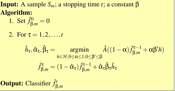
Input: A sample Sm; a stopping time t; a constantβ

Algorithm: 1. Set ˆf_β0_,_m=0 2. Forτ=1,2, . . . ,t

ˆhτ,αˆ_τ,βˆ_τ= argmin

h_∈H,0_≤α_≤1,0_≤β0_≤_β ˆ

A((1−α)_fˆτ−1

β,m +αβ0h)

ˆ

f_βτ_,_m= (1−αˆ_τ)_fˆτ−1

β,m +αˆτβˆτˆhτ

Output: Classifier ˆf_βt_,_m

Figure 1: A sequential greedy algorithm based on the convex empirical loss function ˆA.

and refers to it as the class of functions with bounded variation with respect to half-spaces. In one dimension, this is simply the class of functions with bounded variation. Note that there are several extensions to the notion of bounded variation to multiple dimensions. We return to this class of functions in Section 4.2. Other classes of base functions which generate rich nonparametric sets of functions are free-knot splines (see Agarwal and Studden, 1980, for asymototic properties) and radial basis functions (e.g., Schaback, 2000).

3.2 A Greedy Stagewise Algorithm and Finite Sample Bounds

Based on a finite sample Sm, we cannot hope to minimize A(f), but rather minimize its empirical

counterpart ˆA(f). Instead of minimizing ˆA(f)directly, we consider a stagewise greedy algorithm, which is described in Figure 1. The algorithm proposed is related to the AdaBoost algorithm in incrementally minimizing a given convex loss function. In opposition to AdaBoost, we restrict the size of the weights α andβ, which serves to regularize the algorithm, a procedure that will play an important role in the sequel. We also observe that many of the additive models introduced in the statistical literature (e.g., Hastie et al., 2001), operate very similarly to Figure 1. It is clear from the description of the algorithm that ˆf_βt_,_m, the hypothesis generated by the procedure, belongs to βCOt(

H

) for every t. Note also that, by the definition of φ, for fixed α and β the function

ˆ

A((1₋α)fˆ_βτ_,−_m1+αβh)is convex in h.

We observe that many recent approaches to boosting-type algorithms (e.g., Breiman, 1998, Hastie et al., 2001, Mason et al., 2000, Schapire and Singer, 1999) are based on algorithms sim-ilar to the one presented in Figure 1. Two points are worth noting. First, at each stepτ, the value of the previous composite hypothesis ˆf_βτ−_,_m1is multiplied by(1−α), a procedure which is usually not followed in other boosting-type algorithms; this ensures that the composite function at every step remains inβCO(

H

). Second, the parametersαandβare constrained at every stage; this serves as a regularization measure and prevents overfitting.

In order to analyze the behavior of the algorithm, we need several definitions. Forη_∈[0,1]and f _∈Rlet

(9)

Let R∗ denote the extended real line (R∗ =_R_{∪ {−}∞,+∞_}). We extend a convex function g :R→Rto a function g :R∗→R∗by defining g(∞) =limx_→∞g(x)and g(−∞) =limx_→−∞g(x).

Note that this extension is merely for notational convenience. It ensures that, fG(η), the minimizer

of G(η,f), is well-defined atη=0 or 1 for appropriate loss functions. For every value ofη∈[0,1] let

fG(η)=4argmin

f∈R∗ G(η,f) ; G

∗₍_η₎₌4_G₍_η_,_f

G(η)) = inf

f∈R∗G(η,f).

It can be shown (Zhang, 2002) that for many choices ofφ, including the examples given in Section 3.3, fG(η)>0 whenη>1/2. We begin with a result from Zhang (2002). Let f_β∗minimize A(f)

overβCO(

H

), and denote by foptthe minimizer of A(f)over all Borel measurable functions f . For simplicity we assume that foptexists. In other words

A(fopt)≤A(f) (for all measurable f ).

Our definition implies that fopt(x) = fG(η(x)).

Theorem 4 (Zhang, 2002, Theorem 2.1) Assume that fG(η)>0 whenη>1/2, and that there exist

c>0 and s_≥1 such that for allη_∈[0,1],

|η−1/2_|s_≤cs(G(η,0)₋G∗(η)).

Then for all Borel measurable functions f(x)

L(f)₋L∗_≤2c A(f)₋A(fopt)1/s, (4) where the Bayes error is given by L∗=L(2η(_·)₋1).

The condition that fG(η)>0 whenη>1/2 in Theorem 4 ensures that the optimal minimizer

fopt achieves the Bayes error. This condition can be satisfied by assuming thatφ(f)<φ(−f)for all f >0. The parameters c and s in Theorem 4 depend only on the lossφ. In general, if φis second order differentiable, then one can take s=2. Examples of the values of c and s are given in Section 3.3. The bound (4) allows one to work directly with the function A(_·)rather than with the less wieldy 0₋1 loss L(_·).

We are interested in bounding the loss L(f) of the empirical estimator ˆf_βt_,_m obtained after t

steps of the stagewise greedy algorithm described in Figure 1. Substitute ˆf_βt_,_min (4), and consider bounding the r.h.s. as follows (ignoring the 1/s exponent for the moment):

A(_fˆt

β,m)−A(fopt) = h

A(_fˆt

β,m)−Aˆ(fˆβt,m) i

+h_Aˆ₍_fˆt

β,m)−Aˆ(fβ∗) i

+hAˆ(f_β∗)₋A(f_β∗)i+hA(f_β∗)₋A(fopt)

i

. (5)

Next, we bound each of the terms separately.

The first term can be bounded using Theorem 2. In particular, since A(f) =Eφ(Y f(X)), where φis assumed to be convex, and since ˆf_βt_,_m_∈βCO(H)then f(x)∈[−β,β]for every x. It follows that

on its (bounded) domain the Lipschitz constant ofφis finite and can be written asκ_β(see explicit examples in Section 3.3). From Theorem 2 we have that with probability at least 1₋δ,

A(_fˆt

β,m)−Aˆ(fˆ t

β,m)≤4βκβRm(

H

) +φβ r

log(1/δ)

(10)

whereφ_β=4sup_f_∈_[₋_β_,_β_]φ(f). Recall that ˆf_βt_,_m_∈βCO(

H

), and note that we have used the fact that Rm(βCO(

H

)) =βRm(

H

) (e.g., Bartlett and Mendelson, 2002). The third term on the r.h.s. of (5)

can be estimated directly from the Chernoff bound. We have with probability at least 1₋δ:

ˆ

A(f_β∗)₋A(f_β∗)_≤φ_β

r

log(1/δ)

2m .

Note that f∗is fixed (independent of the sample), and therefore a simple Chernoff bound suffices here. In order to bound the second term in (5) we assume that

sup

v∈[−β,β]

φ00₍_v₎_≤_M

β<∞, (6)

whereφ00(u)is the second derivative ofφ(u).

From Theorem 4.2 by Zhang (2003) we know that for a fixed sample

ˆ

A(fˆ_βt_,_m)₋Aˆ(f_β∗)_≤8β 2_M

β

t . (7)

This result holds for every convexφand fixedβ.

The fourth term in (5) is a purely approximation theoretic term. An appropriate assumption will need to be made concerning the Bayes boundary for this term to vanish.

In summary, for every t, with probability at least 1₋2δ,

A(_fˆt

β,m)−A(fopt)≤4βκβRm(

H

) +

8β2M_β t +φβ

r

2 log(1/δ) m + (A(f

∗

β)−A(fopt)). (8)

The final term in (8) can be bounded using the Lipschitz property ofφ. In particular,

A(f_β∗)₋A(fopt) =EX n

η(X)φ(f_β∗(X)) + (1₋η(X))φ(₋f_β∗(X))o

−EX

η(X)φ(fopt(X)) + (1−η(X))φ(−fopt(X))

=EX n

η(X)[φ(f_β∗(X))₋φ(fopt(X))]

o

+EX n

(1₋η(X))[φ(₋f_β∗(X))₋φ(₋fopt(X))]

o

≤κβEX n

η(X)_|f_β∗(X)₋fopt(X)|+ (1−η(X))|f_β∗(X)−fopt(X)|

o

≤κβEX|f_β∗(X)−fβ,opt(X)|+∆β, (9)

where the Lipschitz property and the triangle inequality were used in the final two steps. Here f_β_,opt(X) =max(−β,min(β,fopt(X)))is the projection of foptonto[−β,β], and

∆β=4 sup

η∈[1/2,1]{

I(fG(η)>β)[G(η,β)−G(η,fG(η))]}.

(11)

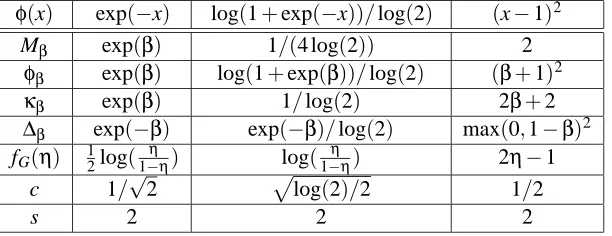
3.3 Examples forφ

We consider three commonly used choices for the convex functionφ. Other examples are presented by Zhang (2002).

exp(₋x) Exponential

log(1+exp(₋x))/log(2) Logistic loss

(x−1)2 _{Squared loss}

It is easy to see that all losses are non-negative and upper bound the 0₋1 loss I(x_≤0), where I(_·) is the indicator function. The exponential loss function was previously shown to lead to the AdaBoost algorithm (Schapire and Singer, 1999), while the other losses were proposed by Friedman et al. (2000), and shown to lead to other interesting stagewise algorithms. The essential differences between the loss functions relate to their behavior for x_{→ ±}∞.

In this paper, the natural logarithm is used in the definition of logistic loss. The division by log(2) sets the scale so that the loss function equals 1 at x=0. For each one of these cases we provide in Table 1 the values of the constants M_β,φ_β,κ_β, and∆_β defined above. We also include the values of c and s from Theorem 4, as well as the optimal minimizer fG(η). Note that the values

of∆_βandκ_βlisted in Table 1 are upper bounds (see Zhang, 2002).

φ(x) exp(₋x) log(1+exp(₋x))/log(2) (x₋1)2

M_β exp(β) 1/(4 log(2)) 2

φβ exp(β) log(1+exp(β))/log(2) (β+1)2 κβ exp(β) 1/log(2) 2β+2 ∆β exp(₋β) exp(₋β)/log(2) max(0,1₋β)2 fG(η) 1₂log(₁₋η_η) log(₁₋η_η) 2η−1

c 1/√2 plog(2)/2 1/2

s 2 2 2

Table 1: Parameter values for several popular choices ofφ.

3.4 Universal Consistency

)→0. Then the greedy algorithm of Figure

1, applied for t steps where(β2_M

β)/t→0 as m→∞, is strongly universally consistent.

Proof The basic idea of the proof is the selection ofβ=β(m)in such a way that it balances the estimation and approximation error terms. In particular, βshould increase to infinity so that the approximation error vanishes. However, the rate at whichβincreases should be sufficiently slow to guarantee convergence of the estimation error to zero as m_→∞. Letδm= _m12. It follows from (8)

that with probability smaller than 2δm

A(fˆtm

β,m)−A(fopt)>4βmκβmRm(

H

) +

8β2_mM_β_m tm

+2φ_β

r

log m

m +∆Aβ,

where∆A_β=A(f_β∗)₋A(fopt)_→0 asβ_→∞. Using the Borel Cantelli Lemma this happens finitely many times, so there is a (random) number of samples m1after which the above inequality is always reversed. Since all terms in (8) converge to 0, it follows that for every ε>0 from some time on A(_fˆt

β,m)−A(fopt)<εwith probability 1. Using (4) concludes the proof.

As a simple example for the choice ofβ=β(m), consider the logistic loss. From Table 1 we conclude that selectingβ=opm/log msuffices to guarantee consistency.

Unfortunately, no convergence rate can be established in the general setting of universal consis-tency. Convergence rates for particular functional classes can be derived by applying appropriate assumptions on the class

H

and the posterior probabilityη(x). We noted elsewhere (Mannor et al., 2002a) we used (8) in order to establish convergence rates for the three loss functions described above, when certain smoothness conditions were assumed concerning the class conditional distri-butionη(x). The procedure described in Mannor et al. (2002a) also established appropriate (non-adaptive) choices forβas a function of the sample size m. In the next section we use a different approach for the squared loss in order to derive faster, nearly optimal, convergence rates.

4. Rates of Convergence and Adaptivity – the Case of Squared Loss

We have shown that under reasonable conditions on the functionφ, universal consistency can be established as long as the base class

H

is sufficiently rich. We now move on to discuss rates of convergence and the issue of adaptivity, as described in Section 2. In this section we focus on the squared loss, as particularly tight bounds are available for this case, using techniques from the em-pirical process literature (e.g., van de Geer, 2000). This allows us to demonstrate nearly minimax rates of convergence. Since we are concerned with establishing convergence rates in a nonparamet-ric setting, we will not be concerned with constants which do not affect rates of convergence. We will denote generic constants by c,c0,c1,c0₁, etc.

We begin by bounding the difference between A(f) and A(fopt) in the non adaptive setting, where we consider the case of a fixed value ofβwhich defines the classβCO(

H

). In Section 4.2 we

use the multiple testing Lemma to derive an adaptive procedure that leads to a uniform bound over

(13)

4.1 Empirical Ratio Bounds for the Squared Loss

In this section we restrict attention to the squared loss function,

A(f) =E(f(X)₋Y)2_. Since in this case

fopt(x) =E(Y|x), we have the following identity for any function f :

i=1

(f(xi)−fopt(xi))2. (11)

Our goal at this point is to assess the expected deviation of[A(f)₋A(fopt)]from its empirical counterpart, [Aˆ(f)₋Aˆ(fopt)]. In particular, we want to show that with probability at least 1−δ, δ∈(0,1), for all f_∈

F

we have

A(f)₋A(fopt)≤c(Aˆ(f)−Aˆ(fopt)) +ρm(δ),

for appropriately chosen c andρm(δ).

For any f it will be convenient to use the notation ˆE f =4 _m1∑_im₌₁f(xi).

We now relate the expected and empirical values of the deviation terms A(f)₋A(fopt). The following result is based on the symmetrization technique and the so-called peeling method in statis-tics (e.g., Section 5.3 in van de Geer, 2000). The peeling method is a general method for bounding suprema of stochastic processes over some class of functions. The basic idea is to transform the task into a sequence of simpler bounds, each defined over an element in a nested sequence of subsets of the class (see (5.17) in van de Geer, 2000). Since the proof is rather technical, it is presented in the appendix.

Lemma 6 Let

F

be a class of uniformly bounded functions, and let X =_{X1, . . . ,Xm} be a set

of points drawn independently at random according to some law P. Assume that for all f _∈

F

, sup_x_|f(x)₋fopt(x)| ≤M. Then there exists a positive constant c such that for all q≥c, with probability at least 1₋exp(₋q), for all f _∈

F

E f(X)₋fopt(X)2≤4 ˆE f(X)−fopt(X)2+

100qM2

m +

∆2

m

6

(14)

where∆mis any number such that

m∆2_m_≥32M2max(H(∆m,

F

,m),1). (12)

Observe that∆mis well-defined since the l.h.s. is monotonically increasing and unbounded, while

the r.h.s. is monotonically decreasing.

We use the following bound from van de Geer (2000):

Lemma 7 (van de Geer, 2000, Lemma 8.4) Let

F

be a class of functions such that for all positive δ, H(δ,

F

,m)_≤Kδ−2ξ, for some constants 0<ξ<1 and K. Let X,Y be random variables defined over some domain. Let W(x,y)be a real-valued function such that_|W(x,y)_{| ≤}M for all x,y, and EY|xW(x,Y) =0 for all x. Then there exists a constant c, depending onξ,K and M only, such that

for allε_≥c/√m:

P

(

sup

g_∈F

|Eˆ_{W(X,Y)g(X)_}| (_Egˆ ₍_X₎2₎(1−ξ)/2 ≥ε

)

≤c exp(₋mε2/c2).

In order to apply this bound, it is useful to introduce the following assumption.

Assumption 1 Assume that_∃M_≥1 such that sup_x_|f(x)₋fopt(x)| ≤M for all f ∈

F

. Moreover, for all positiveε, H(ε,

F

,m)_≤K(ε/M)−2ξ_{where 0}_<_ξ_<_1.

We will now rewrite Lemma 7 in a somewhat different form using the notation of this section.

Lemma 8 Let Assumption 1 hold. Then there exist positive constants c0and c1 that depend onξ and K only, such that_∀q_≥c0, with probability at least 1₋exp(₋q), for all f _∈

F

Eˆ

(fopt(X)−Y)(f(X)−fopt(X)) ≤

1₋ξ

2 Eˆ(f−fopt)

2₊_c1M2q m

1/(1+ξ)

.

Proof Let

W(X,Y) = (fopt(X)−Y)/M ; g(X) = (f(X)−fopt(X))/M.

Using Lemma 7 we find that there exist constants c and c0 that depend onξand K only, such that

∀ε≥c/√m

P

∃g_∈

G

:_|Eˆ_{W(X,Y)g(X)_}|> 1−ξ

2 Egˆ (X)

2₊1+ξ

2 ε

2/(1+ξ)

(a)

≤ Pn_∃g_∈

G

:_|Eˆ_{W(X,Y)g(X)_}|>(_Egˆ ₍_X₎2₎(1−ξ)/2_εo

= P

(

sup

g∈G

|_Eˆ_{_W₍_X_,_Y₎_g₍_X₎_}| (_Egˆ ₍_X₎2₎(1−ξ)/2 >ε

)

(b)

≤ c exp(₋mε2/c2).

where(a)used the inequality_|ab_{| ≤}1−₂ξ_|a_|2/(1−ξ)₊1+ξ

2 |b|2/(1+ξ), and(b)follows using Lemma 7.

The claim follows by settingε=pq/m and choosing c0and c1appropriately.

(15)

Theorem 9 Suppose Assumption 1 holds. Then there exist constants c0,c1>0 that depend on ξ and K only, such that_∀q_≥c0, with probability at least 1₋exp(₋q), for all f _∈

F

A(f)₋A(fopt)≤4_ξAˆ(f)−Aˆ(fopt)+c1M 2 ξ

q

m

1/(1+ξ)

.

Proof By (10) it follows that A(f)₋A(fopt) =E(f−fopt)2. There exists a constant c00depending on K only such that in Lemma 6, we can let∆2_m=c0₀M2m−1/(1+ξ)to obtain

A(f)₋A(fopt) =E(f−fopt)2≤4 ˆE(f−fopt)2+M2(100q/m+c00m−1/(1+ξ)) (13) with probability at least 1₋exp(₋q)where q_≥1. By (11) we have that

[Aˆ(f)₋Aˆ(fopt)] =2 ˆE(fopt(X)−Y)(f(X)−fopt(X)) +Eˆ(f(X)−fopt(X))2.

Using Lemma 8 we have that there exist constants c0₁_≥1 and c0₂that depend on K andξonly, such that for all q_≥c0₁, with probability at least 1₋exp(₋q):

Eˆ

(fopt(X)−Y)(f(X)−fopt(X)) ≤

1₋ξ

2 Eˆ(f−fopt) 2₊_c0

2M2

q

m

1/(1+ξ)

.

Combining these results we have that with probability at least 1₋e−q:

[_Aˆ₍_f₎₋_Aˆ₍_f_opt_{)] =} _{2 ˆ}_E

(fopt(X)−Y)(f(X)−fopt(X)) +Eˆ(f(X)−fopt(X))2

≥ ξEˆ(f₋fopt)2−2c02M2

q

m

1/(1+ξ)

. (14)

From (13) and (14) we obtain with probability at least 1₋2 exp(₋q):

A(f)₋A(fopt)≤ 4_ξ[Aˆ(f)−Aˆ(fopt)] +8_ξc02M2

q

m

1/(1+ξ)

+M2(100q/m+c0₀m−1/(1+ξ)).

Note that Assumption 1 was used when invoking Lemma 6. The theorem follows from this

inequal-ity with appropriately chosen c0and c1.

4.2 Adaptivity

In this section we let f be chosen from βCO(

H

)≡β

F

, where β will be determined adaptively based on the data in order to achieve an optimal balance between approximation and estimation errors. In this case, sup_x_|f(x)_{| ≤}βM where h_∈

H

are assumed to obey sup_x_|h(x)_{| ≤}M. We first need to determine the preciseβ-dependence of the bound of Theorem 9. We begin with a definition followed by a simple Lemma, the so-called multiple testing Lemma (e.g., Lemma 4.14 in Herbrich, 2002).

Definition 10 A testΓis a mapping from the sample S and a confidence levelδto the logical values

(16)

Lemma 11 Suppose we are given a set of testsΓ=_{Γ1, . . . ,Γr}. Assume further that a discrete

probability measure P =_{pi}r_i₌₁ over Γ is given. If for every i∈ {1,2, . . . ,r} and δ∈(0,1),

P_{Γi(S,δ)} ≥1−δ, then

P_{Γ1(S,δp1)∧ ··· ∧Γr(S,δpr)} ≥1−δ.

We use Lemma 11 in order to extend Theorem 9 so that it holds for allβ. The proof again relies on the peeling technique.

Theorem 12 Let Assumption 1 hold. Then there exist constants c0,c1>0 that depend onξand K only, such that_∀q_≥c0, with probability at least 1₋exp(₋q), for allβ_≥1 and for all f _∈β

F

we have

A(f)₋A(fopt)≤4_ξAˆ(f)−Aˆ(fopt)+c1β2M2

q+log log(3β) m

1/(1+ξ)

.

Proof For all s=1,2,3, . . ., let

F

s=2s

F

. Let us define the testΓs(S,δ)to be TRUE if

A(f)₋A(fopt)≤ 4_ξAˆ(f)−Aˆ(fopt)+_ξc22sM2

log(1/δ) m

₁₊1_ξ

for all f _∈

F

s and FALSE otherwise. Using Theorem 9 we have that P(Γs(S,δ))≥1−δ. Let

ps= _s₍_s1₊₁₎, noting that∑∞s=1ps=1 and by Lemma 11 we have that

P{Γs(S,δps)for all s} ≥1−δ.

Consider f ∈β

F

for someβ≥1. Let s=_blog₂βc+1, we have that P

n

∀s : Γs(S,_s₍_sδ₊₁₎) o

≥1−δ

so that with probability at least 1₋δwe have that:

A(f)₋A(fopt)≤4_ξAˆ(f)−Aˆ(fopt)+c

0

ξ22sM2

log(s2_δ+s) m

!1/(1+ξ)

≤4_ξ_ˆ

A(f)₋Aˆ(fopt)+c1_ξβ2M2

log log(3β) +q m

1/(1+ξ)

,

where we set q=log(1/δ)and used the fact that 2s−1_≤β_≤2s.

Theorem 12 bounds A(f)₋A(fopt)in terms of ˆA(f)−Aˆ(fopt). However, in order to determine overall convergence rates of A(f)to A(fopt)we need to eliminate the empirical term ˆA(f)₋_Aˆ₍_fopt₎_. To do so, we first recall a simple version of the Bernstein inequality (e.g., Devroye et al., 1996) together with a straightforward consequence.

Lemma 13 Let_{X1,X2, . . . ,Xm}be real-valued i.i.d. random variables such that|Xi| ≤b with

prob-ability one. Letσ2=Var[X1]. Then, for anyε>0

P

(

1 m

m

∑

i=1

Xi−E[X1]>ε )

≤exp

− mε

2 2σ2₊_2bε_/₃

(17)

Moreover, ifσ2≤c0bE[X1], then for all positive q, there exists a constant c that depends only on c0 such that with probability at least 1₋exp(₋q)

1 m

m

∑

i=1

Xi≤cE[X1] +

bq m ,

where c is independent of b.

Proof The first part of the Lemma is just the Bernstein inequality (e.g., Devroye et al., 1996). To show the second part we need to bound from above the probability that(1/m)∑m

i=1Xi>cE[X1] + bq/m. Setε= (c₋1)E[X1] +bq/m. Using Bernstein’s inequality we have that

P

(

1 m

m

∑

i=1

Xi−E[X1]>(c−1)E[X1] +

bq m

)

≤exp

− mε

2 2σ2₊_2bε_/₃

≤exp

− mε

2 2c0bE[X1] +2bε/3

(a)

≤exp

−m_bε ≤exp(₋q),

where(a) follows by choosing c large enough so that 2c0 < 1

3(c−1), implying that 2c0bE[X1]<

bε/3.

Next, we use Bernstein’s inequality in order to bound ˆA(f)₋Aˆ(fopt).

such that

ˆ

A(_fˆ_q_{) +}_γ_q₍_βˆ

q)≤inf

β≥1

inf

f∈βF

ˆ

A(f) +2γq(β)

. (16)

This procedure is similar to the so-called structural risk minimization method (Vapnik, 1982), except that the minimization is performed over the continuous parameterβrather than a discrete hypothesis class counter. Observe that ˆβqand ˆfqare non unique, but this poses no problem.

We can now establish a bound on the loss incurred by this procedure.

Theorem 15 Let Assumption 1 hold. Choose q0>0 and assume we compute ˆfq0 using (16). Then

there exist constants c0,q0>0 that depend onξand K only, such that∀m≥q≥max(q0,c0), with probability at least 1₋exp(₋q),

A(_fˆ_q

0)≤A(fopt) +c1

q q0

1/(1+ξ)

inf

β≥1

inf

f∈βFA(f)−A(fopt) +γq(β)

.

Note that since for any q, γq(β) =O((1/m)1/(1+ξ)), Theorem 15 provides rates of convergence

in terms of the sample size m. Observe also that the main distinction between Theorem 15 and Theorem 12 is that the latter provides a data-dependent bound, while the former establishes a so-called oracle inequality, which compares the performance of the empirical estimator ˆfq0 to that

of the optimal estimator within a (continuously parameterized) hierarchy of classes. This optimal estimator cannot be computed since the underlying probability distribution is unknown, but serves as a performance yard-stick.

Proof (of Theorem 15) Considerβq≥1 and fq∈βq

F

such that

A(fq)−A(fopt) +2γq(βq)≤inf

β≥1

inf

f∈βFA(f)−A(fopt) +4γq(β)

. (17)

Note thatβq and fq determined by (17), as opposed to ˆβq and ˆfq in (16), are independent of the

data. Using Lemma 14, we know that there exists a constant c0₂ such that with probability at least 1₋exp(₋q):

ˆ

A(fq)−Aˆ(fopt) +2γq(βq)≤c02inf

β≥1

inf

f∈βFA(f)−A(fopt) +γq(β)

(19)

From (16) we have

ˆ

A(fˆq0)−Aˆ(fopt) +γq0(βˆq0)

(a)

≤ Aˆ(fq)−Aˆ(fopt) +2γq0(βq)

(b)

≤ Aˆ(fq)−Aˆ(fopt) +2γq(βq)

(c)

≤ c0₂inf

β≥1

inf

f_∈βFA(f)−A(fopt) +γq(β)

. (19)

Here (a) results from the definition of ˆfq0, (b) uses q≥q0, and (c) is based on (18). We then

conclude that there exist constants c0₀,c0₁>0 that depend onξand K only, such that_∀q_≥c0₀, with probability at least 1₋exp(₋q):

A(fˆq0)−A(fopt)

(a)

≤ c0₁[Aˆ(fˆq0)−Aˆ(fopt) +γq(βˆq0)]

(b)

≤ c0₁

q q0

1/(1+ξ)

[_Aˆ₍_fˆ_q

0)−Aˆ(fopt) +γq0(βˆq0)]

(c)

≤ c0₁c0₂

q q0

1/(1+ξ)

inf

β≥1[finf∈βFA(f)−A(fopt) +γq(β)].

Here(a) is based on Theorem 12,(b) follows from the definition ofγq(β) and(c) follows from

(19).

4.3 Classification Error Bounds

Theorem 15 established rates of convergence of A(fˆ)to A(fopt). However, for binary classification problems, the main focus of this work, we wish to determine the rate at which L(_fˆ₎_{converges to} the Bayes error L∗. However, from the work of Zhang (2002), reproduced as Theorem 4 above, we immediately obtain a bound on the classification error.

Corollary 16 Let Assumption 1 holds. Then there exist constants c0,c1>0 that depend onξand K only, such that_∀m_≥q_≥max(q0,c0), with probability at least 1−exp(−q),

L(fˆq0)≤L∗+c0

q q0

1/2(1+ξ)

inf

β≥1

inf

f∈βF A(f)−A(fopt)

+γq(β) 1/2

. (20)

Moreover, if the conditional probabilityη(x)is uniformly bounded away from 0.5, namely_|η(x)₋ 1/2_{| ≥}δ>0 for all x, then with probability at least 1₋exp(₋q),

L(fˆq0)≤L∗+c1

q q0

1/(1+ξ)

inf

β≥1

inf

f∈βF(A(f)−A(fopt)) +γq(β)

.

Proof The first inequality follows directly from Theorems 4 and 15, noticing the s=2 for the least squares loss. The second inequality follows from Corollary 2.1 of Zhang (2002). According to this corollary

L(fˆq0)≤L∗+2c inf

δ>0

E_|_η₍_x₎₋1

2|<δ(

ˆ

fq0−fopt)

21/2₊_c01

δ(A(fˆq0)−A(fopt))

(20)

H

. Then there exists a constant K that depends on C and V only such that

log

N

2(ε,βCO(

H

N(B) =

f : Z

Rdkωk1|

˜

f(ω)_|dω_≤B

,

consisting of all functions with a Fourier transform which decays sufficiently rapidly. Define the approximating class composed of neural networks with a single hidden layer,

H

n= (

f : f(x) =c0+

n

∑

i=1

ciφ(v>i x+bi), |c0|+ n

∑

i=1

|ci| ≤B )