Multiscale Adaptive Representation of Signals: I. The Basic Framework

Multiscale Adaptive Representation of Signals: I.

The Basic Framework

Cheng Tai [email protected]

PACM, Princeton University Princeton, NJ 08544, USA

Weinan E [email protected]

School of Mathematical Sciences and BICMR Peking University and

Department of Mathematics and PACM Princeton University

Princeton, NJ 08544, USA

Editor: Tong Zhang

Abstract

We introduce a framework for designing multi-scale, adaptive, shift-invariant frames and bi-frames for representing signals. The new framework, called AdaFrame, im-proves over dictionary learning-based techniques in terms of computational effi-ciency at inference time. It improves classical multi-scale basis such as wavelet frames in terms of coding efficiency. It provides an attractive alternative to dictio-nary learning-based techniques for low level signal processing tasks, such as com-pression and denoising, as well as high level tasks, such as feature extraction for ob-ject recognition. Connections with deep convolutional networks are also discussed. In particular, the proposed framework reveals a drawback in the commonly used approach for visualizing the activations of the intermediate layers in convolutional networks, and suggests a natural alternative.

Keywords: AdaFrame, Dictionary Learning, Wavelet Frames/Bi-frames

1. Introduction

It is now well acknowledged that sparse and overcomplete representations of data play a key role in many signal processing applications. The ability to represent a signal as a sparse linear combination of a few atoms from a possibly overcomplete dictionary lies at the heart of many applications including image/audio compression, denoising, as well as higher level tasks such as object recognition.

data can be written as a sparse linear combination of the dictionary atoms. More specifically, given the data represented as a matrixX, one finds the dictionary matrix

D and coefficient matrix C simultaneously by solving:

min

D,C kX−DCk

2

2+λkCk1. (1)

The solution is usually obtained by solving alternatively the minimization problem for

Dand the sparse coding problem forC with the other variable being kept fixed. After obtaining D, inference can be made by solving a sparse coding problem. Different dictionary learning models differ in the way the dictionary D is updated. Examples include: MOD (Engan et al., 1999a), K-SVD (Aharon et al., 2006) and their variants. Dictionary learning techniques have been successfully applied to some low level image and video processing tasks, such as image/video denoising (Elad and Aharon, 2006), compression (Bryt and Elad, 2008a; Engan et al., 1999b), inpainting (Mairal et al., 2008) and other restoration tasks (Mairal et al., 2007) with state-of-the-art performances. In addition, dictionary learning and sparse coding techniques have been very popular in high level object recognition tasks where their function is to extract features from raw data. These techniques have been used successfully to extract visual features in Ranzato et al. (2007); Lee et al. (2009); Jarrett et al. (2009). At the other end are the more traditional methodologies of designing analytic tight frames, such as Fourier basis, wavelet frames and bi-frames (Daubechies et al., 2003), curvelets (Candes and Donoho, 2000), contourlets (Do and Vetterli, 2002), etc. These analytic tight frames are robust, easy to use and computationally efficient.

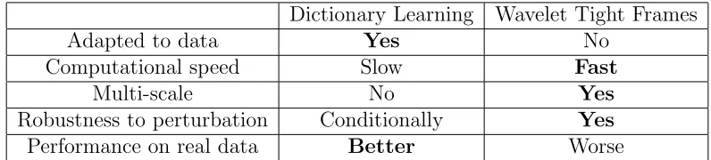
In some sense the analytic tight frames can also be viewed as a dictionary. The set of signals is a particular space of functions. A dictionary is found that gives rise to the optimal representation and approximation of the signals in that function class. The resulted dictionary is highly structured, and in particular, when used into applications, the dictionary atoms are never explicitly used. However, the two approaches do differ fundamentally in several aspects (see Table 1).

• Computational cost. For dictionary learning, the computational cost con-sists of two parts: the one time cost of learning the dictionary atoms and the repeated cost of solving the sparse coding problem for the test signal at infer-ence time. Among the two, it is the latter that prevents it from being used in real time situations. Despite the efforts devoted to seeking more efficient sparse coding algorithms (Daubechies et al., 2004; Lee et al., 2006; Beck and Teboulle, 2009), none of the available techniques is efficient enough for large scale visual feature extraction. In fact, assuming that the signal x is of length N and the trained dictionaryD∈_Rm×N _{is stored and used explicitly, then computing Dx}

learning procedure requires solving a non-convex optimization problem, limiting dictionary atoms to low dimensions. Partly because of this, in image processing applications, dictionary atoms are only obtained for small image patches.

• Multi-scale features. Dictionaries as obtained by MOD and K-SVD operate at a single small scale. Since the dictionary atoms are limited to small sizes, there is not much room for multi-scale features. Past experience with wavelets has taught us that often times it is beneficial to process signals at several scales, and operate at each scale separately.

• Artifacts. In low level tasks such as image compression, the dictionary learning approach operates in a patch by patch manner, which produces visually unpleas-ant block effects along the boarders of the patches (Bryt and Elad, 2008a). Post processing is often needed to remove these artifacts (Bryt and Elad, 2008b).

Dictionary Learning Wavelet Tight Frames

Adapted to data Yes No

Computational speed Slow Fast

Multi-scale No Yes

Robustness to perturbation Conditionally Yes

Performance on real data Better Worse

Table 1: Comparison between dictionary learning and wavelet tight frames

Given the relative features of dictionary learning and wavelet tight frames, it is natural to ask whether one can design bases that have the benefits of both and avoid the problems. In other words, can one design bases that are adapted to the data but at the same time have the multi-scale structure that is essential for the efficient algorithms for wavelet tight frames?

We propose a framework of constructing adaptive frames and bi-frames (abbrevi-ated as AdaFrame). This framework gives multi-scale, sparse representations of the signal, with an efficiency comparable to that of the wavelets at inference time.

The proposed framework is formally similar to the first few layers of a convolu-tional network. As a byproduct, we show that the proposed framework gives a better way of visualizing the activations of the intermediate layers of a neural net in terms of reconstruction error.

The framework presented here is best suited for datasets such that each data point has some structure. Obvious examples include time series, images and videos. However, as in the case of wavelets, it is also possible to extend this kind of ideas to less structured data such as graphs, etc (Coifman and Maggioni, 2006).

a similar objective and build upon similar mathematical foundations, but our work greatly extends the model proposed in Cai et al. (2014) where a sufficient condition for perfect reconstruction is replaced by a sufficient and necessary condition and the tight frame is extended to bi-frame, which is much more flexible.

Most examples discussed in this paper are still of the low level image processing type. In a subsequent paper, we will discuss more thoroughly higher level tasks such as image classification.

The organization of this paper is as follows. In section 2, we introduce shift-invariant frames and bi-frames. In section 3, we introduce the adaptive construction of invariant frames. In section 4, we introduce the adaptive construction of shift-invariant bi-frames. In section 5, we discuss multi-level constructions. In section 6, we give some simple illustrative examples of the adaptively constructed frames and bi-frames. In section 7, we discuss the connection with predefined wavelets and wavelet frames. In section 8, we discuss applications to image processing and image classifica-tion. In section 9, we discuss connection with deconvolutional nets and reconstruction of input data from features in the intermediate layers of the convolutional nets. Some conclusions are drawn in section 10.

2. Shift-invariant Frames and Bi-frames

An important starting point is the concept of multi-resolution analysis (MRA) intro-duced in Mallat (1989) and Meyer (1995), of which wavelets are particularly popular examples. One main advantage of MRA is that it comes naturally with fast decompo-sition and reconstruction algorithms, and this has been essential for making wavelets a practical tool in signal processing (Daubechies et al., 2003; Shen, 2010). Although our work builds upon the theory of wavelet frames in the continuous setting, we decide to introduce our model in a purely discrete setup. This has the advantage that it is more direct and more easily linked with existing machine learning models, including dictionary learning and convolutional networks. However, as noted in Han (2010), there is a canonical link between affine systems in the continuous setting and fast algorithms in the discrete framework.

The signals and the filters are all assumed to be discrete sequences inl2(Zd), where d is the dimension. For audio, image and video signals,d = 1,2,3 respectively. First let us define the up- and down-sampling operators. Let M be an integer. The (one dimensional) down-sampling and up-sampling operator are defined by:

[v ↓M](n) :=v(M n), n∈Z

[↑v](n) :=

v(k), n=M k, k∈_Z

0, otherwise

(2)

respectively, forv ∈l2(Z). M is the decimation factor. Similarly if d >1, denote the

decimation factor in each dimension byM1, M2,· · · , Md. For convenience we define a

is M = 2I. We call M the sampling matrix and use the same notation as in (2) where M n is understood as the matrix-vector multiplication. In general M can be an invertible matrix whose entries are positive integers or rational numbers that are greater than 1.

Key to the decomposition and reconstruction algorithms are the transition and subdivision operators. For a data sequence v ∈l2(Zd), a finitely supported filter a∈ l2(Zd) and a sampling matrix M ∈Rd×d, the transition operator Ta :l2(Zd)7→l2(Zd)

is defined by

(Ta,Mv)(n) :=↓M [v∗a](n) =

X

k∈Zd

v(k)a(k−M n), (3)

the subdivision operator Sa:l2(Zd)7→l2(Zd) is defined by

(Sa,Mv)(n) := |det(M)|[a∗(↑v)](n) =|det(M)|

X

k∈Zd

v(k)a(n−M k). (4)

To make the notations more concise, we omit M in the subscript.

Given a set of finitely supported filters A = {a1,· · · , am} and the coefficient

sequencev ∈l2(Zd), which could be the input signal itself or the coefficients computed

at some decomposition level, we compute coefficients of the next level by

vl=Talv, l = 1,· · · , m. (5)

With this notation, the one-level decomposition operatorWA:l2(Zd)7→l2(Zd)⊕ · · · ⊕l2(Zd)

| {z }

m times

is defined as:

WAv :={v1,· · · , vl}={Ta1v,Ta2v,· · · ,Tamv}. (6)

Given a set of finitely supported filtersB ={b1,· · · , bm}, the one-level reconstruction

operator Rb :l2(Zd)⊕ · · · ⊕l2(Zd)

| {z }

m times

7→l2(Zd) is defined as

RB(v1,· · · , vm) := m

X

l=1

Sblvl (7)

In wavelet frames, the filters A used for decomposition and the filters B used for reconstruction are connected by : bl(·) = al(−·), l = 1,· · ·, m, where al(−·) means

flip the entries of al along each dimension. But this does not have to be the case: A

and B can be different and together they constitute a bi-frame.

The main requirement is that of perfect reconstruction, by which we mean:

RBWAv =v ∀v ∈l2(Zd). (8)

Theorem 1 (Ron and Shen, 1997) Let M ∈ _Rd×d _{be a sampling matrix, let A =}

{a1,· · · , am} and B = {b1,· · · , bm} be two sets of finitely supported sequences in

l2(Zd). Then the perfect reconstruction property

RBWAv =v, ∀v ∈l2(Zd) (9)

holds if and only if, for all k, j∈_Zd_,

m

X

l=1

X

n∈Zd

al(M n+j)bl(k+M n+j) = |det(M)|−1δk (10)

where δk = 1 if k= 0 and δk = 0 otherwise.

In the case of wavelet tight frames, bl(·) = al(−·), l = 1,· · · , m, and we have:

Theorem 2 (Ron and Shen, 1997) Let M ∈ _Rd×d _{be a sampling matrix, let A =}

{a1,· · · , am} be a set of finitely supported sequences in l2(Zd). Then the perfect

re-construction property

RAWAv =v, ∀v ∈l2(Zd). (11)

holds if and only if, for all k, j∈_Zd_,

m

X

l=1

X

n∈_Zd

al(M n+j)al(k+M n+j) =|det(M)|−1δk (12)

In particular, if the data are real numbers and no down-sampling is performed, then the perfect reconstruction condition (12) becomes

m

X

i=1

X

n∈Zd

ai(k+n)ai(n) = δk,∀k ∈Zd. (13)

The proof of Theorem 1 and Theorem 2 can be found in Daubechies et al. (2003). For completeness, we give a direct proof for the discrete case in the appendix. These conditions are referred to as the unitary extension principle (UEP) in wavelet frame theory.

As an example, the linear B-spline wavelet tight frame used in many image restora-tion tasks is constructed via the UEP. Its associated filters are :

a1 =

1

4(1,2,1)

T

; a2 =

√

2

4 (1,0,−1)

T

; a3 =

1

4(−1,2,−1)

T

.

3. Adaptive Construction of Frames

Given a set of signalsX ={x1,· · · , xN}, the goal is to construct wavelet frames that

are adapted to this set of signals in the sense that signals in the given set have a sparse representation.

Define Qto be the set of filters that satisfy the UEP condition:

Q=n{ai}mi=1 :

m

X

l=1

X

n∈Zd

al(M n+j)al(M n+k+j) =|det(M)|−1δk, ∀k, j ∈Zd

o

.

(14) Filters in this set generate a wavelet frame that provide a faithful representation for all signals in l2(Zd). However, we are not interested in all signals in l2(Zd). We are

only interested in X. Among all filters in Q, we want to select the one that is most adapted to X.

In image restoration tasks, we are mostly interested in wavelet frames that give rise to a sparse representation of the input signal. Therefore we will use sparsity as our guiding principle for selecting the filters. Other guiding principles such as the discriminative criterion can also be used. But in this paper, we will focus on sparsity. Let Φ be a sparsity-inducing function. Examples of Φ include the l1 norm, l0

“norm”, or the Huber loss function defined (component-wise) by:

Lδ(x) =

₁

2x

2_{, |x| ≤δ} δ(|x| − 1

2δ), otherwise

. (15)

Given the dataX, the adaptive filters are chosen by solving the following optimization problem:

min

a1,···,am

N

X

j=1

m

X

i=1

Φ(vi,j)

subject to vi,j =Taixj, i= 1,· · · , m

{ai}mi=1 ∈ Q

(16)

In the following, without loss of generality, we will assume that there is only one data point in the signal set, i.e. N = 1, and we will omit the subscript j.

To be specific, we use l1 norm as the measurement of sparsity and we will note

the changes required if the l0 norm is used. The above problem then becomes

min

a1,···,am

m

X

i=1

kTaixk1

{ai}mi=1 ∈ Q

(17)

real symmetric matrixG, let us denote byT r(G, k) the sum of entries along thek-th sub-diagonal. For example, T r(G,0) is the usual trace of G. Let A:= (a1,· · · , am).

Then the constraint {ai}mi=1 ∈ Q is equivalent to

T r(AAT, k) = δk, k = 0,· · · , r−1.

To see a nontrivial example where this constraint is satisfied, take an orthorgonal matrix U ∈_Rr×r_{, and let a}

i = √1_rU·,i, i= 1,· · · , m, where U·,i means thei-th column

of U. However, in general, the algebraic constraint above is difficult to deal with. Note also that this optimization problem is not convex.

We use the split Bregman algorithm (Goldstein and Osher, 2009) to solve (17). Introduce the auxiliary variable D = (d1,· · · , dm) where di = Taix, i = 1,· · · , m.

Define the normkDk1,1 :=

Pm

i=1kdik1. Then (17) is equivalent to:

min

A,D kDk1,1

subject to D=WAx

A∈ Q

(18)

Applying the split Bregman method, we obtain the following algorithm:

Algorithm 1 Adaptive construction of frames

1: Input: x.

2: Initialize k= 0, B =0, A=A0_{, D =W}

A0x.

3: while “not converge” do

4: Dk+1 ←arg minDkDk1,1+ η₂kD−WAkx−Bkk2_F

5: Ak+1 _{←arg min}

AkWAx−Dk+1+Bkk2F s.t. A∈ Q.

6: Bk+1 _←Bk_+W

Ak+1−Dk+1.

7: k ←k+ 1

8: return Ak

To implement the algorithm, we must be able to solve each of the subproblems listed in steps 4, 5 and 6.

To solve the subproblem for D, note that the problem decouples for eachdi, i=

1,· · · , m. In fact,

dk_i+1 = arg min

d

kdk1+ η

2kTakix−d+b

k

ik

(19)

for i= 1,· · · , m. It is easy to see that (19) has a closed form solution given by

dk_i+1 = shrink(T_ak ix+b

k

i,

1

(a) (b) (c)

Figure 1: (a) The input image.(b) The filters learned using Algorithm 1, m= 20, r= 20.(c) The Fourier spectrum of the corresponding filters. Note the first filter is a low-pass filter, all other filters are high-pass filters as can be seen from the Fourier spectrum. The second and third filter look like edge detectors along the axis. Other filters detect oscillations along different directions.

where the function shrink :_R7→_R is defined as

shrink(x, a) =

(|x| −a)sign(x), if |x|> a

0, otherwise . (21)

When shrinkage-operator acts on a vector, it acts on each component of the vector according to (21).

The subproblem for updating A is most problematic due to the constraint. We use the interior-point method for this part of the algorithm. There is no guarantee of a global solution to this subproblem.

The update for B is straightforward. This is analogous to the step of “adding the noise back” in the ROF model for denoising (Osher et al., 2005).

Among the three subproblems, the update of Ais the most time consuming. But as is observed by many authors, it is not necessary to solveAto full convergence, the intuitive reason being that if the error of the solution to the subproblem is smaller than kBk _−Bk−1_{k, the extra accuracy will be wasted. In fact, for updating A, we}

only run a few steps of the interior-point iterations and we still observe numerical convergence.

If we use the l0 “norm” as the measurement of sparsity, the only change needed

in the above algorithm is in theDstep, where the soft-shrinkage operator is replaced by hard-thresholding defined as:

Hard(x, a) =

x, if |x|> a

0, otherwise . (22)

In some applications such as object recognition, perfect reconstruction is unnec-essary. Instead, writing the input signal as a sparse linear combination of a few dictionary atoms is only a means to extract features to be used by other learning algorithms. Sparse coding has been quite popular in serving this purpose for visual object recognition tasks. In this case, it is possible to relax the constraint in (17). In-stead of solving the constrained minimization problem, we can use a penalty method to solve an unconstrained problem. For example, in 1D, we can solve

min

A m

X

i=1

kWAxk1,1+η

X

k

(T r(AAT, k)−δk)2 (23)

where η is a parameter that depends on our tolerance on the reconstruction error. This unconstrained problem is relatively easy to solve using first-order optimization methods.

The optimization problem may appear similar to reconstruction ICA (RICA)proposed in Le et al. (2011), but they are fundamentally different. There proposed model guar-antees perfect reconstruction while RICA approximates the input signal. Perfect reconstruction in RICA can only be achieved in the limit where the weight of the reconstruction term goes to infinity. In addition, RICA does not have a multi-scale structure which is essential in wavelet tight frames. The goals of RICA and AdaFrame are different, in ICA, the goal is to find independent sources where as in AdaFrame, the goal is to build a wavelet tight frame that sparsely represent the signal.

4. Adaptive Construction of Bi-frames

In this section, we introduce the adaptive construction of wavelet bi-frames. Com-pared with the wavelet frames, the bi-frames offer two distinct advantages: The first is that the constraint for the filters becomes bi-linear making it easier to construct the filters. The second is that the added redundancy introduces more flexibity. These prove to be very important in practice.

Let Q denote the set of pairs A and B, A = (a1,· · · , am), B = (b1,· · · , bm), that

satisfy (10):

Q:=n(A, B) :

m

X

l=1

X

n∈Zd

al(M n+j)bl(k+M n+j) =|det(M)|−1δk, ∀k, j ∈Zd

o

(24) We want to find filter pairs (A, B) with desired properties while respect the constraint (A, B)∈ Q. As before we will only consider sparsity. Given the dataxand a sampling matrix M, we aim to solve :

min

A,B kWAxk1,1

subject to (A, B)∈ Q

The constraint (A, B)∈ Qin bi-linear inA andB. Let us first count the number of equations.

We start with the simplest case where the signals and the filters are one dimen-sional. Let A, B be defined as before and assume that each filter ai, bi, i = 1,· · · , m

has support size r. Given the decimation factor M, define

S(r) := {(k, γ) :∃n∈_Z,1≤M n+k+γ ≤r,1≤M n+γ ≤r}, (26)

then each (k, γ)∈ S(r) constitutes an equation. This gives

|S(r)|= (2r−M)M. (27)

This is the total number of equations. The total number of unknowns in A and B is 2rm. Therefore for (10) to have a solution, we expect:

2rm≥(2r−M)M. (28)

In the general case where the signals and the filters live in d dimensions, we can do a similar counting. Assume the support size of the filter ai, bi, i = 1,· · · , m is

r = (r1,· · · , rd), and assume that the sampling matrix is M = Diag(M1,· · · , Md).

Let

S(r) :={(k, γ)∈_Zd _{:∃n ∈}

Zd,1≤M n+k+γ ≤r,1≤M n+γ ≤r}, (29)

where the inequality is understood component-wise. Each (k, γ)∈ S(r) gives rise to an equation. The total number of equations is

|S(r)|=

d

Y

i=1

(2ri−Mi)Mi. (30)

The number of unknowns in a and b is 2mQd

i=1ri. Hence to have a solution to (10),

we expect:

2m

d

Y

i=1

ri ≥ d

Y

i=1

(2ri−Mi)Mi. (31)

Two cases are of special interest.

• Redundant case. In this case, the number of filters m is large. The number of decomposition coefficients is larger than the size of the input signal. Hence we call this the redundant case. For the optimization problem, we have more unknowns than equations. In particular, if m≥2M −M2_{/r in one dimension,}

andmQd

i=1ri ≥

Qd

i=1(2ri−Mi)Mi inddimensions, for mostA, we expect (10)

as a set of linear equations for B, to have a solution. Therefore, we can design

• Critically down-sampled case. In this case, the number of filtersmis small. The number of decomposition coefficients is the same as that of the input signal (depending on the boundary conditions). Hence we call this thecritically

down-sampled case. For example, in one dimension, m = M. In this down-sampled

case, for a typical A, it is likely that (10), as a linear system for B, does not have a solution. This means that we must consider A and B simultaneously.

4.1 Redundant Case

4.1.1 Design of the Decomposition Filters

As discussed above, we can design A in the first phase, and then choose B that satisfies the linear constraint (25) in the second phase.

However, the choice of A has a significant impact on the condition number of (25). Hence some constraints should be added. While there are a lot of flexibilities, we propose the following formulation:

min

A kWAxk1,1

subject to ATA=I

(32)

The additional constraint AT_{A = I is chosen based on the consideration that the}

filters are most incoherent among themselves.

To solve (32) numerically, we apply the split Bregman method. But we need to handle the extra orthogonality constraint as well. To this end, we introduce the auxiliary variable P =A as a means to split the orthogonality constraint. This trick has been used in other problems, see for example Lai and Osher (2014). The problem then becomes:

min

A,D,P kDk1,1

subject to D=WAx, P =A, PTP =I.

(33)

The algorithm is then:

Algorithm 2 Adaptive construction of bi-frames: redundant case

1: Input: x.

2: Initialize k= 0, F =0, C =0, A=A0, D =WA0x, P =A. 3: while “not converge” do

4: for n=1:N do

5: Dk+1 ←arg minD kDk1,1+η₂kD−WAkx−Fkk2_F

6: Ak+1 ←arg minA ηkWAx−Dk+1+Fkk2F +λkA−Pk+Ckk2F 7: Pk+1 ←arg minP kAk+1−P +Ckk2F s.t. PTP =I

8: Fk+1 _←Fk_+W

Ak+1x−Dk+1.

9: Ck+1 _←Ck_+Ak+1_−Pk+1

10: k ←k+ 1

To implement the algorithm, we must be able to solve each of the subproblems for D, A and P. Updating D is the same as in Algorithm 1. The subproblem for

A is a quadratic program. It can be decoupled into m smaller problems, each of which involves one column of A. Writing D = (d1,· · · , dm), P = (p1,· · · , pm),

C = (c1,· · · , cm) andF = (f1,· · · , fm), we can perform the optimization in a column

by column fashion:

ak_i+1 = arg min

a ηkTax−d

k+1

i +f

k

i k

2

2+λka−p

k

i +c

k

ik

2

2, i= 1,· · · , m (34)

Each of the m smaller problems is an unconstrained quadratic program. Many opti-mization techniques can be used to to solve this problem. Among the several choices of iterative algorithms, we use conjugate gradient (CG) method because the objec-tive function value tends to decrease very quickly in the first few CG iterations, thus giving a good approximate solution quickly. For the same reason as in Algorithm 1, iteration to convergence is not necessary.

Next, we consider the subproblem for P. This problem is equivalent to:

max

P Trace((A

k+1_+Ck₎T_{P) subject to P}T_{P =I.}

(35)

This is the classical orthogonal procrustes problem (Gower and Dijksterhuis, 2004) and has a closed form solution which we summarize in the following lemma. The proof can be found in linear algebra textbooks, e.g. Horn and Johnson, chapter 3.

Lemma 1 Let Y ∈ _Rn×m_{, n ≥ m and Y =U DV}T _{be the singular value}

decomposi-tion of Y, then the constrained optimization problem

P∗ = arg min

P∈_Rn×mkP −Yk

2

F subject to PTP =I (36)

has a closed form solution given by P∗ =U In×mVT.

Substituting Y with Ak+1+Ck, we get the formula for updating P. Updating the auxiliary variable F and C is straightforward.

An illustration of such filters is shown in Figure 8(b).

4.1.2 Design of the Reconstruction Filters

Once A = (a1,· · · , am) is obtained, we move on to second phase of designing the

reconstruction filters B.

For fixed A and sampling matrix M, the constraint (10) is a linear system in B. Hence we will write it as H(A)B = f, where H(A) denotes the coefficient matrix generated using A. To get some concrete ideas, let us look at a simple example.

Example. Consider a one dimensional situation where m = 2, r = 3. Assume

A= (a1, a2), B = (b1, b2)∈R3×2,

A= 



a11 a21 a12 a22 a13 a23



, B = 



b11 b21 b12 b22 b13 b23



Assume M = 1, that is, no downsampling is performed. Then the linear equation

H(A)B =f is

     

a11 a12 a13 a21 a22 a23

0 a11 a12 0 a21 a23

0 0 a11 0 0 a21

a12 a13 0 a22 a23 0 a13 0 0 a23 0 0

              b11 b12 b13 b21 b22 b23         =       1 0 0 0 0       .

This is a system of 5 equationd with 6 unknowns. Therefore, we have one additional degree of freedom left to designB.

In general, since m is large, H(A)B = f is an under-determined linear system. Moreover, since A is obtained by solving (32) with respect to the orthogonality con-straint, the coefficient matrix H(A) tend to have a good condition number. This well-behaved under-determined linear system gives us the freedom to design the re-construction filtersB with additional properties. The general formulation is:

min

B G(B) subject to H(A)B =f and other constraints (37)

where G(B) is the objective function that we use to impose the additional property that we expect B to have. For example, if we want the reconstruction filters to look like piecewise smooth function, we can use the following formulation:

min

B G(B) :=

m

X

l=1

k∇blk1

subject to kblk2 =α, l = 1,· · · , m H(A)B =f

(38)

where∇is a discrete gradient operator andαis a predefined parameter whose purpose is to make the size ofB compatible with the constraintH(A)B =f.

An illustration of the reconstruction filters is given in Figure 8(b).

4.2 Critically Down-sampled Case

In this case, we have less freedom and must consider the decomposition and recon-struction filters simultaneously. Since the constraint is bi-linear in Aand B, in order to avoid the trivial situation where the objective function is minimized by scaling down the decomposition filters A and scaling up the reconstruction filters B, we re-quire the filters A to have unit norm. Adopting the same notation as before, (25) becomes

min

A,B kWAxk1,1

subject to H(A)B =f.

kaik2 = 1, i= 1,· · · , m

Again, we apply the split Bregman algorithm to solve this problem. The procedures are similar to the redundant case. We will formulate the algorithm directly as follows:

Algorithm 3 Adaptive construction of bi-frames: critically down-sampled case

1: Input: x.

2: Initialize k= 0, F =0, C =0, A=A0_{, B =B}0_{, D =W}

A0x.

3: while “not converge” do

4: Dk+1 _{←arg min}

D kDk1,1+ η₂kD−WAkx−Fkk2_F

5: Ak+1 _{← arg min}

A ηkWAx −Dk+1 +Fkk2F +λkH(A)Bk −f +Ckk2F s.t.

kaik2 = 1, i= 1,· · · , m

6: Bk+1 _{←arg min}

B λkH(Ak+1)B−f +Ckk2F

7: Fk+1 _←Fk_+W

Ak+1x−Dk+1.

8: Ck+1 ←Ck+H(Ak+1)Bk+1−f−Pk+1

9: k ←k+ 1

10: return Ak, Bk

Updating D is again done by soft thresholding. The update of A is done by running a few iterations of the interior-point method, and updating B is done by running a few iterations of conjugate gradient method. The most computationally intensive step is updatingA. But since in our applications, the support size and the number of filters are small, the total number of variables is normally a few hundred, hence the computational cost is reasonable.

5. Multi-level Adaptive Frames

Going to multi-level, the basic idea is to recursively use the framework of adaptive frames on the coefficients obtained by applying the adaptive filters to the signal. There are two practical issues that we need to consider. The first is whether one considers all the coefficients or a subset of coefficients when going to coarser level. In this regard the difference between low-pass and high-pass filters is particularly relevant. Recall that a low pass filter is defined by the condition that the Fourier coefficient ˆa(0) 6= 0. The second issue is whether a new set of adaptive filters is learned and used at each level. We will discuss three different strategies that are motivated by three different examples.

5.1 The MRA approach

the case, we can also add the additional constraint

ˆ

a1(0) 6= 0,aˆi(0) = 0, i= 2,· · · , m (40)

to (17). As a linear constraint, this does not cause much trouble in the optimization algorithm. With this, the adaptive wavelet frames can be used in the same way as classical wavelet frames. Specifically, given the the input signal x, the multi-level decomposition proceeds as follows: We first perform a one-level decomposition to get the coefficients vi = Taix, i = 1,· · · , m. v1 is associated with the low-pass filter,

which provides the coarse-grained approximation of the signal, and vi, i = 2,· · · , m

are associated with the high-pass filters, which provide the missing details from the coarse-graining. Next, we treat v1 as the input signal and perform another one-level

decomposition using the same set of filters to get the second-level coefficients. This procedure can then be continued. Schematically, this algorithm can be represented as a tree with one branching point at each level, as shown in Figure 2(a).

5.2 The scattering transform approach

By applying each fixed filter to the signal, one obtains a set of coefficients, called a feature map. If the input signal is an image, the feature map is also an image. One can then treat this new image as the input signal and find the corresponding adaptive filters. In some applications, this can be preceded by some component-wise nonlinear transformation. This is schematically shown in Figure 2(b). This structure is used in the scattering transforms proposed in Bruna and Mallat (2013).

The obvious drawback of this approach is that the degrees of freedom increase exponentially as the number of levels increases. Nevertheless, in classification tasks, it is generally believed that lifting the raw data to a high dimensional space using some nonlinear transforms can help by making the data more linearly separable. This is the underlying principle that makes kernel methods effective. Therefore this approach is potentially useful for classification tasks.

In practice, we can also apply some pruning procedure if there are many layers. For example, we can stop expanding the node if it has very small energy.

5.3 The convolutional net approach

(a) (b) (c)

Figure 2: three structures

Figure 3: Illustration of the different multi-level structures. (a) The structure used in the MRA approach. (b) The structure used in the scattering transform approach. (c) The structure used in the convolutional net approach.

Obviously we are not limited by these three examples of multi-level structures. We call this way of representing the signalmulti-scale adaptive frames and bi-frames. For convenience we abbreviate it as: AdaFrame.

6. Examples

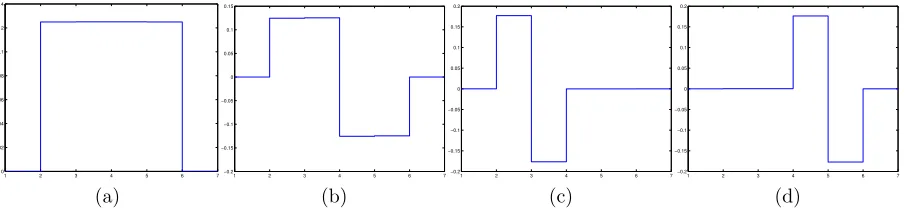
6.1 The staircase signal

We consider a simple example where the signals are binary, each consists of long sequences of +1’s separated by long sequences of −1’s, as shown in Figure 4. Let s

be the minimum length of consecutive +1 and−1 blocks. sis a measure of the lowest frequency of the signal. We use Algorithm 1 to learn the filters with η = 102_{. The}

filters learned are shown in Figure 5.

Figure 4: A binary signal

In the case whenm = 2, r= 2, we recover the Haar wavelet basis as shown Figure 6.

1 2 3 4 5 6 7 0 0.02 0.04 0.06 0.08 0.1 0.12 0.14 (a)

1 2 3 4 5 6 7 −0.2 −0.15 −0.1 −0.05 0 0.05 0.1 0.15 (b)

1 2 3 4 5 6 7 −0.2 −0.15 −0.1 −0.05 0 0.05 0.1 0.15 0.2 (c)

1 2 3 4 5 6 7 −0.2 −0.15 −0.1 −0.05 0 0.05 0.1 0.15 0.2 (d)

Figure 5: The filters learned using the parameters m= 4, r= 4, s= 30.

1 1.5 2 2.5 3 3.5 4 4.5 5 0 0.1 0.2 0.3 0.4 0.5 0.6 0.7 0.8 (a)

1 1.5 2 2.5 3 3.5 4 4.5 5

−0.8 −0.6 −0.4 −0.2 0 0.2 0.4 0.6 0.8 (b)

Figure 6: The filters learned using the parametersm = 2, r= 2, s= 30. In this case, we recover the Haar wavelets.

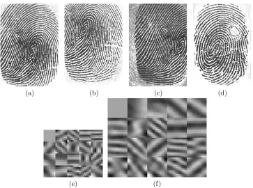
6.2 Fingerprint signal

Our next example is the fingerprint dataset (Maltoni et al., 2009). We use a fraction of the database. The input are 80 images of size 364×256. Some sample images and filters learned are shown in Figure 7. The filters are learned using Algorithm 2 with parameters η= 102, λ= 103. The main feature of the fingerprint images is that they contain oscillations along different directions. As can be seen from the Figure 7, this feature is indeed captured by the learned filters.

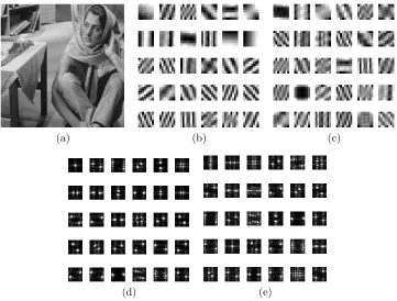
6.3 Another test image

The next example is a well-known natural image shown in Figure 8. This is an example of the redundant bi-frame case. We learn the decomposition filters using Algorithm 2 with η = 102_{, λ = 10}3_{. Note that some filters look like edge detectors}

(a) (b) (c) (d)

(e) (f)

Figure 7: (a)(b)(c)(d)Sample images of finger print.(e) Decomposition filters learned with support size 7×7. (f) Decomposition filters learned with support size 13×13.

7. Recover Predefined Wavelets

The proposed framework is an adaptive extension of the well-known wavelets and wavelet frames. It is natural to ask whether the standard wavelet filters can be recovered using this framework. Naturally we expect that if the signal has a sparse representation in a predefined wavelet domain, then the adaptive frames and bi-frames would recover the predefined wavelets.

To see whether this is the case, we generate the signals using linear combinations of different wavelets with different levels of sparsity. Specifically, the signals are gener-ated using 4 Daubechies wavelets of different support size, “db2”,“db3”,“db12”,“db24” in MATLAB syntax. Sparse random vectors with a given sparsity level are generated (the sparsity level is the ratio of the number of nonzeros coefficients to the length of the coefficient vector, we also call it the density), and these vectors are used as the coefficients of the signals under the wavelet transform.

Given a signal, the adaptive filters are learned by solving (17). Since (17) is nonconvex, to avoid complications coming from local minimum, we used the simulated annealing algorithm to perform the global optimization. We then compare the filters obtained with the original wavelets used to construct the signal. We declare success if the l2 norm of the difference between the adaptive filters and the predefined wavelets

(a) (b) (c)

(d) (e)

Figure 8: (a) Input image of size 512×512. (b) 30 decomposition filters with support size 8×8. (c) A specific set of reconstruction filters. (d) Fourier spectrum of the decomposition filters. (e) Fourier spectrum of the reconstruction filters.

Density db2 db3 db12 db24

0.1 1 1 1 1

0.2 1 1 1 1

0.3 1 1 1 1

0.4 1 1 0 0

0.5 0 0 0 0

Table 2: Ratio of successful recovery of predefined wavelets.

each case. The result is indeed consistent with our expectation. It is interesting to see that the transition is very sharp.

Figure 9 shows the adaptive filters for the case when the signals are generated using a dense combination of the predefined wavelets. In this case, the predefined wavelets are not optimal, and the signals have a sparser representation under the adaptive filters, as can be seen from Figure 9(c). The L1 norm of the wavelet coefficients is

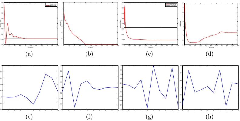
0 20 40 60 80 100 120 140 160 180 200 450 500 550 600 650 700 750 800 850 Iterations Function value Daubechies AdaFrame (a)

0 20 40 60 80 100 120 140 160 180 200

0 0.2 0.4 0.6 0.8 1 1.2 1.4 Difference Iterations (b)

0 100 200 300 400 500 600 700 800 900 1000 230 240 250 260 270 280 290 300 310 Iterations Function value AdaFrame Daubechies (c)

0 100 200 300 400 500 600 700 800 900 1000

1.1 1.15 1.2 1.25 1.3 1.35 1.4 1.45 1.5 1.55 Difference Iterations (d)

1 2 3 4 5 6 7 8 9 10

−0.4 −0.2 0 0.2 0.4 0.6 0.8 1 (e)

1 2 3 4 5 6 7 8 9 10

−0.8 −0.6 −0.4 −0.2 0 0.2 0.4 0.6 0.8 (f)

1 2 3 4 5 6 7 8 9 10

−0.5 −0.4 −0.3 −0.2 −0.1 0 0.1 0.2 0.3 0.4 0.5 (g)

1 2 3 4 5 6 7 8 9 10

−0.6 −0.4 −0.2 0 0.2 0.4 0.6 (h)

Figure 9: (a) The signal is generated using sparse linear combinations of the Daubechies wavelets. The black line is the objective function value evaluated us-ing the Daubechies wavelets, which is optimal in this case. The value below the black line is due to infeasible intermediate solutions. (b) The filters learned also converge to the Daubechies wavelets, the figure shows the difference of the adaptive filters and the Daubechies wavelets measured in Frobenius norm. (c) The signal is generated using a dense linear combinations of the Daubechies wavelets. In this case, the ob-jective function converges to a value lower than that of the the wavelets, indicated by the horizontal line. (d) The filters learned also converge, but to something different from the Daubechies wavelets. (e)(f) Decomposition filters of the Daubechies wavelet “db5”. The signal is generated using sparse linear combination of this wavelets, the filters learned are the same as the wavelets. (g)(h) The filters learned for signals generated using dense combinations of the “db5” wavelet. They are different from the wavelet filters.

8. Sample Applications

In this section, we discuss some examples of applications of the multi-scale adaptive frames, the AdaFrames. A thorough comparison of the proposed model and other existing models will be postponed to future publications.

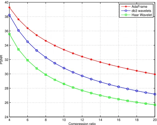
8.1 Image Compression

coars-est level to get the coefficients, but we keep only the coefficients with relatively large absolute values and set all the other coefficients to 0. The ratio of the total number of coefficients to the number of coefficients kept is called the “compression ratio” (the entropy coding stage is not considered here). We then perform a reconstruction step to get the reconstructed image ˆx. The quality of the compression is measured by the peak signal-to-noise ratio (PSNR). For monochrome 8 bit image, PSNR is defined as

PSNR(x,xˆ) = 10 log₁₀ 255

2 1

M N

PM

i=1

PN

j=1(ˆx(i, j)−x(i, j)2)

(41)

The filters are learned using image 8(a). 4 filters of support size 6×6 are learned using Algorithm 1 with η = 102_{. The coefficients are critically down-sampled with}

sampling matrix M = Diag(2,2). Initialization is done using the Daubechies filters db3. In general, we have found that using predefined wavelet frames as initialization works quite well. 7 levels of decompositions are performed using the architecture shown in Figure 2 and the same set of filters. The PSNR values are plotted against the “compression ratio” in Figure 10.

4 6 8 10 12 14 16 18 20

24 26 28 30 32 34 36 38 40

Compression ratio

PSNR

AdaFrame db3 wavelets Haar Wavelet

Figure 10: Image compression example. With the same image quality (measured in PSNR), AdaFrames achieves significantly higher compression ratio than the Haar wavelets and the Daubechies wavelets.

8.2 Image Denoising

(Buades et al., 2005), BM3D (Dabov et al., 2007), and the more recent ones based on dictionary learning (Elad and Aharon, 2006).

Among the various models, we select the K-SVD model (Elad and Aharon, 2006) as a benchmark for comparison since it is closely related to AdaFrames and since it has been shown to achieve the state of the art results.

Assume the image is corrupted by some additive noise:

g =f +n

where f is the clean image, g is our observation, and n is the noise with unknown distribution. First let us recall the procedure for wavelet domain denoising. Let WA

andRAbe the decomposition and reconstruction operators associated with the filters

A respectively. Given an observed image x, the denoised image is then given by:

ˆ

x=RA(shrink(WAx)) (42)

The procedure for AdaFrame denoising is exactly the same as that of wavelet domain denoising. Given the input image, we first learn the filters from the data using Algorithm 1 (or Algorithm 2 if we want to use bi-frames). We then use (42) to denoise.

In the first example, the input is a single image normalized to [0,1] and is corrupted with an additive Gaussian white noise with σ = 0.1. We train the filters both from the noisy image and the clean image with m = 36, r = 6, η = 102, λ = 103. A two-level decomposition is performed. The soft thresholding parameter is set to be 0.14. Initialization is done by setting the filters to be random orthogonal vectors. The result is shown in Figure 11. The performance of the K-SVD algorithm depends on the number of the atoms in the dictionary. Generally, the performance is better as we increase the number of atoms. In this example, 256 atoms with size 6×6 are used.

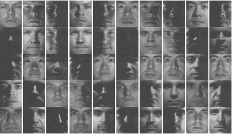
It is not surprising that the filters learned from a clean image produces better quality images: One can see from Figure 12 that the fine textures of the image are recovered. At a first sight, one might feel that this is impractical since we normally do not have access to the clean images. Nevertheless, there do exist realistic settings where learning from clean images makes sense. One such a situation is that filters learned from one set of clean images can then be used on another set of noisy images. We tested this idea on the extended Yale human face dataset B (Lee et al., 2005). It contains 16128 images of 28 human subjects. We used a subset of the images by picking the first 20 images of each of the subjects. We then added Gaussian white noise with σ = 0.1 to get the simulated noisy images. A glimpse of the dataset is in Figure 13.

(a) (b) (c) (d)

Figure 11: (a) Noisy input image, σ = 0.1. (b) K-SVD denoising re-sult, PSNR=28.65dB. (c) AdaFrame denoising, filters learned from noisy image, PSNR=28.8dB. (d) AdaFrame denoising, filters learned from the clean image, PSNR=29.3dB.

(a) (b) (c)

Figure 12: (a) Zoom in Figure 11(b). (b) Zoom in of Figure 11(c). (d) Zoom in of Figure 11(d).

K-SVD, noisy K-SVD, clean AdaFrame, noisy AdaFrame, clean

PSNR 31.4dB 32.01dB 31.35dB 32.07dB

Table 3: Average PSNR on the simulated noisy images on the extended Yale human face dataset B.

Figure 13: Simulated noisy images from extended Yale face dataset B

Test Image K-SVD 8×8 K-SVD 12×12 AdaFrame 8×8 AdaFrame 12×12

Barbara σ = 0.02 38.02 38.00 37.34 38.21

Barbara σ = 0.05 33.28 33.01 31.87 33.22

Barbara σ = 0.1 29.47 29.24 29.18 29.70

Boatσ = 0.02 37.02 36.71 36.75 36.86

Boatσ = 0.05 32.53 32.11 32.50 32.59

Boat σ= 0.1 29.19 28.70 29.18 29.21

House σ = 0.02 39.45 39.25 39.18 39.17

House σ = 0.05 35.12 34.74 34.50 34.66

House σ= 0.1 32.15 32.05 31.19 31.45

Lena σ= 0.02 38.45 38.21 37.98 38.45

Lena σ= 0.05 34.46 34.18 33.21 34.34

Lena σ = 0.1 31.38 30.84 31.12 31.39

Peppersσ = 0.02 37.68 37.47 37.30 37.46

Peppersσ = 0.05 33.94 33.52 33.32 33.79

Peppers σ= 0.1 31.26 30.78 30.33 30.91

Table 4: Comparison of AdaFrame and K-SVD, performance measured in PSNR, the unit is dB.

are learned. λ is chosen based on the noise level and is set to beλ= 0.005,0.01,0.025 respectively. The result is shown in Table 5.

As a last denoising example, we apply AdaFrames to some examples of natural photos with unknown noise. The setting is the same as the previous example. We learn filters directly from the noisy images. Since the image has RGB channels, we learn the filters (of support size 9×9) for each channel seperately with the same value of λ, which is chosen to yield a good visual impression. The results are shown in Figure 14.

(a) (b)

(c) (d)

Figure 14: (a)(c) Two images from the Internet. (b)(d) Denoised images using AdaFrame.

and the AdaFrame denoising algorithm. In our laptop with the same setup, the K-SVD algorithm takes 25s to train a dictionary with 256 atoms of support size 8×8 and 6.5s to denoise the image. The software we use is downloaded from http:// www.cs.technion.ac.il/~ronrubin/software. The AdaFrame takes 3.7s to train 64 filters with support size 8×8 and takes 0.6s to denoise. The time for denoising scales linearly with the number of filters.

8.3 Image Classification

Although AdaFrames are aimed to produce sparse representations, they can also be used to for other tasks such as extracting features for object recognition. In fact, it can provide a faster alternative to sparse coding.

AdaFrames. The results are sent to a linear support vector machine (SVM) to perform the classification task. We discuss three different set of experiments.

In the first setup, we use Algorithm 2 to learn the filters with m = 6, r = 6, η = 102, λ = 103. Initialization is done with random orthogonal filters. For each image, we perform a one-level decomposition to get the coefficients.

The second setup is identical to the first one, except m = 12 instead of m = 6. It is generally believed that lifting the raw pixels to some higher-dimensional feature space will be helpful for classification. Since we use more filters in this setup, the features we get have higher dimensions. Indeed the results are better than the results of the previous setup.

In the third setup, we use a two-level decomposition. We use Algorithm 2 to learn the filters with m = 6, r = 6, η = 102_{, λ = 10}3_{. Same nonlinear transformation as}

in the previous setups are used. In this way, we obtain 6 feature maps, each of size 28×28. Then the collection of the feature maps are treated as 6 sets of new input images. For each set, we use Algorithm 2 with m = 4, r = 6, η = 102_{, λ = 10}3 _to

learn the filters. Hence we have 24 filters in total. For each feature map, we perform a one-level decomposition using the corresponding 4 filters to get 4 feature maps. Again, we keep the positive coefficients and set the negative coefficients to 0. These positive coefficients in the first and second layers are the extracted features.

MNIST Raw pixel I II III

Precision 88.0 % 97.0 % 97.4% 99.0%

Table 5: Results of the MNIST classification. “Raw pixel” means that the features are the raw pixels.

These features are sent to a linear SVM. The results are reported in Table 5. Note that there is a significant reduction in the error rates compared to raw pixel features. As a point of comparison, the state-of-the-art result with preprocessing, is 0.23%, which is obtained using deep convolutional neural networks (Ciresan et al., 2012).

9. Connection with De-convolutional net

neighborhood of each node, is the most popular. It is similar to simple down-sampling but is nonlinear.

Although convolutional nets are designed for feature extraction and object recog-nition, it is an interesting question to ask how much of the input data can be re-constructed from the information in the intermediate layers of the network. For one thing, this can help us to gain some intuition about how convolutional nets work.

Figure 15: The left figure shows the typical structure of a convolutional layer from a convolutional net, the right figure shows the structure of a de-convolutional layer from a de-convolutional net.

In this regard the most popular approach in the literature is the “deconvolutional net” (Zeiler et al., 2010). A deconvolutional net can be thought of as a convolutional net that uses the same components (filtering, nonlinear activation, pooling) but in reverse order. Specifically a deconvolutional net consists of the following steps: First, the pooling procedure is reversed. If averaging or other linear operator is used for pooling, then to reverse it, one simply applies its transpose operator. The max-pooling procedure is a non-linear operation. For an image I, the max-pooling operation has two outputs, the maximum value and the position where the maximum value is obtained, defined as

(v, p)(x) = (sign(I(x))·max

x∈N |I(x)|,arg maxx∈N |I(x)|)

where N is the neighborhood of x. To reverse max-pooling, we set

I(x) =

v :x=p, x∈ N

0 :x6=p, x∈ N

their inverse. The situation where the activation function is non-invertible as is the case of the absolute value function is more complicated and is discussed in Wald-spurger et al. (2012).

The third component is to reverse the convolution operator, hence the name “de-convolution net”. Since “de-convolution is a linear operator, to reverse it, one applies its transpose (Zeiler and Fergus, 2013).

The above procedure is summarized in a diagram in Figure 15. Notice the sim-ilarity with applying wavelet frame transforms. A single level decomposition and reconstruction step of the wavelet frame transform can be described as in Figure 16. We see that if we ignore the point-wise nonlinearity, a convolutional or a deconvo-lutional layer is very similar to a decomposition and reconstruction step in wavelet bi-frame transform respectively.

Figure 16: One level decomposition and reconstruction of AdaFrame

There is a subtle but important difference. In deconvolutional net, deconvolution is done by applying the transpose of the convolution operator. In the one level wavelet bi-frame reconstruction, this is done using the reconstruction filters, obtained by solving (10), as required by UEP. Since there is no guarantee that the UEP condition is satisfied by the filters obtained in the convolutional nets, one expects that there will be errors in the reconstruction process, i.e. the deconvolutional nets. This is indeed the case, as we show below.

We implemented a two-layer convolutional network. In the first layer, we have 12 filters of support size 6 × 6, the pooling procedure is chosen to be the usual down-sampling with decimation factor (2,2). To construct the second layer, we stack together the feature maps from the first layer and form a three-dimensional signal. We then learn 12 filters of support size 4×4×2, the pooling procedure is also down-sampling with decimation factor (2,1,2). The activation function is the sigmoid function. The results of reconstructing the input image using the original deconvo-lutional net and the modified procedure described above are shown in Figure 17. As one can see, using the deconvolutional net approach, we gradually lose information as we ascend in the layers, while using the AdaFrame, we do not lose information.

(a) (b) (c)

(d) (e)

Figure 17: (a) The input image. (b) Reconstruction from the first layer activations using “deconvolutional net” approach. (c) Reconstruction from the second layer ac-tivations using the “deconvolutional net” approach. (d) Reconstruction from the first layer activations using the AdaFrame. (e) Reconstruction from the second layer activations using the AdaFrame.

In addition to near perfect reconstruction, AdaFrame has the potential to be used as an initialization method for the convolutional parts of a typical convolutional net. This is a direction for future research.

10. Conclusion

Predefined wavelets and dictionary learning have both been very successful in their own ways. In this paper, we have proposed a framework, the AdaFrame, that natu-rally combines the advantages of both. It is multi-scale and computationally efficient as pre-defined wavelets and wavelet frames, while being adaptive as in dictionary learning. Unlike dictionary learning, the proposed framework guarantees perfect re-construction, which is an appealing property in many signal processing tasks.

learning procedure is also easier, especially when the system is very redundant in which case the learning procedure can be carried out in two phases by learning the decomposition and reconstruction filters separately.

In addition to the examples given in this paper, we believe that the proposed framework can be useful in many other applications. It is not restricted to image processing, it can be used on time series, videos and even graphs. We will explore these applications in subsequent papers.

Another direction for future investigation is to use the proposed framework as feature extraction tools for machine learning tasks. Sparse coding has been popular for this purpose. But the proposed framework should be a promising alternative since it is more efficient and it has a multi-scale structure. It should be particularly appealing when the computation cost is the main bottleneck, as is the case in some real-time object recognition systems.

Acknowledgments

Appendix

Proof of Theorem 1

For convenience, we need the following lemma.

Lemma 2 Let M be d×d sampling matrix and a, b ∈ l2(Zd) be finitely supported

sequences. Then

\

Sbv(ξ) =|det(M)|vˆ(MTξ)ˆb(ξ) (43)

and

b

Ta(MTξ) = |det(M)|−1

X

ω∈ΩM

ˆ

v(ξ+ 2πω)ˆa(ξ+ 2πω) (44)

where

ˆ

a(ξ) := X

k∈Zd

a(k)e−ik·ξ

and

ΩM := [(MT)−1Zd]∩[0,1)d

Proof For a sequence v ∈l2(Zd),

d

Sbv(ξ) =

X

k∈_Zd

(Sbv)(k)e−ik·ξ

=|det(M)|X

k∈_Zd

X

j∈_Zd

v(j)b(k−M j)e−ik·ξ

=|det(M)|X

k∈Zd

b(k−M j)e−i(k−M j)·ξX

j

v(j)e−iM j·ξ

=|det(M)|ˆb(ξ)ˆv(MTξ).

(45)

Let ˆu(ξ) = P

k∈_Zdv(k)a(k−n), then ˆu(ξ) = ˆv(ξ)ˆa(ξ). By definition of Ta, we have

(Ta)(n) = u(M n). So

d

Tav(MTξ) =

X

n∈Zd

(Tav)(n)e−in·M

T_ξ

= X

n∈Zd

u(M n)e−kM n·ξ ₍₄₆₎

On the other hand,

X

ω∈ΩM

ˆ

u(ξ+ 2πω) = X

k∈Zd

X

ω∈ΩM

e−ik·(ξ+2πω)

= X

k∈_Zd

u(k)e−ik·ξ X

ω∈ΩM

e−ik·2πω.

(47)

If k ∈ M_Zd, then P

ω∈ΩM e

−ik·2πω _{= |det(M)|; if k ∈}

Zd/MZd,Pω∈ΩM e

−ik·2πω _{= 0,}

so we have

X

ω∈ΩM

ˆ

u(ξ+ 2πω) =|det(M)| X

k∈MZd

u(k)e−ik·ξ=|det(M)|X

n∈Zd

Combining this with (46), we get the desired result.

Lemma 3 Let M be d × d sampling matrix and al, bl, l = 1,· · · , m be m finitely supported sequences. Then

m

X

l=1

SblTalv =v, ∀v ∈l2(Z

d_{) (49)}

if and only if, for any ω ∈ΩM := [(MT)−1Zd]∩[0,1)d

m

X

l=1

ˆ

bl(ξ) ˆal(ξ+ 2πω) =δ(ω). (50)

Proof By definition of the decomposition and reconstruction operators Wa and Rb,

we have

RbWav = m

X

l=1

SblTalv. (51)

which is equivalent to

m

X

l=1

\

SblTalv(ξ) = ˆv(ξ),∀v (52)

By the above lemma, we have

ˆ

v(ξ) =

m

X

l=1

(S\blTalv)(ξ)

=

m

X

l=1

|det(M)|Td_alv(ξ)(MTξ) ˆb_l(ξ)

=

m

X

l=1

X

ω∈ΩM

ˆ

v(ξ+ 2πω) ˆbl(ξ)ˆal(ξ+ 2πω)

(53)

If (52) holds true, then

m

X

l=1

X

ω∈Ω

ˆ

v(ξ+ 2πω) ˆbl(ξ) ˆal(ξ+ 2πω) =

X

ω∈ΩM

ˆ

v(ξ+ 2πω)δ(ω) = ˆv(ξ). (54)

holds for all v ∈l2(Zd).

Conversely, if (51) is true, we can choosev that is close to aδ-function. LetB(ξ0)

be the open ball centered at ξ0 with radius . Fix ω0 ∈ ΩM and ξ0 ∈ Rd, we can

1. ˆv(ξ+ 2πω0) = 1, for all ξ∈B(ξ0).

2. ˆv(ξ+ 2πω) = 0, for all ξ ∈B(ξ0), ω ∈Ω/{ω0}.

3. supp(ˆv)⊂2πω0+B2(ξ0)

This is possible because the set Ω is discrete.

Hence, for ξ∈B(ξ0),

ˆ

v(ξ) =

m

X

l=1

X

ω∈ΩM

ˆ

v(ξ+ 2πω) ˆbl(ξ)ˆal(ξ+ 2πω)

=

m

X

l=1

ˆ

bl(ξ)ˆal(ξ+ 2πω0)

(55) Hence, m X l=1 ˆ

bl(ξ)ˆal(ξ+ 2πω0) =δ(ω)

for all ξ ∈B(ξ0), since ξ0 and ω0 are arbitrary, we obtain the desired result.

Proof of Theorem 1.

Proof We only need to establish that (10) is equivalent to (52).

δ(ω) =

m

X

l=1

X

k∈_Zd

bl(k)eik·ξ

X

n∈_Zd

al(n)e−in·(ξ+2πω)

=

m

X

l=1

X

k,n∈Zd

bl(k)al(n)ei(k−n)e−in·2πω

(56)

Denote by ΓM := (M[0,1)d)∩Zd, then we haveZd= ΓM+MZd, replacenbyM n+γ,

we can rewrite the above equation as

δ(ω) =

m

X

l=1

X

γ∈ΓM

X

k,n∈_Zd

bl(k)al(M n+γ)ei(k−M n−γ)·ξe−i(M n+γ)·2πω

=

m

X

l=1

X

γ∈ΓM

X

k,n∈_Zd

bl(k+M n+γ)al(M n+γ)eik·ξe−kγ·2πω

(57)

Note that (e−iγ·2πω₎

ω∈ΩM,γ∈ΓM is the Fourier matrix, and its inverse matrix is

|det(M)|−1_(eiγ·2πω₎

ω∈ΩM,γ∈ΓM. Therefore,

(

m

X

l=1

X

k,n∈_Zd

bl(k+M n+γ)al(M n+γ)eik·ξ)γ∈ΓM

=|det(M)|−1_(eiγ·2πω₎

ω∈ΩM,γ∈ΓM(δ(ω))ω∈Ω

=|det(M)|−1_{(1,1,· · · ,1)}T_.

Hence

m

X

l=1

X

k,n∈_Zd

bl(k+M n+γ)al(M n+γ)eik·ξ =|det(M)|−1, ∀γ (59)

taking inverse Fourier transform, we get the desired result.

References

Michal Aharon, Michael Elad, and Alfred Bruckstein. -svd: An algorithm for design-ing overcomplete dictionaries for sparse representation. Signal Processing, IEEE

Transactions on, 54(11):4311–4322, 2006.

Amir Beck and Marc Teboulle. A fast iterative shrinkage-thresholding algorithm for linear inverse problems. SIAM Journal on Imaging Sciences, 2(1):183–202, 2009.

Joan Bruna and St´ephane Mallat. Invariant scattering convolution networks. Pattern

Analysis and Machine Intelligence, IEEE Transactions on, 35(8):1872–1886, 2013.

Ori Bryt and Michael Elad. Compression of facial images using the k-svd algorithm.

Journal of Visual Communication and Image Representation, 19(4):270–282, 2008a.

Ori Bryt and Michael Elad. Improving the k-svd facial image compression using a linear deblocking method. In Electrical and Electronics Engineers in Israel, 2008.

IEEEI 2008. IEEE 25th Convention of, pages 533–537. IEEE, 2008b.

Antoni Buades, Bartomeu Coll, and J-M Morel. A non-local algorithm for image denoising. InComputer Vision and Pattern Recognition, 2005. CVPR 2005. IEEE

Computer Society Conference on, volume 2, pages 60–65. IEEE, 2005.

Jian-Feng Cai, Hui Ji, Zuowei Shen, and Gui-Bo Ye. Data-driven tight frame con-struction and image denoising. Applied and Computational Harmonic Analysis, 37 (1):89–105, 2014.

Emmanuel J Candes and David L Donoho. Curvelets: A surprisingly effective non-adaptive representation for objects with edges. Technical report, DTIC Document, 2000.

Dan Ciresan, Ueli Meier, and J¨urgen Schmidhuber. Multi-column deep neural networks for image classification. In Computer Vision and Pattern Recognition

(CVPR), 2012 IEEE Conference on, pages 3642–3649. IEEE, 2012.

Ronald R Coifman and Mauro Maggioni. Diffusion wavelets. Applied and

Kostadin Dabov, Alessandro Foi, Vladimir Katkovnik, and Karen Egiazarian. Image denoising by sparse 3-d transform-domain collaborative filtering.Image Processing,

IEEE Transactions on, 16(8):2080–2095, 2007.

Ingrid Daubechies, Bin Han, Amos Ron, and Zuowei Shen. Framelets: Mra-based constructions of wavelet frames. Applied and Computational Harmonic Analysis, 14(1):1–46, 2003.

Ingrid Daubechies, Michel Defrise, and Christine De Mol. An iterative thresholding algorithm for linear inverse problems with a sparsity constraint. Communications

on pure and applied mathematics, 57(11):1413–1457, 2004.

Minh N Do and Martin Vetterli. Contourlets: a new directional multiresolution image representation. InSignals, Systems and Computers, 2002. Conference Record of the

Thirty-Sixth Asilomar Conference on, volume 1, pages 497–501. IEEE, 2002.

Michael Elad and Michal Aharon. Image denoising via sparse and redundant repre-sentations over learned dictionaries. Image Processing, IEEE Transactions on, 15 (12):3736–3745, 2006.

Kjersti Engan, Sven Ole Aase, and J Hakon Husoy. Method of optimal directions for frame design. In Acoustics, Speech, and Signal Processing, 1999. Proceedings.,

1999 IEEE International Conference on, volume 5, pages 2443–2446. IEEE, 1999a.

Kjersti Engan, Sven Ole Aase, and JH Husoy. Frame based signal compression using method of optimal directions (mod). In Circuits and Systems, 1999. ISCAS’99.

Proceedings of the 1999 IEEE International Symposium on, volume 4, pages 1–4.

IEEE, 1999b.

Tom Goldstein and Stanley Osher. The split bregman method for l1-regularized problems. SIAM Journal on Imaging Sciences, 2(2):323–343, 2009.

John C Gower and Garmt B Dijksterhuis. Procrustes problems, volume 3. Oxford University Press Oxford, 2004.

Bin Han. Pairs of frequency-based nonhomogeneous dual wavelet frames in the dis-tribution space. Applied and Computational Harmonic Analysis, 29(3):330–353, 2010.

RA Horn and CR Johnson. Topics in matrix analysis, 1991. Cambridge University

Presss, Cambridge.

Kevin Jarrett, Koray Kavukcuoglu, M Ranzato, and Yann LeCun. What is the best multi-stage architecture for object recognition? In Computer Vision, 2009 IEEE

Alex Krizhevsky, Ilya Sutskever, and Geoffrey E Hinton. Imagenet classification with deep convolutional neural networks. In Advances in neural information processing

systems, pages 1097–1105, 2012.

Rongjie Lai and Stanley Osher. A splitting method for orthogonality constrained problems. Journal of Scientific Computing, 58(2):431–449, 2014.

Quoc V Le, Alexandre Karpenko, Jiquan Ngiam, and Andrew Y Ng. Ica with re-construction cost for efficient overcomplete feature learning. InAdvances in Neural

Information Processing Systems, pages 1017–1025, 2011.

Yann LeCun, L´eon Bottou, Yoshua Bengio, and Patrick Haffner. Gradient-based learning applied to document recognition. Proceedings of the IEEE, 86(11):2278– 2324, 1998.

Honglak Lee, Alexis Battle, Rajat Raina, and Andrew Y Ng. Efficient sparse coding algorithms. InAdvances in neural information processing systems, pages 801–808, 2006.

Honglak Lee, Roger Grosse, Rajesh Ranganath, and Andrew Y Ng. Convolutional deep belief networks for scalable unsupervised learning of hierarchical represen-tations. In Proceedings of the 26th Annual International Conference on Machine

Learning, pages 609–616. ACM, 2009.

Kuang-Chih Lee, Jeffrey Ho, and David Kriegman. Acquiring linear subspaces for face recognition under variable lighting.Pattern Analysis and Machine Intelligence,

IEEE Transactions on, 27(5):684–698, 2005.

Julien Mairal, Guillermo Sapiro, and Michael Elad. Learning multiscale sparse rep-resentations for image and video restoration. Technical report, DTIC Document, 2007.

Julien Mairal, Michael Elad, and Guillermo Sapiro. Sparse representation for color image restoration. Image Processing, IEEE Transactions on, 17(1):53–69, 2008.

Stephane G Mallat. Multiresolution approximations and wavelet orthonormal bases

of 2 (). Transactions of the American mathematical society, 315(1):69–87, 1989.

Davide Maltoni, Dario Maio, Anil K Jain, and Salil Prabhakar. Handbook of

finger-print recognition. springer, 2009.

Yves Meyer. Wavelets and operators, volume 1. Cambridge university press, 1995.

Stanley Osher, Martin Burger, Donald Goldfarb, Jinjun Xu, and Wotao Yin. An iter-ative regularization method for total variation-based image restoration. Multiscale

Modeling & Simulation, 4(2):460–489, 2005.

M Ranzato, Fu Jie Huang, Y-L Boureau, and Yann LeCun. Unsupervised learning of invariant feature hierarchies with applications to object recognition. InComputer

Vision and Pattern Recognition, 2007. CVPR’07. IEEE Conference on, pages 1–8.

IEEE, 2007.

Amos Ron and Zuowei Shen. Affine systems inl 2 (r d): The analysis of the analysis operator. Journal of Functional Analysis, 148(2):408–447, 1997.

Zuowei Shen. Wavelet frames and image restorations. In Proceedings of the

Interna-tional congress of Mathematicians, volume 4, pages 2834–2863, 2010.

Ir`ene Waldspurger, Alexandre dAspremont, and St´ephane Mallat. Phase recovery, maxcut and complex semidefinite programming.Mathematical Programming, pages 1–35, 2012.

Matthew D Zeiler and Rob Fergus. Visualizing and understanding convolutional neural networks. arXiv preprint arXiv:1311.2901, 2013.

Matthew D Zeiler, Dilip Krishnan, Graham W Taylor, and Robert Fergus. Decon-volutional networks. In Computer Vision and Pattern Recognition (CVPR), 2010