Efficient and Accurate Methods for Updating Generalized
Linear Models with Multiple Feature Additions
Amit Dhurandhar [email protected]
Marek Petrik [email protected]
IBM TJ Watson,
1101 Kitchawan Road, Yorktown Heights, NY 10598 USA
Editor:Charles Elkan
Abstract
In this paper, we propose an approach for learning regression models efficiently in an environment where multiple features and data-points are added incrementally in a multi-step process. At each multi-step, any finite number of features maybe added and hence, the setting is not amenable to low rank updates. We show that our approach is not only efficient and optimal for ordinary least squares, weighted least squares, generalized least squares and ridge regression, but also more generally for generalized linear models and lasso regression that use iterated re-weighted least squares for maximum likelihood estimation. Our approach instantiated to linear settings has close relations to the partitioned matrix inversion mechanism based on Schur’s complement. For arbitrary regression methods, even a relaxation of the approach is no worse than using the model from the previous step or using a model that learns on the additional features and optimizes the residual of the model at the previous step. Such problems are commonplace in complex manufacturing operations consisting of hundreds of steps, where multiple measurements are taken at each step to monitor the quality of the final product. Accurately predicting if the finished product will meet specifications at each or, at least, important intermediate steps can be extremely useful in enhancing productivity. We further validate our claims through experiments on synthetic and real industrial data sets.
Keywords: linear regression, logistic regressions, lasso, group lasso, feature selection, manufacturing
1. Introduction
together in groups called lots through hundreds of processing steps with thousands of mea-surements being accrued as the wafers reach the end. At this point, the quality of the wafers is determined by either checking their speed or power. It can be extremely useful if one could, at least at critical intermediate steps, provide an accurate estimate of the final speed so as to possibly take corrective actions or avoid further processing.
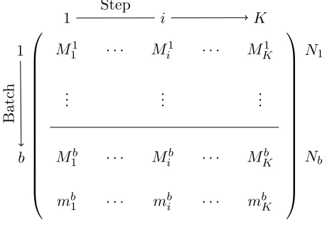
In particular, the data flows through K steps as groups of data-points or a batch with the target becoming available almost simultaneously for each member of the group at the very end. We want to efficiently build a model at each step based on this data so as to estimate the performance of forthcoming batches at these steps. There are multiple such batches that flow through the processing steps and hence, we also want to update our model at each step based on recently acquired data. Therefore, in our problem, both features and data-points are added as batches move through the process and as new batches are created. The notation used throughout the paper is given in Table 1 and an illustration of our problem setting is shown in Figure 1.
The methods we propose for incremental updates with new feature additions are by no means constrained only to manufacturing. They also are applicable to feature selection algorithms such as least angle regression (Efron et al., 2004), the homotopy method for lasso (Tibshirani and Taylor, 2011), or orthogonal matching pursuit (Hastie et al., 2009). These feature selection methods must efficiently update the model whenever a new feature is added. The most common approach is to keep a QR factorization of the regression matrix. This factorization can be updated with every new feature added using either Givens rotations or Householder reflections, which are both computationally efficient and numerically stable (Golub and Loan, 1996).
The problem we study differs from the typical feature selection setting in two important aspects. First, while most feature selection methods add one feature at a time, our method is more suitable when many features are to be added at a time. Second, the QR factorization can only be used with linear regressors, while our method also works with generalized linear models. As a result, our methods can also be applied in more sophisticated settings, such as to efficiently update regression models in non-linear group variable selection techniques (Lozano et al., 2009, 2011).
Our method when instantiated to the linear regression case, where we minimize a least squares objective, is closely related to the partitioned matrix inverse mechanism based on Schur’s complement (Boyd and Vandenberghe, 2004). Although both absolve the need for computing matrix inverses over the entire currently available feature set, our procedure has an intuitive explanation. Moreover, our method is a meta-technique applicable to any base regression method, and as you will see later, is an essential component in optimally updating generalized linear models such as logistic regression, which as we know are non-linear.
Term/Symbol Description
Step/Epoch The instant when new features become available. Batch A set of data points that move through all the steps.
di Number of features accumulated till (and including) stepi. Xb
i,xbi Input data from batchbwithdi and (di−di−1) features respectively.
Mb
i,mbi Model built on the firstdi features with all the data till batch b and only data in batchb respectively.
Yb Outputs corresponding to batchb. ˆ
Yqp,Rpq Matrix of predictions and the matrix of residuals respectively, obtained by regressing inputsqon columns ofp.
Table 1: The notation used in the paper. In much of the paper we drop the batch b from the superscript since, we propose methods for efficient updates to models with feature additions that are applicable to any batch.
M11 · · · Mi1 · · · MK1
..
. ... ...
M1b · · · Mib · · · MKb mb1 · · · mbi · · · mbK
1 Step i K
1 b Batc h N1 Nb
Figure 1: Process where features and data-points are added, with new models being learned at each step.
2. Problem Statement
Before describing the problem statement, we will introduce some notation. Let K denote the number of steps in the process. Letdi denote the number of featuresFi ={f1, ..., fdi}
present at step i. It is important to note that Fi ⊃ Fi−1,∀i ∈ {2, ..., K} which implies
di > di−1,∀i ∈ {2, ..., K}. There are multiple batches that flow through the K steps and we denote the size of one such batch b, by Nb. Based on a particular learning algorithm,
we denote the model learned at step i trained on data from batch b, bymbi (local model). LetMib (global model) denote the model based on all the data accumulated till batch bin step i. For efficiency reasons, though we may not learn from scratch in stepi using all the available data,Mib is obtained by potentially learning over a sample of sizePb
mbi is a local model learned over just recent data, while Mib is the model we will use to predict the outcomes of the data points in the (b+ 1)thbatch when they reach step i. Note that for batch 1, the local and global models are the same, i.e., m1i =Mi1,∀i∈ {1, ..., K}. A pictorial representation of the process with notation is shown in Figure 1.
Let Xib (Nb×di matrix) and xib (Nb ×(di−di−1) matrix) denote all the input data
available1 in step i batch b and the input data for only the additional features in step
i batch b, i.e., {fdi−1+1, ..., fdi} respectively. Let Yb denote the final outcomes or target
in batch b. Let ˆYqp and Rpq denote the matrix of predictions and the matrix of residuals
respectively, obtained by regressing inputsq on columns of p based on a chosen regression technique. Thus, ifpis a matrix, each of its columns is considered a target andqis regressed separately on each of them. Consequently, ˆYXYb
i
and RYXb i
are the predictions and residuals
of the modelmbi respectively. Let Ij denote an identity matrix of rank j.
Given our dual goal of efficiently learning with i) new features and ii) with new data points being added, we address each of these issues in isolation. With this, we have the following two problems that we need to tackle:
I During any batchbof theKstep process, given a model at stepi∈ {1, ..., K−1}learned overdifeatures{f1, ..., fdi}and a sample sizeNb, how do we update this model at step i+ 1 with di+1 features {f1, ..., fdi, ..., fdi+1} such that the resultant model is (a) no
less accurate than the model at stepi? (b) no less accurate than the composite model which consists of the model learned using only the additional features{fdi+1, ..., fdi+1}
on the residuals of the model at step i? and (c) more efficient to learn than learning from scratch over all the features available at stepi+ 1 i.e., {f1, ..., fdi+1}?
II At any stepiin theK step process, given the modelMib and the modelmbi+1, how do we efficiently obtain the modelMib+1?
Though not completely solved, there has been extensive work to handle Question II (Blum, 1996; Smale and Yao, 2005; Bottou and Cun, 2003). We thus focus our attention on question I. Given this and for simplicity of notation, from here on, we do not refer to the batch any more; that is, we drop b from the notation, since the methods we describe are applicable to any batch in the process.
3. Methodology
In this section, we first suggest a meta-algorithm to successfully tackle question I. We then show that not only can this algorithm be realized efficiently for ordinary least squares, weighted least squares, generalized least squares and ridge regression, but it is also optimal for these techniques. We also show that the algorithm can be used as a core function to efficiently and optimally solve iterated re-weighted least squares procedures, which are used to find the maximum likelihood estimates for Generalized Linear Models (McCullagh and Nelder, 1990) and sometimes even Lasso (Tibshirani, 1994). For arbitrary regression algorithms, it can be shown that even a relaxation of our technique results in a positive response to questions I(a), I(b) and I(c). We refer to the optimal model in any step that
Algorithm 1 Proposed meta-algorithm—which can be embedded as a core function in other algorithms—to update model built in step iduring the next step i+ 1. ζi are other
regression algorithm specific parameters. Input: mi,RYXi,Xi+1,Y and ζi.
Output: mi+1,RYXi+1 and ζi+1
Compute Rxi+1Xi {UseXi to predict columns ofxi+1 and compute the residual matrix.} RegressRxi+1Xi onRYXi →m¯i+1 {Regressing the residuals outputs the model on the right.} RegressXionY−Yˆ
RY Xi
RXixi+1 →mˆi{Regressing the input of stepiwith the previous residual
yields the model on the right.}
mi+1 = ( ˆmi; ¯mi+1) {Composing these models, i.e., for example concatenating their
pa-rameter vectors, gives the final model.}
if i+ 1 ==K then
{Ifi+ 1 is the last step.}
Returnmi+1 else
Returnmi+1,RYXi+1 and ζi+1 end if
is learned from scratch by method Standard. We refer to the model that learns on the additional features and optimizes the residue of a model at the previous step by method AFOR.
Algorithm 1 can be described as follows: First, we find the portion of the target that was not modeled by the regression algorithm (residuals) in the previous step. We then try to find the additional information that the new features in the current step contain. Using this additional information we fit to the residuals in the previous step. The residuals from this model are subtracted from the original target and the features in the previous step are fit to this modified target. The final model is a composition of these two latter models.
Loosely speaking, the intuition behind Algorithm 1 is to find what additional benefit the new features bring us in predicting the portion of the target that was not modeled by the previously available set of features, and after the removal of their effect, we focus on modeling this new modified target using the previously available set of features. This procedure thus uses the old and new set of features to model, as much as possible, the parts of the target that are not explained by the other, resulting in significantly reduced redundancy in the final model.
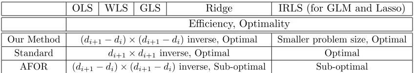
OLS WLS GLS Ridge IRLS (for GLM and Lasso) Efficiency, Optimality
Our Method (di+1−di)×(di+1−di) inverse, Optimal Smaller problem size, Optimal Standard di+1×di+1 inverse, Optimal Optimal
AFOR (di+1−di)×(di+1−di) inverse, Sub-optimal Sub-optimal
Table 2: Comparison of three meta-approaches across different regression algorithms in step
i+ 1. Standard denotes learning from scratch.
3.1 Generalized Least Squares and Ridge Regression
In least squares regression (Hastie et al., 2009), we minimize a quadratic loss function wherein each datapoint may be weighted or unweighted (i.e., equi-weighted). Based on the weighting scheme, we have the following three variants with each successive variant being a generalization of the ones before. Ordinary Least Squares (OLS) is the unweighted variant. Weighted Least Squares (WLS) is the variant, where the weight matrix is diagonal. Gener-alized Least Squares (GLS) is the most general variant, wherein we have a full weight matrix
W. Ridge regression on the other hand is regularized OLS with a quadratic penalty (Hoerl and Kennard, 1970).
We now instantiate Algorithm 1 for GLS with a quadratic penalty. We could refer to this method as Generalized Ridge (GR) regression. Eliminating the penalty term or setting
W to the identity matrix in GR would give us instantiations for GLS and ridge regression respectively.
The objective function minimized in stepi for GR is
Qgr = (Y −Xiβi)TW(Y −Xiβi) +λβiTβi,
where βi is the parameter vector we wish to estimate2 and λ > 0 is the regularization
parameter. The optimal βi is given by mi = (XiTW Xi +λIdi)−1XiTW Y, where Idi is a di×di identity matrix. To estimateβi+1 we use Algorithm 1 as follows:
• Rxi+1Xi = (IN −Hi)xi+1. Here ζi=Hi =Xi(XiTW Xi+λIdi)−1XiTW.
• m¯i+1= (xi+1TW(IN−Hi)xi+1+λI(di+1−di))−1xi+1T(IN−Hi)Y. This is a consequence
of the fact thatHi is idempotent.
• mˆi = (XiTW Xi+λIdi)−1XiTW(Y−xi+1m¯i+1) =mi−αim¯i+1, whereαi = (XiTW Xi+ λIdi)−1XiTW xi+1.
• mi+1= ( ˆmi; ¯mi+1). Nowmi+1 can be immediately used to obtain predictions for new batches whose target is currently unknown and have reached stepi+ 1.
• If i+ 1 < K, then return mi+1, RXi+1Y and Hi+1. Here Hi+1—which also deter-mines (Xi+1TW Xi+1+λIdi+1)−1—can be computed from (XiTW Xi+λIdi)−1 and
(xi+1TW(IN −Hi)xi+1+λI(di+1−di))−1 using standard partitioned matrix inversion property with only matrix multiplications but no more inversions (Boyd and Vanden-berghe, 2004).
Let us now see why this method is more efficient than performing regression from scratch in stepi+1. If we performed regression from scratch we would have had to invert adi+1×di+1 matrix. In our case however, we have to invert only a (di+1−di)×(di+1−di) matrix in
step i+ 1. The reason for this is that (XiTW Xi +λIdi)−1, which is a di ×di matrix, is
already available from step i. Moreover, our method is also more efficient at obtaining the current step model than applying the partitioned matrix inversion property based on Schur’s complement directly, because although no more inversions are required by it there are many more matrix multiplications that have to be performed.
For instance, based on Schur’s complement and the partitioned matrix inversion mech-anism we would compute the optimal estimate forβi+1 denoted by βiopt+1 as follows
βiopt+1=
XiTW Xi+λIdi XiTW xi+1
xTi+1W Xi xTi+1W xi+1+λI(di+1−di) −1
XiT xTi+1
Y
=
A−1+A−1U C−1V A−1 −A−1U C−1
−C−1V A−1 C−1
XiT xTi+1
Y
, (1)
whereA=XiTW Xi+λIdi,U =XiTW xi+1,V =xTi+1W XiandC=xTi+1W(IN−Hi)xi+1+
λI(di+1−di). HereC is the Schur’s complement.
It turns out that our estimate mi+1 = βiopt+1 and is thus optimal for GR regression as seen below.
Theorem 1 If we use GR regression in our process, then in any step i+ 1, where i ∈
1, ..., K−1,mi+1 is the optimal GR estimator.
Proof Equation (1) can be expanded and rewritten as follows
βiopt+1 =
A−1+A−1XiTW xi+1C−1xTi+1W XiA−1 −A−1XiTW xi+1C−1
−C−1xTi+1W XiA−1 C−1
XiT xTi+1
Y
=
A−1XiTW(Y −A−1XiTW xi+1TC−1xi+1T(IN−Hi)Y) C−1xi+1T(IN −Hi)Y
=
(XiTW Xi+λIdi)−1XiTW(Y −xi+1m¯i+1) (xi+1TW(IN −Hi)xi+1+λI(di+1−di))−1xi+1T(IN−Hi)Y
=
ˆ
mi
¯
mi+1
=mi+1
.
Remark 1 The result in Theorem 1 implies that using Algorithm 1, we get efficient and
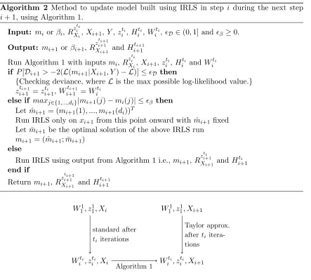
Algorithm 2 Method to update model built using IRLS in step i during the next step
i+ 1, using Algorithm 1.
Input: mi orβi,R ziti
Xi,Xi+1,Y,z ti i ,H
ti i ,W
ti
i ,D ∈(0,1] andβ ≥0.
Output: mi+1 orβi+1,R zi+1ti+1
Xi+1 andH
ti+1 i+1 Run Algorithm 1 with inputs mi,R
ztii
Xi,Xi+1,z ti i ,H
ti
i and W
ti i
if P[Di+1>−2(L(mi+1|Xi+1, Y)− L)]≤D then
{Checking deviance, where Lis the max possible log-likelihood value.}
ziti+1+1 =ziti+1,Witi+1+1 =Witi
else if maxj∈{1,...,di}|mi+1(j)−mi(j)| ≤β then
Let ˆmi+1= (mi+1(1), ..., mi+1(di))T
Run IRLS only onxi+1 from this point onward with ˆmi+1 fixed Let ¯mi+1 be the optimal solution of the above IRLS run
mi+1 = ( ˆmi+1; ¯mi+1)
else
Run IRLS using output from Algorithm 1 i.e., mi+1,R ztii+1
Xi+1 and H
ti i+1 end if
Return mi+1,R
zi+1ti+1
Xi+1 andH
ti+1 i+1
W11, z11, Xi W11, z11, Xi+1
Witi, ziti, Xi Witi, ztii , Xi+1 standard after
ti iterations
Algorithm 1
Taylor approx. afterti itera-tions
Figure 2: The figure shows where Algorithm 1 can be used to efficiently transform the optimal solution in stepito a solution in step i+ 1.
3.2 Generalized Linear Models and Lasso using IRLS
Generalized Linear Models (GLMs) assume that the target is generated from certain specific distributions belonging to the exponential family. Normal, Poisson, binomial, gamma and exponential are some of the distributions that are considered. The target is related to a linear combination of the inputs through a linear or non-linear function called the link function. Formally, if we learned a GLM in stepi, we would have the following relationship
E[Y] = ˆYXiY =g−1(Xiβi),
Lasso (Tibshirani, 1994) is L1 regularized OLS. It is usually used to solve under-determined systems of equations, where we have more features than data points. The idea here is to avoid over-fitting and choose features that are truly predictive. Formally, a lasso in stepiwould minimize the following objective
QL= (Y −Xiβi)T(Y −Xiβi) +λ|βi|1. 3.2.1 Iteratively Re-weighted Least Squares
Both of the above classes of regression methods can be solved using iterative procedures. Iteratively Re-weighted Least Squares (IRLS) is a popular technique used to find the max-imum likelihood estimates (MLE) for GLMs. Although there are other preferred methods to solve lasso, IRLS is still an effective method in this context. IRLS usually uses Newton Raphson updates, where the updated predictions at each iteration determine the weight matrix and the target in the next iteration. In particular, if Witj and zitj are the weight matrix and target in step i, and in the tthj iteration respectively, then the weight matrix is a N ×N diagonal matrix whose diagonal elements correspond to the reciprocal of the variances computed from predictions in the previous iteration (tj −1). z
tj
i on the other
hand is given by Xiβ tj−1
i +W
tj
i (Y −Yˆ zitj−1
Xi ).
On the left hand portion of Figure 2, we see that in step i if we run IRLS, we get the optimal solution after ti iterations. This optimal solution corresponds to an optimal
weight matrix Witi and an optimal target zitj. Using this weight matrix and target we can efficiently obtain the corresponding WLS solution in step i+ 1 using Algorithm 1. This solution relates to performing IRLS in step i+ 1, where at each iteration we approximate (zeroth order) the predictions aroundRXixi+1xi+1 using Taylor expansion
ˆ
Yz tj i+1 Xi+1 = ˆY
zitj
Xi +R
xi+1
Xi xi+1s(Xi+1, z
tj i+1),
where s(.) is a function denoting higher order terms. Hence, at each iteration if we take the zeroth order approximation, then the WLS problem solved has the same weight matrix and target as that solved in stepiat the same iteration. This is depicted on the right hand side of Figure 2.
3.2.2 Understanding Algorithm 2
In Algorithm 2, we first use Algorithm 1 to find the optimal solution in the current step
i+ 1 of the WLS problem at iteration ti in step i. The weight matrix and target in this
WLS problem correspond to the optimal IRLS solution in step i. We then check to see if the probability of deviance Di+1 (McCullagh and Nelder, 1990) being greater than twice the difference between the max possible log-likelihood value (i.e., if ˆYXi+1Y = Y) and the log-likelihood of the current solution is less than a small constantD. Deviance is a statistic
that measures goodness of fit. For any stepi,Di =−2(L(mi|Xi, Y)− L), wheremi denotes
a corresponding optimal model. Asymptotically, Di has a χ2 distribution with N −di
If this condition is not satisfied, we then check to see what is the maximum change in the
di parameter values going from the optimal IRLS solution in step ito our current solution
in step i+ 1. If the maximum change is small, i.e.,≤β, we fix these parameters and only
run IRLS on the remaining set. A small change in the previous step parameters indicates that the new set of features in step i+ 1 are practically orthogonal to step i features and hence, the previous step parameters will change little as we approach the optimal solution in the current step.
If neither of the above conditions are satisfied we simply run IRLS, starting at the current solution.
3.2.3 Analysis
It is easy to see that if the first condition in Algorithm 2 is satisfied, then we have reached our desired solution and hence, this is definitely more efficient than starting from the beginning. The question is, are we doing better in the other two cases, namely, when only the second condition is satisfied or when neither condition is satisfied? The latter scenario is probably worse since, we are solving at each iteration a WLS problem withdi+1 features rather than
di+1−di features. We cannot claim for certain that these two scenarios are more efficient
than learning afresh in stepi+ 1, but the following two results along with experiments on real industrial data lead us to strongly believe that this is the case.
As the log-likelihood of the predictions increases after each iteration in step i, the vari-ances and hence, the weight matrix approach the true weight matrix. Hence, the optimal weight matrix in step i represents the variances much more accurately than starting with the default, which is uniform weights.
Remark 2 Using the optimal weight matrix and target of step ias a starting point for step
i+ 1 has a higher log-likelihood solution than starting with the defaults, i.e., uniform weight
matrix and the original target (Pregibon, 1981; Wang, 1987; McCullagh and Nelder, 1990).
Based on Remark 2, one might ask, does starting from a higher likelihood point guar-antee us faster convergence or fewer iterations? Loosely speaking, in the proposition that follows, we show that better initialization leads to no worse a solution after the same number of iterations.
Proposition 1 When using IRLS, if two feasible points β1 and β2 are in the neighborhood
of the same local optimum γ of a log-likelihood function where the Hessians exist and the
first partial derivatives are non-zero, with L(β1|X, Y) ≥ L(β2|X, Y), then a tight upper
bound on the distance of the solutions starting at each of these points to γ aftert iterations
has the following relationship, ηt(β1)≤ηt(β2), where ηt(.) is a function that takes as input
the starting point and outputs the required upper bound on the distance at iteration t.
Proof Let γ be the root of the log-likelihood function L(.). The log-likelihood is always conditioned on inputs and outputs but for notational conciseness we do not repeatedly write this here. Let βjt denote the solution of IRLS at iteration tstarting from the initial point
βj. Thus, by Taylor expansion starting from β1 at iteration twe have
L(γ) =L(β1t) +5L(β1t)T(γ−β1t) +1 2(γ−β
t
where 5 denotes the gradient and F(.) denotes the hessian. Since, γ is the root of the above function and after pre-multiplying by the inverse of the Jacobian at β1t we have
γ−β1t+J−1(β1t)L(β1t) =−1
2J
−1(βt
1)(γ−βtj)TF(β1t)(γ−β1t)
γ−β1t+1=−1
2J
−1(βt
1)(γ−βjt)TF(β1t)(γ−βt1)
,
since, β1t+1 =β1t−J−1(β1t)L(β1t). Now if we take norm on both sides we get
|γ−β1t+1|= 1 2|J
−1(βt
1)F(β1t)||γ−β1t|2. Let ∆t1 =|γ−β1t|. Thus
∆t1+1= 1 2|J
−1(βt
1)F(β1t)|∆t1 2
.
Let Nj denote the neighborhood around γ such that Nj = {β|L(β) ≥ L(βj)}. Let uj =supβ∈Nj
1 2|J
−1(β)F(β)|. We thus have
∆t1+1 ≤u1∆t12
≤ut1∆112 =ηt+1(β1)
,
whereηt+1(β1) =ut1∆11 2
. Similarly, if we started atβ2 we would have ∆t2+1 ≤ηt+1(β2).
Now if L(β1) ≥ L(β2), thenN1 ⊂ N2 and hence, u1 ≤u2. Moreover, ∆11 ≤∆12. Based on these two facts we would have
ηt+1(β1)≤ηt+1(β2).
The assumptions in Proposition 1 about local Hessians and the Jacobian matrix are stan-dard assumptions used in proving convergence of Newton-Raphson’s method (Luenberger, 1984). These are not additional assumptions that we make.
Based on Remark 2 and Proposition 1, we can say that starting from the optimal weight matrix and target of the previous stepiwill lead to fewer iterations in the current stepi+ 1, which means faster convergence.
3.3 Other Regression Techniques
In the previous sections, we showed that using Algorithm 1 just by itself or using it as a core function in other algorithms can lead to optimally and efficiently solving regression problems that use a rich class of regression techniques. This naturally implies that questions I(a), I(b) and I(c) in Section 2 have been answered positively for these cases. In this section, we try to answer these questions for arbitrary linear or non-linear regression algorithms.
If we again use Algorithm 1 for an arbitrary regression algorithm, it may very well provide accurate predictions but is likely to be inefficient. The most expensive computation in Algorithm 1 would be computing the residual of fittingXi onto each column ofxi+1. This
could potentially lead to running the chosen regression algorithmdi+1−di times. We want
to save on these computations and therefore, we relax Algorithm 1, where we simply fit
xi+1 toRYXi rather than fitting R xi+1
Xi toRYXi. Let us refer to this new version of Algorithm
1 by Algorithm 1(r). Let us now see if Algorithm 1(r) also results in a positive response to questions I(a), I(b) and I(c).
Let us denote the error or residual of the optimal model built in step i (previous step) by δprev. If AFOR optimizes the residual of this model—which leads to the best AFOR
model—based on xi+1, then we denote its error by δAF ORbst . Let the error of our relaxed
method be denoted byδ1(r). With this, we have the following result,
Proposition 2 Algorithm 1(r) in step i+ 1 is no less accurate than the model in stepiand AF OR in step i+ 1, i.e., δ1(r) ≤δbstAF OR≤δprev.
Proof We have δprev = RYXi and δAF ORbst = R RY
Xi
xi+1. Thus, δAF ORbst can be written as, δAF ORbst = Rδprevxi+1. Since in AFOR we optimize the residual of the model at the previous
step, we have
δprev≥δAF ORbst .
In our relaxed method, we first fit xi+1 toRYXi. We then fit Xi to Y(r) =Y −Yˆ RY
Xi xi+1 and
whose error maybe denoted by δ1(r) =RY (r)
Xi . Thus,δ1(r) can be written as,δ1(r) =R δbst
AF OR Xi
and since we optimize the residual of AFOR we have
δAF ORbst ≥δ1(r).
Proposition 2 implies a positive response to questions I(a) and I(b). It is also easy to see that Algorithm 1(r) is more efficient than learning over the whole space and hence, we also have a positive response for I(c). If we further relax Algorithm 1 to exclude fittingXi
toY(r), then our method is reduced to AFOR.
4. Addressing Question II
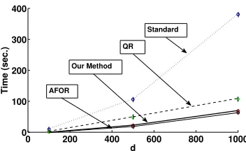
0 200 400 600 800 1000 0
100 200 300 400
d
Time (sec.) AFOR Our Method
Standard
QR
Figure 3: Total training time for OLS summed over the three steps for the different methods with different number of featuresdadded at each step.
There are numerous works in online learning (Blum, 1996; Smale and Yao, 2005; Bottou and Cun, 2003), where existing models are updated using stochastic techniques in time proportional to the newly added information. A common update procedure for many para-metric models is to perform additive updates. Thus, in step i and based on the data up until batchb, if we have a modelMi and we learn a model based on batchb+ 1,mbi+1, then
the model based on data up until batch b+ 1 would be given by
Mib+1=Mib+ν(mbi+1−Mib),
whereνb ∈[0,1] is the learning rate when batchb+ 1 becomes available. It is reasonable to makeνb a function ofNb+1 andS=Pbj=1Nj, where the learning rate is higher whenmbi+1
is obtained by learning over a relatively larger data set. For example, νb = Nb+1
Sb+1. Other
possible updates are multiplicative updates (Arora et al., 2005), where the original model
Mib can be updated based on its error in relation to the error of mbi+1.
5. Experiments
In this section, we empirically validate our claims through synthetic and real data experi-ments.
5.1 Synthetic Experiments
We consider the setting where we have three feature subsets or steps (i.e., K = 3) each of d dimensions. We generate data from a 3d+ 1 dimensional Gaussian, where the firstd
dimensions make up the first representationX1, the nextdmake up the next representation
0 200 400 600 800 1000 −2.6
−2.4 −2.2 −2 −1.8 −1.6 −1.4 −1.2x 10
5
d Log−likelihood AFOR
Our Method, Standard, QR
Figure 4: Average log-likelihood of the final model for the different methods with different number of featuresdadded at each step for OLS.
0 200 400 600 800 1000
0 200 400 600 800
d Time (sec.) AFOR
Our Method
Standard
WS
Figure 5: Total training time summed over the three steps for the different methods with different number of featuresdadded at each step for logistic regression.
0 200 400 600 800 1000
−12 −10 −8 −6
−4x 10
4
d
Log−likelihood
AFOR
Our Method, Standard, WS
correlation matrix and the mean set to zero we generate 100 data sets of 10000 points for each of the three values of d, namely: a) d= 100, b)d= 500 and c) d= 1000.
We compare the performance of our algorithms with a) learning from scratch i.e., stan-dard, b) AFOR and c) QR decomposition based updates using Givens rotations (Stewart, 2001; Golub and Loan, 1996) or warm starting (QR and WS), for two regression methods namely, OLS regression and logistic regression (β =D = 0.1). QR decomposition
(Stew-art, 2001) is only efficient in the OLS case since for logistic regression we have to perform the decomposition—not simply update—at every step as the optimal weight matrix and target keep changing. Thus, we use QR only for OLS, while warm starts are only applicable for logistic regression. For logistic regression, we discretize the target where we insert a value of 1 if the target has value ≥ 0, otherwise we insert a 0. We perform 10-fold cross validation and report the total training time summed over the three steps and the average test likelihood of the final model for each value ofdwith a 95% confidence interval.
In Figure 3, we see that the standard method takes significantly more time than the other methods. Our method is almost as fast as AFOR which is very promising and much faster than QR based updates. The performance gain of our method compared to the other optimal methods improves as d increases. In Figure 4, we see that AFOR is significantly worse in terms of accuracy than the other methods which are all optimal. In Figure 5, we see a similar trend as in the OLS case. However, the speedup of our method is greater and for the case with the highest d, our method is even faster than AFOR. A possible reason for this is that in one or more steps the updating using Algorithm 1 is much better than starting from the default even with just the added features. Here again, as seen in Figure 6, AFOR has much lower accuracy than the other methods that are optimal.
5.2 Real Data Experiments
We evaluate our methods on two real industrial data sets obtained from diverse domains. The first experiment is on a chip production data set obtained from the semiconductor industry. In this empirical study we compare the different updating strategies mentioned in this paper to learn a regression model. In the second experiment, we consider a finance data set, where we want to find which sources of information (or feature sets) are predictive of the final revenue. In this case, we run LogitGOMP (Lozano et al., 2011) to select the feature sets. When a feature set is selected, we update the current model using the different updating strategies. We then compare the runs of LogitGOMP based on these different strategies. Through this experiment we show that our method can also be effectively used to speed up sophisticated group variable selection techniques in real world settings. In both the experiments we add another straw man, which learns only on the features available at the particular step. We refer to this method, which learns only on the additionalfeatures as AF.
5.3 Regression in Chip Manufacturing
1 2 3 82
84 86 88 90 92 94
Step
Test Accuracy
Our Method, Standard, QR
AFOR
AF
Figure 7: Test set accuracy of the methods in classifying wafers as in spec or out of spec at the respective steps for OLS.
77
1 2 3
80 85 90 95 100
Step
Test Accuracy
AF
AFOR Our Method, Standard, WS
Figure 8: Test set accuracy of the methods in classifying wafers as in spec or out of spec at the respective steps for logistic regression.
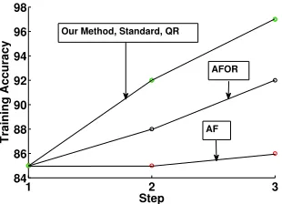
1 2 3
84 86 88 90 92 94 96 98
Step
Training Accuracy
Our Method, Standard, QR
AFOR
AF
Step 2 Step 3
Time Ltr(.) Ltst(.) Time Ltr(.) Ltst(.)
Our Method 20.6 -1991.8 -2156.2 17.8 -1742.1 -1895.5 Standard 100.1 -1991.8 -2156.2 145.9 -1742.1 -1895.5 AFOR 20.4 -2693.4 -3482.5 17.5 -2176.7 -3285.2 AF 20.2 -3793.7 -4755.5 17.4 -3893.7 -4712.3 QR 72.3 -1991.8 -2156.2 67.5 -1742.1 -1895.5
Table 3: Average time (in sec.) the least squares methods take to train in each of the steps, the average training log-likelihood value Ltr(.) in the respective steps and the average test log-likelihood valueLtst(.) in the respective steps.
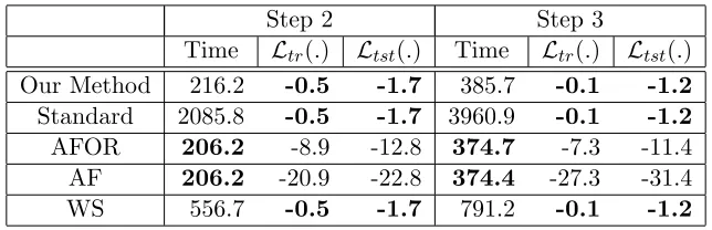
Step 2 Step 3
Time Ltr(.) Ltst(.) Time Ltr(.) Ltst(.) Our Method 216.2 -0.5 -1.7 385.7 -0.1 -1.2 Standard 2085.8 -0.5 -1.7 3960.9 -0.1 -1.2
AFOR 206.2 -8.9 -12.8 374.7 -7.3 -11.4
AF 206.2 -20.9 -22.8 374.4 -27.3 -31.4 WS 556.7 -0.5 -1.7 791.2 -0.1 -1.2
Table 4: Average time (in sec.) the logistic regression approaches take to train in each of the steps, the average training log-likelihood value Ltr(.) in the respective steps
and the average test log-likelihood value Ltst(.) in the respective steps.
5.3.1 Setup
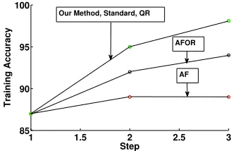
1 1.5 2 2.5 3 85
90 95 100
Step
Training Accuracy
AFOR Our Method, Standard, QR
AF
Figure 10: Training set accuracy of the methods in classifying wafers as in spec or out of spec at the respective steps for logistic regression.
speed after measurements from the finished step become available if we are to take any of the previously mentioned remedial actions.
We consider three critical steps in the manufacturing process with our data spanning over three batches. The first is the wafer polishing step referred to as chemical-mechanical planarization. Here the wafer is smoothed with removal of unnecessary material. During this step, various pressures—viz. condition head pressure, head zone pressures, etc.—and torques are measured indicating the amount of force the wafer is subjected to. The second step we consider is the etching step, where any remaining abnormalities in the photo-resistance on the wafer are removed by plasma ashing. Here the quantity and temperature of the plasma are controlled among other things and corresponding temperatures, pressures and concentrations are measured. The third and final step we consider is the rapid thermal processing step. In this step the electrical properties such as the material dielectric are altered. To alter the electrical properties, the wafer is subjected to sudden temperature ramps at tightly controlled pressures and chemical flows. Hence, here ramp up temperatures, ramp up rates, cool-down rates and various pressures and flows are measured.
By the time the wafer reaches the first step, 2287 measurements are taken. By the second step we have 3317 measurements. Finally we have 4284 measurements by the third step. Each of the three batches have 8926 wafers. In each of the steps, we train over the first batch and test over the second. We then train over the second batch and test over the third. We report the average training time and the average train and test log-likelihoods3 for each step in Tables 3 and 4.
In this experiment, we compare the performance of our algorithms with a) learning from scratch, i.e., standard, b) AFOR, c) AF and d) QR decomposition based updates (Stewart, 2001) or warm starting (QR and WS), for two regression methods, namely, OLS regression and logistic regression (β = D = 0.1) as in the synthetic case. The metric we use to
evaluate the approaches is the time it takes for the local models to find the solution and the corresponding log-likelihood value at the solution. The higher the log-likelihood and the less time it takes to get to it, the better the method. For logistic regression, we discretize
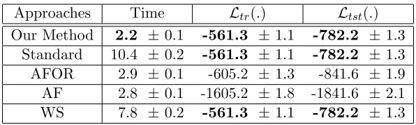
Approaches Time Ltr(.) Ltst(.)
Our Method 2.2 ±0.1 -561.3 ±1.1 -782.2 ±1.3 Standard 10.4 ±0.2 -561.3 ±1.1 -782.2 ±1.3 AFOR 2.9 ±0.1 -605.2 ±1.3 -841.6 ±1.9 AF 2.8 ±0.1 -1605.2 ±1.8 -1841.6 ±2.1 WS 7.8 ±0.2 -561.3 ±1.1 -782.2 ±1.3
Table 5: Average running time (in seconds) of LogitGOMP, the average training log-likelihood valueLtr(.) and the average test log-likelihood valueLtst(.) with a 95% confidence interval.
the target based on specifications to denote either within spec by 1 or out of spec by 0. In all the three batches, roughly 20% of the wafers are out of spec.
5.3.2 Observations
In Tables 3 and 4, we see the results for step 2 and step 3 across the three batches. We do not show step 1 since we have to learn from scratch for all the models. The results show that our methods are optimal and significantly more efficient than the standard method. Our methods are also more efficient than QR and WS. AF and AFOR are efficient since they learn only on the additional features but are sub-optimal. Our methods are almost as efficient as AF and AFOR, which is very encouraging.
In Figures 7, 8, 9 and 10 we observe the test and training set accuracy in classifying wafers as within spec or out of spec based on the predictions obtained from OLS and logistic regression. The OLS predictions of the wafer speed are easily categorized into the two classes by considering the acceptable speed range given in the specification. In all the four figures we see that our method, which is optimal, performs significantly better than AFOR and AF as new features become available, even though it has comparable running time to both of them, as is seen in Tables 3 and 4. The poor performance of AF and AFOR indicates that the features across the various steps are correlated and are required to build an accurate predictive model.
5.4 Group Feature Selection in Finance
regression model, we normalize the revenue, our target, using the sum over the two year period. We divide the data into 8 quarters and perform 8-fold cross-validation as predicting an entire quarter is of more interest than predicting randomly scattered weeks.
Table 5 shows that our method (β = D = 0.1) is almost 5 times faster than the
standard method and about 3.5 times faster than WS. Interestingly, it is also faster than AF and AFOR. The reason for this is that, in the second step, condition two in Algorithm 2 is satisfied and we have the optimal weight matrix and target from the previous update step in LogitGOMP, which is a better starting point than starting from the default during updates.
6. Discussion
It is important to note that the problem addressed in this paper is somewhat complimentary to stagewise learning. Stagewise learning mainly addresses the problem of feature selection, where coefficients are estimated for one feature at a time. Forward selection (Weisberg, 1980) and least angle regression (Efron et al., 2004) are examples of stagewise learning techniques. On the other hand, ours is a meta-learning technique—not limited to any particular regression algorithm—that considers all new features simultaneously with the final goal of learning a predictive model accurately and efficiently.
Our methods are also more general than the incremental feature learning method based on autoencoders to update an existing model(Zhou et al., 2012). This method makes the strong assumption of bounded input and output and the number of features considered at each step is a free parameter. The method is somewhat similar to AFOR as only new features are used to optimize the residual of the model learned over old features. Moreover, our methods are also more general than QR decomposition (Stewart, 2001), which is mainly used for efficient updates in OLS problems.
In the future, it would be interesting to update an existing model simultaneously based on added features and data points rather than doing it sequentially. One may be able to merge the ideas in this paper with the vast online learning literature. However, the main challenge in developing such a method would be guaranteeing accuracy while maintaining efficiency.
Acknowledgments
We would like to thank Katherine Dhurandhar for proofreading the paper.
References
S. Arora, E. Hazan, and S. Kale. The multiplicative weights update method: a meta algorithm and applications. Theory of Computing, 8:121–164, 2005.
A. Blum. On-line algorithms in machine learning. In Workshop on On-Line Algorithms,
Dagstuhl, pages 306–325. Springer, 1996.
L. Bottou and Y. Cun. Large scale online learning. In Neural Information Processing
S. Boyd and L. Vandenberghe. Convex Optimization. Cambridge University Press, New York, NY, USA, 2004.
D. Coppersmith and S. Winograd. Matrix multiplication via arithmetic progressions.
Jour-nal of Symbolic Computation, 9(3):251–280, 1990.
B. Efron, T. Hastie, I. Johnstone, and R. Tibshirani. Least angle regression. Annals of Statistics, 32:407–499, 2004.
G. H. Golub and C. F. Van Loan. Matrix Computations. John Hopkins University Press, 3rd edition, 1996.
T. Hastie, R. Tibshirani, and J. Friedman. The Elements of Statistical Learning: Data
Mining, Inference, and Prediction. Springer, 2nd edition, 2009.
A. E. Hoerl and R. W. Kennard. Ridge regression: Biased estimation for nonorthogonal problems. Technometrics, 12(1):55–67, 1970.
A. Lozano, G. Swirszcz, and N. Abe. Grouped orthogonal matching pursuit for variable selection and prediction. In Neural Information Processing Systems, 2009.
A. Lozano, G. Swirszcz, and N. Abe. Group orthogonal matching pursuit for logistic re-gression. In Artificial Intelligence and Statistics, pages 452–460, 2011.
D. Luenberger. Linear and Nonlinear Programming. Addison-Wesley; 2nd edition, 1984.
P. McCullagh and J. Nelder. Generalized Linear Models, Second Edition. Chapman and Hall, 1990.
D. Pregibon. Logistic regression diagnostics. Annals of Statistics, 9:704–724, 1981.
Y. Saad. Analysis of augmented Krylov subspace methods. SIAM Journal on Matrix
Analysis and Applications, 18(2):435–449, April 1997.
S. Smale and Y. Yao. Online learning algorithms. Found. Comp. Math, 6:145–170, 2005.
G. Stewart. Matrix Algorithms. SIAM, 2001.
R. J. Tibshirani. Regression shrinkage and selection via the LASSO. Journal of the Royal
Statistical Society, Series B, 58:267–288, 1994.
R. J. Tibshirani and J. Taylor. The solution path of the generalized LASSO. The Annals
of Statistics, 39(3):1335–1371, 2011.
P. Wang. Residual plots for detecting nonlinearity in generalized linear models.
Techno-metrics, 29(4):435–438, 1987.
S. Weisberg. Applied Linear Regression. New York: Wiley, 1980.