Policy Gradient in Continuous Time
Rémi Munos [email protected]
Centre de Mathématiques Appliquées Ecole Polytechnique
91128 Palaiseau, France
Editor: Michael Littman
Abstract
Policy search is a method for approximately solving an optimal control problem by performing a parametric optimization search in a given class of parameterized policies. In order to process a local optimization technique, such as a gradient method, we wish to evaluate the sensitivity of the performance measure with respect to the policy parameters, the so-called policy gradient. This paper is concerned with the estimation of the policy gradient for continuous-time, deterministic state dynamics, in a reinforcement learning framework, that is, when the decision maker does not have a model of the state dynamics.
We show that usual likelihood ratio methods used in discrete-time, fail to proceed the gradient because they are subject to variance explosion when the discretization time-step decreases to 0. We describe an alternative approach based on the approximation of the pathwise derivative, which leads to a policy gradient estimate that converges almost surely to the true gradient when the time-step tends to 0. The underlying idea starts with the derivation of an explicit representation of the policy gradient using pathwise derivation. This derivation makes use of the knowledge of the state dynamics. Then, in order to estimate the gradient from the observable data only, we use a stochastic policy to discretize the continuous deterministic system into a stochastic discrete process, which enables to replace the unknown coefficients by quantities that solely depend on known data. We prove the almost sure convergence of this estimate to the true policy gradient when the discretization time-step goes to zero.
The method is illustrated on two target problems, in discrete and continuous control spaces. Keywords: optimal control, reinforcement learning, policy search, sensitivity analysis, para-metric optimization, gradient estimate, likelihood ratio method, pathwise derivation
1. Introduction and Statement of the Problem
We consider an optimal control problem with continuous state(xt∈IRd)t≥0whose state dynamics is defined according to the controlled differential equation:
dxt
dt = f(xt,ut), (1)
where the control(ut)t≥0is a Lebesgue measurable function with values in a control space U . Note that the state-dynamics f may also depend on time, but we omit this dependency in the notation, for simplicity. We intend to maximize a functional J that depends on the trajectory(xt)0≤t≤T over
only:
J(x;(ut)t≥0):=r(xT), (2)
where r : IRd→IR is the reward function. Extension to the case of general functional of the kind
J(x;(ut)t≥0) = Z T
0
r(t,xt)dt+R(xT), (3)
with r and R being current and terminal reward functions, would easily follow, as indicated in Remark 1.
The optimal control problem of finding a control (ut)t≥0 that maximizes the functional is re-placed by a parametric optimization problem for which we search for a good feed-back control law in a given class of parameterized policies{πα:[0,T]×IRd→U}α, whereα∈IRmis the parameter. The control ut ∈U (or action) at time t is ut =πα(t,xt), and we may write the dynamics of the
resulting feed-back system as
dxt
dt = fα(xt), (4)
where fα(xt):=f(x,πα(t,x)). In the paper, we will make the assumption that fαis
C
2, with boundedderivatives. Let us define the performance measure
V(α):=J(x;πα(t,xt)t≥0),
where its dependency with respect to (w.r.t.) the parameterαis emphasized. One may also consider an average performance measure according to some distribution µ for the initial state: V(α):=
E[J(x;πα(t,xt)t≥0)|x∼µ].
In order to find a local maximum of V(α), one may perform a local search, such as a gradient ascent method
α←α+η∇αV(α), (5)
with an adequate stepη(see for example (Polyak, 1987; Kushner and Yin, 1997)). The computation of the gradient∇αV(α)is the object of this paper.
A first method would be to approximate the gradient by a finite-difference quotient for each of the m components of the parameter:
∂αiV(α)≃
V(α+εei)−V(α)
ε ,
for some small value of ε (we use the notation ∂α instead of ∇α to indicate that it is a single-dimensional derivative). This finite-difference method requires the simulation of m+1 trajectories to compute an approximation of the true gradient. When the number of parameters is large, this may be computationally expensive. However, this simple method may be efficient if the number of parameters is relatively small.
Pathwise estimation of the gradient. We now illustrate that if the decision-maker has access to a model of the state dynamics, then a pathwise derivation would directly lead to the policy gradient. Indeed, let us define the gradient of the state with respect to the parameter: zt :=∇αxt (i.e. zt is
defined as a d×m-matrix whose(i,j)-component is the derivative of the ith component of xt w.r.t.
αj). Our smoothness assumption on fαallows to differentiate the state dynamics (4) w.r.t.α, which
provides the dynamics on(zt):
dzt
dt =∇αfα(xt) +∇xfα(xt)zt, (6)
where the coefficients ∇αfα and∇xfα are, respectively, the derivatives of f w.r.t. the parameter
(matrix of size d×m) and the state (matrix of size d×d). The initial condition for z is z0 =0. When the reward function r is smooth (i.e. continuously differentiable), one may apply a pathwise differentiation to derive a gradient formula (see e.g. (Bensoussan, 1988) or (Yang and Kushner, 1991) for an extension to the stochastic case):
∇αV(α) =∇xr(xT)zT. (7)
Remark 1 In the more general setting of a functional (3), the gradient is deduced (by linearity) from the above formula:
∇αV(α) =
Z T
0 ∇x
r(t,xt)ztdt+∇xR(xT)zT.
What is known from the agent? The decision maker (call it the agent) that intends to design a good controller for the dynamical system may or may not know a model of the state dynamics f . In case the dynamics is known, the state gradient zt =∇αxt may be computed from (6) along the
trajectory and the gradient of the performance measure w.r.t. the parameterαis deduced at time T from (7), which allows to perform the gradient ascent step (5).
However, in this paper we consider a Reinforcement Learning (Sutton and Barto, 1998) setting in which the state dynamics is unknown from the agent, but we still assume that the state is fully observable. The agent knows only the response of the system to its control. To be more precise, the available information to the agent at time t is its own control policyπαand the trajectory(xs)0≤s≤t
up to time t. At time T , the agent receives the reward r(xT)and, in this paper, we assume that the
gradient∇r(xT)is available to the agent.
From this point of view, it seems impossible to derive the state gradient zt from (6), since∇αf
and∇xf are unknown. The term∇xf(xt)may be approximated by a least squares method from the
observation of past states(xs)s≤t, as this will be explained later on in subsection 3.2. However the
term∇αf(xt)cannot be calculated analogously.
In this paper, we introduce the idea of using stochastic policies to approximate the state (xt)
and the state gradient(zt)by discrete-time stochastic processes(Xt∆)and(Zt∆)(with∆being some
discretization time-step). We show how Zt∆ can be computed without the knowledge of∇αf , but only from information available to the agent.
We prove the convergence (with probability one) of the gradient estimate ∇xr(XT∆)ZT∆ derived
X
∆tX
∆tX
∆t0 1 2
X
∆Tx
f
αy
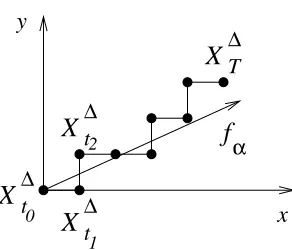
Figure 1: A trajectory (Xt∆n)0≤n≤N and the state dynamics vector fα of the continuous process
(xt)0≤t≤T.
Likelihood ratio method? It is worth mentioning that this strong convergence result contrasts with the usual likelihood ratio method (also called score method) in discrete time (see e.g. (Reiman and Weiss, 1986; Glynn, 1987) or more recently in the reinforcement learning literature (Williams, 1992; Sutton et al., 2000; Baxter and Bartlett, 2001; Marbach and Tsitsiklis, 2003)) for which the policy gradient estimate is subject to variance explosion when the discretization time-step∆tends to 0. The intuitive reason for that problem lies in the fact that the number of decisions before getting the reward grows to infinity when∆→0 (the variance of likelihood ratio estimates being usually linear with the number of decisions).
Let us illustrate this problem on a simple 2 dimensional process. Consider the deterministic continuous process(xt)0≤t≤1defined by the state dynamics:
dxt
dt = fα:=
α
1−α
, (8)
(0<α<1) with initial condition x0 = (0 0)′ (where ′ denotes the transpose operator). The per-formance measure V(α)is the reward at the terminal state at time T =1, with the reward function being the first coordinate of the state r((x y)′):=x. Thus V(α) =r(x
T=1) =αand its derivative is ∇αV(α) =1.
Let (Xt∆n)0≤n≤N ∈IR2 be a discrete time stochastic process (the discrete times being {tn =
n∆}n=0...N with the discretization time-step∆=1/N) that starts from initial state X0∆=x0= (0 0)′ and makes N random moves of length ∆towards the right (action u1) or the top (action u2) (see Figure 1) according to the stochastic policy (i.e., the probability of choosing the actions in each state x)πα(u1|x) =α,πα(u2|x) =1−α.
The process is thus defined according to the dynamics:
Xt∆n+1=Xt∆n+
Un
1−Un
∆, (9)
where(Un)0≤n<Nare N independent Bernoulli random variables that equal 1 with probabilityαand
dynamics vector of the latter:
EhXtn+1−Xtn
∆ |Xtn =x
i
=πα(u1,x)
1 0
+πα(u2,x)
0 1
=
α
1−α
.
Thus, when the discretization time-step∆tends to 0, the process(Xt∆)converges almost surely to(xt)(this statement will be proved in Section 2).
Now, write V∆(α)the performance measure of the discrete process, taken as the expected reward at the terminal state: V∆(α):=E[r(X1∆)] = N1∑N−n=01Un. The likelihood ratio estimate g(∆) of the
gradient∇αV∆(α) =E[g(∆)]is
g(∆) = r(X1∆)
N−1
∑
n=0
∇απα(utn|Xt∆n)
πα(utn|Xt∆n)
= 1 N
N−1
∑
n=0 Un
N−1
∑
n=0 Un
α − 1−Un
1−α
. (10)
The expectation and variance of this estimate are given now (a proof is provided in Appendix A).
Proposition 2 The expectation and variance of the estimate (10) are
Eg(∆) = 1,
Varg(∆) = 1−5(1−α) + (2−3α)αN+α 2N2
α(1−α)N . (11)
Thus g(∆) is an unbiased estimated of the true gradient∇αV(α) =1. However we notice that the dominant term (when N is large) of the variance is 1−ααN, with N being the number of decisions before getting the reward, which grows to infinity when the discretization time-step∆=1/N tends to 0. Therefore it is impossible to use this likelihood ratio estimate whenever the time discretization is too fine. In contrast, the gradient estimate introduced in this paper has a variance that decreases to 0 when∆tends to 0 (this will be illustrated on this same example in subsection 3.4).
Outline of the paper. The paper is organized as follows: in Section 2, we state a general approx-imation result of a continuous deterministic process by a consistent stochastic discrete process and apply it to prove the convergence of the discretized state and state gradient processes when using a stochastic policy. In Section 3, we establish the convergence of the policy gradient estimate and describe a reinforcement learning algorithm that replaces the unknown coefficients about the state dynamics by information available to the agent. In the last Section, we illustrate the method on two (6 dimensional) target problems in both a discrete and a continuous control space cases. All proofs are in the Appendices.
2. Discretized Stochastic Processes
2.1 A General Convergence Result
Let(xt)0≤t≤T be a deterministic continuous process defined by some dynamics
dxt
dt = f(xt)
with some initial condition x0. We assume that f is of class
C
2 with bounded derivatives. The following result state the almost sure convergence of a consistent discrete stochastic process.Theorem 3 Let ∆=T/N be a discretization time-step (with N being the number of steps) and write {tn=n∆}0≤n≤N the discrete times. Let (Utn)0≤n<N be a sequence of independent random
variables with values in a set U . We define a discrete stochastic process(Xt∆n)0≤n≤N, starting at
X0∆=x0, according to some discrete state dynamics f∆ : IRd×U→IRd, assumed to be bounded: for t∈ {tn}0≤n<N ,
Xt∆+∆=Xt∆+f∆(Xt∆,Ut). (12)
If f∆satisfies the consistency property:
E[f∆(x,Ut)] = f(x)∆+o(∆), (13)
and the following bounding condition:
f∆=O(∆), (14)
(where the notation O(·)is to be understood in the sense uniformly w.r.t. the variable of f∆) then, the random variable XT∆converges almost surely to (the deterministic) xT when∆→0. We write
lim ∆→0X
∆
T =xT,with probability 1.
Appendix B gives a proof of this result. Note that a weaker convergence result (i.e. convergence in probability) may be obtained from general results in approximation of diffusion processes by Markov chains (Kloeden and Platen, 1995). Here, almost sure convergence is obtained using the concentration of measure phenomenon (Talagrand, 1996; Ledoux, 2001), detailed in Appendix B.
Remark 4 If we assume a slightly better consistency error of O(∆2)instead of o(∆)in (13), then we may prove (straightforwardly from the Appendix) thatE[XT∆] =xT+O(∆)andE[||XT∆−xT||2] =
O(∆).
2.2 Discretization of the State
Let us go back to our initial control problem (1). We consider the case of a finite control space U (extension to a continuous control space is straightforward and is detailed in subsection 3.5). Letπα be a stochastic policy , i.e. πα(u|t,x)denotes the probability of choosing action u∈U at time t in state x. We write u∼πα(·|t,x)a random choice of an action u according to such a policy.
Now, we define the stochastic discrete state process(X∆t
n)0≤n≤N(where we use the same
no-tations for the time-steps(tn)as in the previous subsection), starting at a state X0∆=x, as follows: At time t ∈ {(tn)0≤n<N}, we select an action ut ∼πα(·|t,Xt∆). Then, Xt∆+∆ is the state at time
t+∆resulting from keeping the action ut constant for a period of time∆. We write:
ut ∼ πα(·|t,Xt∆)
Xt∆+∆ := Xt∆+f∆(Xt∆,ut)
where f∆(x,u) represents the jump in the state resulting from the state dynamics (1) with initial condition x0=x, using a constant control u for a period of time∆.
The next proposition states the convergence of the discrete stochastic process(Xt∆)to the con-tinuous deterministic one(xt).
Proposition 5 Convergence of the discrete state process(X∆t). When the discretization time-step ∆→0, the random variable XT∆ converges almost surely to the state xT defined according to the
state dynamics (4) with
fα(x):=
∑
u∈U
πα(u|t,x)f(x,u).
and initial condition x0=x.
Proof This is an immediate consequence of Theorem 3 with the discrete state dynamics f∆(x,u). From Taylor’s formula,
f∆(x,ut) = f(x,ut)∆+O(∆2),
to derive the property on the average jumps:
E[f∆(x,ut)] =
∑
u∈U
πα(u|t,x)f(x,u)∆+O(∆2) = fα(x)∆+O(∆2),
and the consistency conditions (13) holds, as well as the bound on the jumps (14).
2.3 Discretization of the State Gradient
Now, we build an approximation of the state gradient zt =∇αxt. We define the stochastic discrete
state gradient process(Z∆tn)0≤n≤N, starting with Z0∆=0, as follows:
At time t∈ {(tn)0≤n<N}, let(ut)and(Xt∆)be defined according to (15). Then define
Zt∆+∆:=Zt∆+f(Xt∆,ut)
lα(t,Xt∆,ut)′+lx(t,Xt∆,ut)′Zt∆ ∆
+∇xf(Xt∆,ut)Zt∆∆, (16)
where
lα(t,x,u):=∇απα(u|t,x)
πα(u|t,x) and lx(t,x,u):=
∇xπα(u|t,x)
πα(u|t,x)
are the likelihood ratios ofπαw.r.t.αand x (defined as vectors of size m and d respectively).
Proposition 6 Convergence of the discrete state gradient process(Z∆T):
The random variable Z∆T converges almost surely to zT when∆→0.
Proof The discrete state dynamics (12) for (Zt∆) is defined by the right hand side of (16). Now, from the property
E[Zt∆+∆−Zt∆|Xt∆=x,Zt∆=z] =
∑
u∈U
πα(u|t,x)nf(x,u)[lα(t,x,u)′+lx(t,x,u)′z]
+∇xf(x,u)z o
∆
= ∇αfα(x) +∇xfα(x)z
we deduce that the coupled process(Xt∆,Zt∆)is consistent with(xt,zt)in the sense of (13):
E
Xt∆+∆ Zt∆+∆
−
Xt∆ Zt∆
Xt∆ Zt∆
=
x z
=
fα(x) ∇αfα(x) +∇xfα(x)z
∆+o(∆) (17)
and Xt∆+∆−Xt∆=O(∆)and Zt∆+∆−Zt∆=O(∆). Thus, as a consequence of Theorem 3, the random variable ZT∆converges almost surely to zT when∆→0.
3. Model-Free Reinforcement Learning Algorithm
We show how to use the approximation results of the previous section to design a model-free rein-forcement learning algorithm for estimating the policy gradient∇αV(α)using one trajectory only. First, we state the convergence of the policy gradient estimate computed from the discretized pro-cess, then show how to approximate the unknown coefficient ∇xf using least-squares regression
from the observed trajectory, and finally describe the reinforcement learning algorithm.
3.1 Convergence of the Policy Gradient Estimate
One may use formula (7) to define a gradient estimate of the performance measure w.r.t. the param-eterαbased on the discrete process(Xt∆,Zt∆):
g(∆):=∇xr(XT∆)ZT∆. (18)
This estimate converges almost surely to the true gradient, as stated now.
Proposition 7 Assume that r is continuously differentiable. Then
lim
∆→0g(∆) =∇αV(α)with probability 1.
Proof This is a direct consequence of the almost sure convergence of(XT∆,Z∆T)to(xT,zT)and the
continuity of∇xr.
Now, let us illustrate how Zt∆ may be approximated with information available to the agent. The definition (16) of Zt∆ requires the term ∇xf(Xt∆,u). We now explain how to built a consistent
approximation∇dxf(Xt∆,u)of this term from the past of the trajectory(Xs∆)0≤s≤t.
3.2 Least-Squares Approximation of∇xf(Xt∆,u)
For clarity, in this subsection, we omit reference to∆, for example writing Xsinstead of Xs∆. Write
∆Xt =Xt+∆−Xt the jump of the state. Let c>0 be a constant (independent of∆). Define S(t):=
{s∈[t−c∆,t]|us =ut} the set of past discrete times t−c∆≤s≤t when action ut have been
chosen. Note that the cardinality of S(t)is independent from ∆, and solely depends on c and the actual sequence of controls chosen according to the stochastic policyπα.
From Taylor’s formula, for all discrete time s,
∆Xs=Xs+∆−Xs=f(Xs,ut)∆+∇xf(Xs,ut)f(Xs,ut)
∆2 2 +O(∆
Now, for s∈S(t)we have Xt−Xs=O(∆), thus
f(Xs,ut) = f(Xt,ut) +∇xf(Xt,ut)(Xs−Xt) +O(∆2),
from which we deduce (using the fact that∇xf(Xs,ut) =∇xf(Xt,ut) +O(∆)) that
∆Xs = ∆Xt+ ∇
xf(Xs,ut)f(Xs,ut)−∇xf(Xt,ut)f(Xt,ut) ∆2
2 +∇xf(Xt,ut)(Xs−Xt)∆+O(∆3)
= ∆Xt+∇xf(Xt,ut)[Xs−Xt+
1
2(∆Xs−∆Xt)]∆+O(∆
3) (20)
= b+A(Xs+
1
2∆Xs)∆+O(∆ 3)
with b :=∆Xt−∇xf(Xt,ut)(Xt+12∆Xt)∆and A :=∇xf(Xt,ut). Based on the observation of several
jumps {∆Xs}s∈S(t), one may derive an approximation of ∇xf(Xt,ut) by solving the least-squares
problem:
min
A,b
1 nts∈S
∑
(t)
∆Xs−b−A Xs+
1 2∆Xs
∆
2
, (21)
where nt is the cardinality of S(t). Write Xs+:=Xs+12∆Xs= 12(Xs+Xs+∆) and use the simplified
notations: X , X X′,∆X , and∆X X′, to denote the average values, when s∈S(t), of Xs+, Xs+(Xs+)′, ∆Xs, and∆Xs(Xs+)′, respectively. For example,
X := 1
nts∈S
∑
(t)Xs+.
The optimality condition for (21) holds when the matrix Qt:=X X′−X X ′
is invertible, and in that case, the least squares solution provides the approximation∇dxf(Xt,ut)of∇xf(Xt,ut):
d
∇xf(Xt,ut) =
1
∆ ∆X X′−∆X X
′
X X′−X X′−1. (22)
This optimality condition does not hold when the set of points(Xs+)s∈S(t)lies in a vector space
of dimension <d (then, Qt is degenerate). In order to circumvent this problem, we assume that
the eigenvalues of the matrix Qt are bounded away from 0, in the sense given in the following
proposition (whose proof in provided in Appendix C).
Proposition 8 The matrix Qt=X X′−X X′is symmetric non-negative. Letν(∆)≥0 be the smallest
eigenvalue of Qt, for all 0≤t≤T . Then, ifν(∆)>0 andν(∆)satisfies
1
ν(∆)=o(∆
−4), (23)
then, for all 0≤t≤T , the least squares estimate∇dxf(Xt,ut)defined by (22) is consistent with the
gradient∇xf(Xt,ut), that is:
lim ∆→0
d
The condition (23) is not easy to check since it depends on the state dynamics and the policy. Note however that, when we use a strict stochastic policy (i.e.,πα>0), a sufficient condition for the set of points(Xs+)s∈S(t)to span a vector space of dimension d is that the system be (at least locally)
controllable. In the case of linear systems dx/dt=Ax+Bu, where u∈U=IRq, and A and B being d×d and d×q-matrices respectively, a necessary and sufficient condition for controllability is that the d×(qd)controllability matrix[B : AB : A2B :· · ·: Ad−1B]has rank d (this is the so-called Kalman rank condition (Kalman et al., 1969)). In more general settings, for example when f is a linear combination of vector fields hi(x)weighted by the control components, i.e. f(x,u) =∑qi=1hi(x)ui,a
sufficient condition for controllability is that the dimension of the Lie algebra generated by the fields {hi} is d (see e.g. (LaValle, 2006)). Intuitively, this dimension represents the number of possible
independent directions of movement when following any sequence of controls. In our numerical experiments, we observed the convergence of the∇xf estimate.
Remark 9 A simple on-line way for approximating∇xf is to consider a weighted least-squares
problem using an exponential weight (with some coefficientλ∈(0,1)) instead of the rectangular window s∈[t−c∆,t]. The piece of information related to a time s<t is weighted byλp, where p is the number of times the control u has been chosen between s and t. It is easy to adapt the proof of Proposition 8 to derive that a such weighted least squares estimate for∇xf is consistent, for any
λ∈(0,1), under the same condition (23).
An on-line update rule would consider tables for the average values Y(u)(where Y means X , X X′, ∆X , or ∆X X′) for all u∈U . The values are initialized (at the first time t each action u is encountered) by Yt, where Yt means Xt+, Xt+(Xt+)′, ∆Xt, and∆Xt(Xt+)′, respectively. Then, the
values are updated at time t, according to
Y(u)←λY(u) + (1−λ)Yt for u=ut,
Y(u)stays unchanged for u6=ut.
The quantities X , X X′,∆X , and∆X X′ are easily updated and the estimate∇d
xf may
advanta-geously be computed from (22) by using an iterative matrix inversion, such as with the Sherman-Morrison formula (see for example (Golub and Loan, 1996)).
Note that for the first discrete times t, the matrix X X′−X X′ may not be invertible, simply because there is not enough points(Xs)s<t to form a subspace of dimension d. We may simply set
d
∇xf to 0, which has no impact on the general convergence result.
3.3 The Reinforcement Learning Algorithm
Here, we derive a convergent policy gradient estimate in which all information required to build the state gradient Zt∆is the past trajectory(Xs∆)0≤s≤t.
Choose a time step∆. For a given stochastic policyπα, the algorithm proceeds as follows:
1. At time t=0, initialise X0∆=x and Z0∆=0.
2. For each discrete time t ∈ {(tn)0≤n<N}, choose an action ut ∼πα(t,Xt∆) according to the
3. Update the average values X , X X′,∆X , or∆X X′, for all u∈U , as described in subsection 3.2, for example by using an exponential trace with parameterλ∈(0,1)as mentioned in Remark 9.
4. Compute the state dynamics gradient approximation∇dxf(Xt∆,ut)according to
d
∇xf(Xt∆,ut) =
1
∆ ∆X X′−∆X X
′
X X′−X X′−1.
5. Update Zt∆according to
Zt∆+∆ = Zt∆+∆Xt∆h∇απα(ut|t,X ∆
t ) ′
πα(ut|t,Xt∆)
+
∇xπα(ut|t,Xt∆) ′
πα(ut|t,Xt∆)
Zt∆i
+∇dxf(t,Xt∆,ut)Zt∆∆. (24)
6. Repeat steps 2-5 until t=T . Then return the policy gradient estimate∇xr(XT∆)ZT∆.
This algorithm returns a consistent approximation of the policy gradient∇αV(α), as stated now.
Proposition 10 Assume that the property (23) of Proposition 8 holds, and that the reward function is continuously differentiable. Then the estimate ∇xr(XT∆)Z∆T returned by the RL algorithm is a
consistent approximation of the policy gradient∇αV(α), in the sense that ∇xr(XT∆)Z∆T converges
almost surely to∇αV(α)when∆→0.
Proof From Proposition 8,∇dxf is a consistent approximation of∇xf , thus the process(Zt∆)built
from (24) also satisfies the consistency condition (17), and the proof follows like in Proposition 7.
3.4 Illustration on a Simple Example
Let us illustrate this algorithm on the simple example described in the introduction (for which we observed the infinite variance of the likelihood ratio estimate in the continuous time limit).
The continuous process is defined by (8) and the discrete time stochastic process by (9). With the notations used in the introduction, the state gradient dynamics (24) is:
Zt∆n+1=Zt∆n+ (Xt∆n+1−Xt∆n)∇απα(utn|t,Xt∆n)
πα(utn|t,Xt∆n)
=Zt∆+
Un/α
(1−Un)/(α−1)
∆.
Thus the gradient estimate (18) is
g(∆) =∇r(XT∆=1)Z∆T=1,1= 1 αN
N−1
∑
n=0 Un
.
Since E[g(∆)] =1, this is an unbiased estimate of the true gradient ∇αV(α) =∇αr(x1) =1. Moreover, its variance Var[g(∆)] = 1
α2NVar[Un] =1α−Nαdecreases to 0 when N goes to infinity, which
u
t
t
ε
∆
α
h
αh (t, X )
t
∆
t
t, X
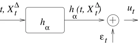
Figure 2: A stochastic policy ut =hα(t,Xt∆) +εt withεt∼
N
(0,v(∆)).3.5 The Continuous Control Space Case
So far, we have used notations for a finite control space U . However, the same results hold in the case of a continuous control space U∈IRq. Let us illustrate a simple way for defining a stochastic policy based on a parameterized deterministic policy. Let hα:[0,T]×IRd →U =IRqbe a deterministic policy parameterized by α (which may be implemented by a neural network, or with any other function approximator). We search for a value of the parameterαthat maximizes the performance of the corresponding policy.
We build a stochastic policy by perturbing hα with a centered Gaussian noise of covariance matrix v(∆) (i.e. which depends on the discretization time-step∆). Thus ut =hα(t,Xt∆) +εt with
εt∼
N
(0,v(∆)). See Figure 2. We assume that lim∆→0v(∆) =0.This stochastic policy admits a probability density representationπα(u|t,x):
πα(u|t,x) =p 1
(2π)p|v(∆)|exp h
−1
2(u−hα(t,x))
′v(∆)−1(u−h α(t,x))
i .
The stochastic process(Xt∆)built according to (15) from this stochastic policyπαis consistent with the continuous process(xt)defined by the parameterized deterministic policy hα:
dxt
dt =f(x,hα(t,x)).
Indeed, from the continuity of f , and the assumption that v(∆)∆−→→00, the average state dynamics vector using the stochastic policyπαtends to the state dynamics vector using the deterministic policy hα:
lim ∆→0
Z
IRq f(x,u)πα(u|t,x)du= f(x,hα(t,x)),
and the consistency property (13) as well as the bound (14) hold (for the same reasons as those invoked in subsection 2.2). Thus, the reinforcement learning algorithm of subsection 3.3 applies directly.
Note that from the specific form of the policyπα(u|t,x), the likelihood ratios are easily com-puted: for each parameterαi, 1≤i≤m, ∂αiπα
(u|t,x)
πα(u|t,x) =∂αihα(t,x)v(∆)
−1(u−h
α(t,x)), and for each
coordinate xi, 1≤i≤d, ∂xiπα
(u|t,x)
πα(u|t,x) =∂xihα(t,x)v(∆)
−1(u−h
4. Numerical Experiments
We provide two experiments, a target problem and an inverted pendulum, that illustrate the rein-forcement learning algorithm described in subsection 3.3 in the case of a finite and a continuous control space, respectively.
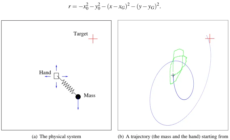
4.1 A Target Problem
This is a 6 dimensional system(x0,y0,x,y,vx,vy)that represents a hand ((x0,y0)position) holding a spring to which is attached a mass (defined by its position(x,y)and velocity(vx,vy)) subject to
gravitation. The control is the movement of the hand, in any 4 possible directions (up, down, left, right). The goal is to reach a target(xG,yG)with the mass at a specific time T (see Figure 3a), while
keeping the hand close to the origin. For that purpose, the terminal reward function is defined by
r=−x20−y20−(x−xG)2−(y−yG)2.
Hand
Mass Target
(a) The physical system (b) A trajectory (the mass and the hand) starting from the origin
Figure 3: (a) the physical system. (b) A trajectory obtained after 1000 gradient steps. For that specific trajectory, the performance (terminal reward) was−0.087.
The state dynamics is:
˙
x0=ux, x˙=vx, v˙x=−mk(x−x0), ˙
y0=uy, y˙=vy, v˙y=−mk(y−y0)−g,
with k being the spring constant, m the mass, g the gravitational constant, and (ux,uy) =u∈
U :={(1,0),(0,1),(−1,0),(0,−1)}the control. We consider a Boltzmann-like stochastic policy
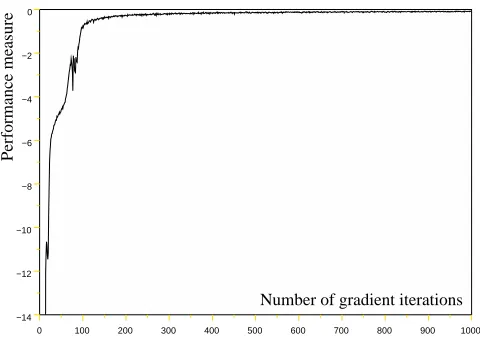
0 100 200 300 400 500 600 700 800 900 1000 −14
−12 −10 −8 −6 −4 −2 0
Performance measure
Number of gradient iterations
Figure 4: Performance of successive parameterized controllers.
with a linear parameterization of the Qαvalues: Qα(t,x,u) =αu
0+αu1t+αu2x0+αu3y0+αu4x+αu5y+ αu
6vx+αu7vy, for each 4 possible actions u∈U . Thus the parameterα∈IR32. We initializedαwith
uniform random values in the range[−0.01,0.01]. In our experiments we chose k=1, m=1, g=1, xG=yG=2,λ=0.9,∆=0.01, T =10.
At each iteration, we run one trajectory (Xt)0≤t≤T using the stochastic policy, and calculate
the policy gradient estimate according to the RL algorithm described in subsection 3.3. We then perform a gradient ascent step (5) (with a fixed stepη=0.01). Figure 4 shows the performance of the parameterized controller as a function of the number of gradient iterations.
For that problem, we chose initial states uniformly distributed over the domain [−0.1,0.1]6. We found that the randomness introduced in the choice of the initial state helped in not getting stuck in local minima. Here, convergence of the gradient method occurs to a controller close to optimality (for which r=0). We illustrate in Figure 3b the trajectory (where only the hand and the mass positions are shown) obtained after 1000 gradient steps, starting from the initial state (x0,y0,x,y,vx,vy)t=0=0.
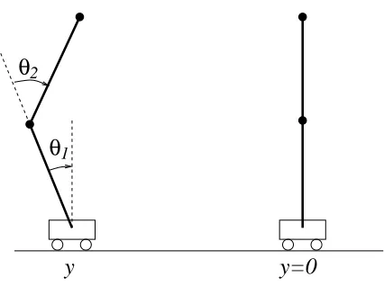
4.2 Double Inverted Pendulum
We illustrate the approach described in subsection 3.5 on this continuous control space problem. This is an double inverted pendulum defined in the 6-dimensions: the position of the cart, its ve-locity, the two angles, and their angular velocity x= (y,v,θ1,ω1,θ2,ω2)′∈IR6(see Figure 5). The control u∈U=IR (continuous variable) is the force applied to the cart. The state dynamics are de-scribed in (Bogdanov, 2004). The goal is to reach the unstable equilibrium(y,v,θ1,ω1,θ2,ω2) =0 at time T =5. We consider the quadratic reward function r(x) =−(y2+v2+θ2
determin-θ
θ
1 2
y=0
y
Figure 5: The double inverted pendulum. Current position and target position.
istic policy hα(t,x) =α1+α2y+α3v+α4θ1+α5ω1+α6θ2+α7ω2, i.e. the control at time t is ut∼hα(t,xt) +
N
(0,v(∆)).We wish to find a local maximum of the performance measure V(α) =r(xT)in the space of the
policy parametersα∈IR7. We initializedαwith uniform random values in the range[−0.01,0.01], and perform a stochastic gradient algorithm (5) where the gradient∇αV(α)is computed according to the reinforcement learning algorithm defined in subsection 3.3.
A gradient step update (5) is performed (with η=1) at the end of each sample trajectory starting from an initial state, chosen uniformly randomly in the domain defined by y∈[−1,1], θ1∈[−0.3,0.3], θ2∈[−0.3,0.3], and v=0, ω1=0, ω2=0. We use a discretization time-step ∆=10−3which is low enough to provide a very good approximation of the true gradient, that is the gradient that would be obtained from the continuous (but unknown from the agent) state dynamics by using the deterministic policy hα(t,x).
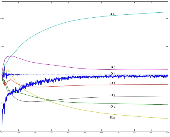
Figure 6 shows (in bold) the performance measure (terminal reward) at the end of each tra-jectory as a function of the number of gradient iterations. The other curves give the values of the (α1, . . . ,α7)during simulations.
After 1000 gradient iterations, the obtained policy is hα(t,x) =−0.0023−5.31y−1.74v+ 11.16θ1+0.92ω1−7.77θ2−3.94ω2, and the resulting average performance is−0.097 for trajecto-ries starting randomly from the same domain as during learning. In this problem, a linear controller is sufficient to derive a controller close to optimality. However, we should mention that for initial states in another domain (say, if the angles were not close to 0, and loops would be required to reach the target position), the problem would not possibly be solved with such a simple class of policies.
5. Conclusion
0 100 200 300 400 500 600 700 800 900 1000 −10 −5 0 5 10 4 α α α α α α α 5 1 3 7 2 6
Figure 6: The bold curve shows the performance measure V(α), and the other curves the values of (α1, . . . ,α7), as a function of the number of gradient iterations.
In future work, it would be interesting to extend this method to the case of stochastic dynamics, and to non-smooth reward functions (or in case the reward gradient is unknown from the agent), by using integration-by-part formula for the gradient estimate, such as the likelihood ratio method of (Yang and Kushner, 1991) or the martingale approach of (Gobet and Munos, 2005).
Appendix A. Proof of Proposition 2
The likelihood ratio estimate (10) may be rewritten
g(∆) = 1
α(1−α)N
N−1
∑
n=0 Un
N−1
∑
n=0
Un−α
= 1
α(1−α)N
h N−1
∑
n=0 Vn
2 +αN
N−1
∑
n=0 Vn
i ,
with Vn:=Un−α. From the fact thatE[Vn2] =α(1−α), the expectation of the estimate is
E[g(∆)] = 1
α(1−α)NE
N−1
∑
n=0 Vn
2 =1.
Now its variance Var[g(∆)]is
1
[α(1−α)N]2Cov
h N−1
∑
n=0 Vn
N−1
∑
p=0 Vp
+αN
N−1
∑
n=0 Vn,
N−1
∑
n′=0
Vn′ N−1
∑
p′=0
Vp′+αN N−1
∑
n=0 Vn′
i
Notice that from the independence of the Bernoulli random variables(Un), all terms Cov(Vn,Vn′) =
0 for n6=n′, and Cov(Vn,Vn) =E[(Un−α)2] =α(1−α).
The terms Cov(Vn,Vn′Vp′) =EVn(Vn′Vp′−E[Vn′Vp′])=E[VnVn′Vp′](because Vn is centered)
equal 0 whenever n6=n′or n6=p′. And Cov(Vn,Vn2) =E[Vn3] =α(1−α)(1−2α).
Now, Cov(VnVp,Vn′Vp′) =0 when n6=n′, n6=p′, p6=n′, and p6=p′(because the variables VnVp
and Vn′Vp′are independent). The terms Cov(VnVp,VnVp′) =E(VnVp−E[VnVp])(VnVp′−E[VnVp′])= E[VnVpVnVp′] =0 for n6=p, n6=p′, and p=6 p′(independence of Vpand Vn2Vp′). Now, Cov(VnVp,VnVp) = E[(VnVp)2] =α2(1−α)2 when n6=p. Finally, Cov(Vn2,Vn2) =E[Vn4]− E[Vn2]
2
=α(1−α)(1− 3α+3α2)−α2(1−α)2=α(1−α)(1−4α+4α2).
Thus, the covariance term in (25) is
Nα(1−α)(1−4α+4α2) +N(N−1)α2(1−α)2+αN2α(1−α)(1−2α) +α2N3α(1−α) and the variance of the likelihood ratio estimate is
Var[g(∆)] =1−5(1−α) + (2−3α)αN+α 2N2
α(1−α)N .
Appendix B. Proof of Theorem 3
For convenience, we write xnfor xtn, Xnfor Xt∆n, unfor utn, and Unfor Utn, 0≤n≤N. Let us define the
average approximation errors m∆n =E[||Xn−xn||]and the squared errors v∆n =E[||Xn−xn||2]. Here,
we prove the convergence at the terminal time T , i.e. that XT →xT almost surely when∆→0.
B.1 Convergence of the Squared ErrorE[||XT∆−xT||2]:
We use the decomposition:
v∆n+1 = E[||Xn+1−Xn||2] +E[||Xn−xn||2] +E[||xn−xn+1||2]
+2E[(Xn−xn)′(Xn+1−Xn+xn−xn+1)] (26)
+2E[(Xn+1−Xn)′(xn−xn+1)].
From the bounded jumps property (14),E[||Xn+1−Xn||2] =O(∆2). From Taylor’s formula,
xn+1−xn= f(xn)∆+O(∆2), (27)
thus E[||xn−xn+1||2] =O(∆2) (since f is Lipschitz, and xt and f(xt) are uniformly bounded on
[0,T]) and from Cauchy-Schwarz inequality,|E[(Xn+1−Xn)′(xn−xn+1)]|=O(∆2). From (13) and (27),
E[Xn+1−Xn+xn−xn+1|Xn] = [f(Xn)−f(xn)]∆+o(∆). (28)
Now, from (14) we deduced that||Xn−x0||=O(1)thus Xnis bounded (for all n and N), as well as
xn. Let B a constant such that||Xn|| ≤B and||xn|| ≤B for all n≤N, N≥0. Since f is
C
2, fromTaylor’s formula, there exists a constant k, such that, for all n≤N,
We deduce that
|E[(Xn−xn)′(Xn+1−Xn+xn−xn+1)]|=
E(Xn−xn)′(f(Xn)−f(xn))∆+o(∆)
≤E(Xn−xn)′∇xf(xn)(Xn−xn)∆+2kBvn∆+o(∆)
≤Mv∆n∆+o(∆)
with M=sup||x||≤B||∇xf(x)||+2kB. Thus, (26) leads to the recurrent bound
v∆n+1≤(1+M∆)v∆n+o(∆).
This actually means that there exists a function e(∆)→0 when ∆→0, such that v∆n+1 ≤(1+ M∆)v∆n+e(∆)∆. Thus,
v∆N≤(1+M∆)
N−1
(1+M∆)−1 e(∆)∆≤(e
NM∆−1)1
Me(∆)
thus vN∆ =o(1), that isE[||XT∆−xT||2]∆ →0 −→0.
B.2 Convergence of the MeanE[||XT∆−xT||]:
From (28), we have
E[Xn+1−xn+1|Xn] =Xn−xn+ [f(Xn)−f(xn)]∆+o(∆).
Thus from (29),
m∆n+1=E[||Xn+1−xn+1||] ≤ (1+||∇xf(xn)||∆)E[||Xn−xn||] +kv∆n∆+o(∆)
≤ (1+M′∆)m∆n+o(∆),
since v∆n=o(1)(with M′=sup||x||≤B||∇xf(x)||). Using the same deduction as above, we obtain that
m∆N=o(1), that isE[||XT∆−xT||]∆−→→00.
B.3 Almost Sure Convergence
Here, we use the concentration-of-measure phenomenon (Talagrand, 1996; Ledoux, 2001), which states that under mild conditions, a function (say Lipschitz or with bounded differences) of many independent random variables concentrates around its mean, in the sense that the tail probability decreases exponentially fast.
From the definition of the discrete state process (12), one may write the state XNas a function h
of the independent random variables(Un)0≤n<N, i.e.
XN−x0=h(U0, . . . ,UN−1):= N−1
∑
n=0
(Xn+1−Xn). (30)
Observe that h−E[h] =∑N−1
n=0 dnwith dn=Xn+1−Xn−E[Xn+1−Xn]being a martingale
differ-ence sequdiffer-ence (that isE[dn|U0, . . . ,Un−1] =0). Now, from (Ledoux, 2001, lemma 4.1), one has:
for any D2≥∑N−1
n=0||dn||∞2. Thus, from (14), and since f∆(Xn) is bounded (for all n<N and all
N>0), there exists a constant C that does not depend on N such that dn≤C/N. Thus we may take
D2=C2/N.
Now, from the previous paragraph, ||E[XN]−xN|| ≤e(N), with e(N)→0 when N→∞. This
means that||h−E[h]||+e(N)≥ ||XN−xN||,thus
P(||h−E[h]|| ≥ε+e(N))≥P(||XN−xN|| ≥ε),
and we deduce from (31) that
P(||XN−xN|| ≥ε)≤2e−N(ε+e(N))
2/(2C2)
.
Thus, for all ε>0, the series∑N≥0P(||XN−xN|| ≥ε) converges. Now, from Borel-Cantelli
lemma, we deduce that for allε>0, there exists Nεsuch that for all N≥Nε,||XN−xN||<ε, which
proves the almost sure convergence of XN to xNas N→∞(i.e. XT ∆→
0
−→xT almost surely).
Appendix C. Proof of Proposition 8
First, note that Qt=X X′−X X′is a symmetric, non-negative matrix, since it may be rewritten as
1 nt s∈S
∑
(t)(Xs+−X)(Xs+−X)′.
In solving the least squares problem (21), we deduce b=∆X+AX∆, thus
min
A,b
1 nts∈S
∑
(t)
∆Xs−b−A(Xs+
1 2∆Xs)∆
2 =min A 1 nts∈S
∑
(t)
∆Xs−∆X−A(Xs+−X)∆ 2
≤ 1 nts∈S
∑
(t)
∆Xs−∆X−∇xf(X,ut)(Xs+−X)∆ 2
. (32)
Now, since Xs=X+O(∆)one may obtain like in (19) and (20) (by replacing Xt by X ) that:
∆Xs−∆X−∇xf(X,ut)(Xs+−X)∆=O(∆3). (33)
We deduce from (32) and (33) that
1 nts∈S
∑
(t)
d∇xf(Xt,ut)−∇xf(X,ut)
(Xs+−X)∆2=O(∆6).
By developing each component,
d
∑
i=1
d∇xf(Xt,ut)−∇xf(X,ut)
row iQtd∇xf(Xt,ut)−∇xf(X,ut) ′
row i=O(∆
4). Now, from the definition ofν(∆), for all vector u∈IRd, u′Qtu≥ν(∆)||u||2, thus
ν(∆)||∇dxf(Xt,ut)−∇xf(X,ut)||2=O(∆4).
Condition (23) yields∇dxf(Xt,ut) =∇xf(X,ut) +o(1), and since∇xf(Xt,ut) =∇xf(X,ut) +O(∆),
we deduce
lim ∆→0
d
References
J. Baxter and P. L. Bartlett. Infinite-horizon gradient-based policy search. Journal of Artificial Intelligence Research, 15:319–350, 2001.
A. Bensoussan. Perturbation methods in optimal control. Wiley/Gauthier-Villars Series in Modern Applied Mathematics. John Wiley & Sons Ltd., Chichester, 1988. Translated from the French by C. Tomson.
A. Bogdanov. Optimal control of a double inverted pendulum on a cart. Technical report CSE-04-006, CSEE, OGI School of Science and Engineering, OHSU, 2004.
P. W. Glynn. Likelihood ratio gradient estimation: an overview. In A. Thesen, H. Grant, and W. D. Kelton, editors, Proceedings of the 1987 Winter Simulation Conference, pages 366–375, 1987.
E. Gobet and R. Munos. Sensitivity analysis using Itô-Malliavin calculus and martingales. applica-tion to stochastic optimal control. SIAM journal on Control and Optimizaapplica-tion, 43(5):1676–1713, 2005.
G. H. Golub and C. F. Van Loan. Matrix Computations, 3rd ed. Baltimore, MD: Johns Hopkins, 1996.
R. E. Kalman, P. L. Falb, and M. A. Arbib. Topics in Mathematical System Theory. New York: McGraw Hill, 1969.
P. E. Kloeden and E. Platen. Numerical Solutions of Stochastic Differential Equations. Springer-Verlag, 1995.
H. J. Kushner and G. Yin. Stochastic Approximation Algorithms and Applications. Springer-Verlag, Berlin and New York, 1997.
S. M. LaValle. Planning Algorithms. Cambridge University Press, 2006.
M. Ledoux. The concentration of measure phenomenon. American Mathematical Society, Provi-dence, RI, 2001.
P. Marbach and J. N. Tsitsiklis. Approximate gradient methods in policy-space optimization of Markov reward processes. Journal of Discrete Event Dynamical Systems, 13:111–148, 2003.
B. T. Polyak. Introduction to Optimization. Optimization Software Inc., New York, 1987.
M. I. Reiman and A. Weiss. Sensitivity analysis via likelihood ratios. In J. Wilson, J. Henriksen, and S. Roberts, editors, Proceedings of the 1986 Winter Simulation Conference, pages 285–289, 1986.
R. S. Sutton and A. G. Barto. Reinforcement learning: An introduction. Bradford Book, 1998.
M. Talagrand. A new look at independence. Annals of Probability, 24:1–34, 1996.
R. J. Williams. Simple statistical gradient-following algorithms for connectionist reinforcement learning. Machine Learning, 8:229–256, 1992.