Loop Corrections for Approximate Inference on Factor Graphs
Joris M. Mooij [email protected]
Hilbert J. Kappen [email protected]
Department of Biophysics Radboud University Nijmegen 6525 EZ Nijmegen, The Netherlands
Editor: Michael Jordan
Abstract
We propose a method to improve approximate inference methods by correcting for the influence of loops in the graphical model. The method is a generalization and alternative implementation of a re-cent idea from Montanari and Rizzo (2005). It is applicable to arbitrary factor graphs, provided that the size of the Markov blankets is not too large. It consists of two steps: (i) an approximate infer-ence method, for example, belief propagation, is used to approximate cavity distributions for each variable (i.e., probability distributions on the Markov blanket of a variable for a modified graphical model in which the factors involving that variable have been removed); (ii) all cavity distributions are improved by a message-passing algorithm that cancels out approximation errors by imposing certain consistency constraints. This loop correction (LC) method usually gives significantly better results than the original, uncorrected, approximate inference algorithm that is used to estimate the effect of loops. Indeed, we often observe that the loop-corrected error is approximately the square of the error of the uncorrected approximate inference method. In this article, we compare different variants of the loop correction method with other approximate inference methods on a variety of graphical models, including “real world” networks, and conclude that the LC method generally obtains the most accurate results.
Keywords: loop corrections, approximate inference, graphical models, factor graphs, belief
prop-agation
1. Introduction
computation time. However, if the influence of loops is large, the approximate marginals calculated by BP can have large errors and the quality of the BP results may not be satisfactory.
One way to correct for the influence of short loops is to increase the cluster size of the approxi-mation, using the cluster variation method (CVM) (Pelizzola, 2005) or other region-based approx-imation methods (Yedidia et al., 2005). These methods are related to the Kikuchi approxapprox-imation (Kikuchi, 1951), a generalization of the Bethe approximation using larger clusters. Algorithms for calculating the CVM and related region-based approximation methods are generalized belief prop-agation (GBP) (Yedidia et al., 2005) and double-loop algorithms that have guaranteed convergence (Yuille, 2002; Heskes et al., 2003). By choosing the (outer) clusters such that they subsume as many loops as possible, the BP results can be improved. However, choosing a good set of outer clusters is highly nontrivial, and in general this method will only work if the clusters do not have many intersections, or in other words, if the loops do not have many intersections (see also Welling et al., 2005).
Another method that corrects for loops to a certain extent is TreeEP (Minka and Qi, 2004), a special case of expectation propagation (EP) (Minka, 2001). TreeEP does exact inference on the base tree, a subgraph of the graphical model which has no loops, and approximates the other interactions. This corrects for the loops that consist of part of the base tree and exactly one additional factor. TreeEP yields good results if the graphical model is dominated by the base tree, which is the case in very sparse models. However, loops that consist of two or more interactions that are not part of the base tree are approximated in a similar way as in BP. Hence, for denser models, the improvement of TreeEP over BP usually diminishes.
In this article we propose a method that takes into account all the loops in the graphical model in an approximate way and therefore obtains more accurate results in many cases. Our method is a variation on the theme introduced by Montanari and Rizzo (2005). The basic idea is to first estimate the “cavity distributions” of all variables and subsequently improve these estimates by cancelling out errors using certain consistency constraints. A cavity distribution of some variable is the probability distribution on its Markov blanket (all its neighboring variables) of a modified graphical model, in which all factors involving that variable have been removed. The removal of the factors breaks all the loops in which that variable takes part. This allows an approximate inference algorithm to estimate the strength of these loops in terms of effective interactions or correlations between the variables of the Markov blanket. Then, the influence of the removed factors is taken into account, which yields accurate approximations to the probability distributions of the original graphical model. Even more accuracy is obtained by imposing certain consistency relations between the cavity distributions, which results in a cancellation of errors to some extent. This error cancel-lation is done by a message-passing algorithm which can be interpreted as a generalization of BP in case the factor graph does not contain short loops of four nodes; indeed, assuming that the cavity distributions factorize (which they do in case there are no loops), the BP results are obtained. On the other hand, using better estimates of the effective interactions in the cavity distributions yields accurate loop-corrected results.
our implementation appears to be more robust and also gives improved results for relatively strong interactions, as will be shown numerically.
This article is organized as follows. First we explain the theory behind our proposed method and discuss the differences with the original method by Montanari and Rizzo (2005). Then we report extensive numerical experiments regarding the quality of the approximation and the computation time, where we compare with other approximate inference methods. Finally, we discuss the results and state conclusions.
2. Theory
In this work, we consider graphical models such as Markov random fields and Bayesian networks. We use the general factor graph representation since it allows for formulating approximate inference algorithms in a unified way (Kschischang et al., 2001). In the next subsection, we introduce our notation and basic definitions.
2.1 Graphical Models and Factor Graphs
Consider N discrete random variables{xi}i∈V with
V
:={1, . . . ,N}. Each variable xi takes values in a discrete domainX
i. We will use the following multi-index notation: for any subset I⊆V
, we write xI:= (xi1,xi2, . . . ,xim)if I={i1,i2, . . . ,im}and i1<i2< . . .im. We consider a probability distribution over x= (x1, . . . ,xN)that can be written as a product of factorsψI:P(x) = 1
ZI
∏
∈FψI(xI), Z=∑
x I∏
∈FψI(xI). (1)The factors (which we will also call “interactions”) are indexed by (small) subsets of
V
, that is,F
⊆P
(V
):={I : I ⊆V
}. Each factor is a nonnegative function ψI :∏i∈IX
i →[0,∞). For a Bayesian network, the factors are conditional probability tables. In case of Markov random fields, the factors are often called potentials (not to be confused with statistical physics terminology, where “potential” refers to minus the logarithm of the factor instead). Henceforth, we will refer to a triple(
V
,F
,{ψI}I∈F)that satisfies the description above as a discrete graphical model (or network). In general, the normalizing constant Z is not known and exact computation of Z is infeasible, due to the fact that the number of terms to be summed is exponential in N. Similarly, computing marginal distributions P(xJ)of P for subsets of variables J⊆V
is intractable in general. In this article, we focus on the task of accurately approximating single-variable marginals P(xi) =∑xV\{i}P(x). We can represent the structure of the probability distribution (1) using a factor graph. This is a bipartite graph, consisting of variable nodes i∈
V
and factor nodes I∈F
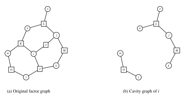
, with an edge between i and I if and only if i∈I, that is, if xi participates in the factorψI. We will represent factor nodes visually as rectangles and variable nodes as circles. See Figure 1(a) for an example of a factor graph. We denote the neighboring nodes of a variable node i by Ni:={I∈F
: i∈I}and the neighboring nodes of a factor node I simply by I={i∈V
: i∈I}. Further, we define for each variable i∈V
the set∆i :=SNiconsisting of all variables that appear in some factor in which variable i participates, and the set∂i :=∆i\ {i}, the Markov blanket of i.
i
j
k
l m
n
o
I
J K
L
M
O
(a) Original factor graph
j
k
l m
n
o
L
M
O
(b) Cavity graph of i
Figure 1: (a) Original factor graph, corresponding to the probability distribution P(x) =
1
ZψL(xj,xn,xo)ψI(xi,xj)ψM(xj,xk)ψK(xi,xm,xn)ψJ(xi,xk,xl)ψO(xl,xm); (b) Factor graph corresponding to the cavity network of variable i, obtained by removing variable i and the factor nodes that contain i (i.e., I, J and K). The Markov blanket of i is∂i={j,k,l,m,n}. The cavity distribution Z\i(x∂i)is the (unnormalized) marginal on x∂i of the probability distribution corresponding to the cavity graph (b).
indices. For convenience, we will define for any subset
A
⊂F
the product of the corresponding factors:ΨA(xSA):=
∏
I∈A
ψI(xI).
2.2 Cavity Networks and Loop Corrections
The notion of a cavity stems from statistical physics, where it was used originally to calculate properties of random ensembles of certain graphical models (M´ezard et al., 1987). A cavity is obtained by removing one variable from the graphical model, together with all the factors in which that variable participates.
In our context, we define cavity networks as follows (see also Figure 1):
Definition 2.1 Given a graphical model(
V
,F
,{ψI}I∈F)and a variable i∈V
, the cavity network of variable i is the graphical model(V
\i,F
\Ni,{ψI}I∈F\Ni).The probability distribution corresponding to the cavity network of variable i is thus proportional to:
Ψ\Ni(x\i) =
∏
I∈Fi6∈I
ψI(xI).
Definition 2.2 Given a graphical model(
V
,F
,{ψI}I∈F)and a variable i∈V
, the cavitydistri-bution of i is
Z\i(x∂i):=
∑
x\∆i
Ψ\Ni(x\i). (2)
Thus the cavity distribution of i is proportional to the marginal of the cavity network of i on the Markov blanket∂i. The cavity distribution describes the effective interactions (or correlations) in-duced by the cavity network on the neighbors∂i of variable i. Indeed, from Equations (1) and (2) and the trivial observation thatΨF =ΨNiΨ\Ni we conclude:
P(x∆i)∝Z\i(x∂i)ΨNi(x∆i). (3)
Thus, given the cavity distribution Z\i(x∂i), one can calculate the marginal distribution of the original graphical model P on x∆i, provided that the cardinality of
X
∆iis not too large.In practice, exact cavity distributions are not known, and the only way to proceed is to use approximate cavity distributions. Given some approximate inference method (e.g., BP), there are two ways to calculate P(x∆i): either use the method to approximate P(x∆i) directly, or use the method to approximate Z\i(x∂i) and use Equation (3) to obtain an approximation to P(x∆i). The latter approach generally gives more accurate results, since the complexity of the cavity network is less than that of the original network. In particular, the cavity network of variable i contains no loops involving that variable, since all factors in which i participates have been removed (e.g., the loop i−J−l−O−m−K−i in the original network, Figure 1(a), is not present in the cavity network, Figure 1(b)). Thus the latter approach to calculating P(x∆i) takes into account loops involving variable i, although in an approximate way. It does not, however, take into account the other loops in the original graphical model. The basic idea of the loop correction approach of Montanari and Rizzo (2005) is to use the latter approach for all variables in the network, but to adjust the approximate cavity distributions in order to cancel out approximation errors before (3) is used to obtain the final approximate marginals. This approach takes into account all the loops in the original network, in an approximate way.
This basic idea can be implemented in several ways. Here we propose an implementation which we will show to have certain advantages over the original implementation proposed in Montanari and Rizzo (2005). In particular, it is directly applicable to arbitrary factor graphs with variables taking an arbitrary (discrete) number of values and factors that may contain zeroes and consist of an arbitrary number of variables. In the remaining subsections, we will first discuss our proposed implementation in detail. In Section 2.6 we will discuss differences with the original approach.
2.3 Combining Approximate Cavity Distributions to Cancel Out Errors
Suppose that we have obtained an initial approximationζ\0i(x∂i)of the (exact) cavity distribution Z\i(x∂i), for each i∈
V
. Let i∈V
and consider the approximation error of the cavity distribution of i, that is, the exact cavity distribution of i divided by its approximation:Z\i(x∂i)
ζ\i 0(x∂i)
In general, this is an arbitrary function of the variables x∂i. However, for our purposes, we approxi-mate the error as a product of factors defined on small subsets of∂i in the following way:
Z\i(x∂i)
ζ\i 0(x∂i)
≈
∏
I∈Niφ\i I (xI\i).
Thus we assume that the approximation error lies near a submanifold parameterized by the error factors{φ\Ii(xI\i)}I∈Ni. If we were able to calculate these error factors, we could improve our initial approximationζ\0i(x∂i)by replacing it with the product
ζ\i(x
∂i):=ζ\
i
0(x∂i)
∏
I∈Niφ\i
I (xI\i)≈Z\i(x∂i). (4)
Using (3), this would then yield an improved approximation of P(x∆i).
It turns out that the error factors can indeed be calculated by exploiting the redundancy of the in-formation in the initial cavity approximations{ζ\0i}i∈V. The fact that allζ\iprovide approximations to marginals of the same probability distribution P(x)via (3) can be used to obtain consistency con-straints. The number of constraints obtained in this way is usually enough to solve for the unknown error factors{φ\Ii(xI\i)}i∈V,I∈Ni.
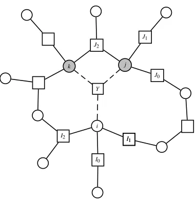
Here we propose the following consistency constraints. Let Y ∈
F
, i∈Y and j∈Y with i6= j (see also Figure 2). Consider the graphical model(V
,F
\Y,{ψI}I∈F\Y)that is obtained from the original graphical model by removing factorψY. The product of all factors (exceptψY) obviously satisfies:Ψ\Y =ΨNi\YΨ\Ni=ΨNj\YΨ\Nj.
Using (2) and summing over all xkfor k6∈Y\i, we obtain the following equation, which holds for the exact cavity distributions Z\iand Z\j:
∑
xi
∑
x∆i\Y
ΨNi\YZ\ i=
∑
xi
∑
x∆j\Y
ΨNj\YZ\ j.
Substituting our basic assumption (4) on both sides and pulling the factor φY\i(xY\i) in the l.h.s. through the summation, we obtain:
φ\i Y
∑
xi
∑
x∆i\Y
ΨNi\Yζ
\i
0
∏
I∈Ni\Y
φ\i I =
∑
xi
∑
x∆j\Y
ΨNj\Yζ
\j
0
∏
J∈Nj
φ\j J .
Since this should hold for each j∈Y\i, we can take the geometric mean of the r.h.s. over all j∈Y\i. After rearranging, this yields:
φ\i Y =
∏
j∈Y\i
∑
xi x∑
∆j\YΨNj\Yζ
\j
0
∏
J∈Nj
φ\j J
!1/|Y\i|
∑
xi
∑
x∆i\Y
ΨNi\Yζ
\i
0
∏
I∈Ni\Y
φ\i I
for all i∈
V
, Y ∈Ni. (5)I0
I1
I1
I2
J0
J1
J2
Y
i j k
Figure 2: Part of the factor graph, illustrating the derivation of (5). The two gray variable nodes correspond to Y\i={j,k}.
Solving the consistency Equations (5) simultaneously for the error factors{φ\Ii}i∈V,I∈Ni can be done using a simple fixed point iteration algorithm, for example, Algorithm 1. The input consists of the initial approximations{ζ\0i}i∈V to the cavity distributions. It calculates the error factors that satisfy (5) by fixed point iteration and from the fixed point, it calculates improved approximations of the cavity distributions{ζ\i}i∈V using Equation (4).1 From the improved cavity distributions, the loop-corrected approximations to the single-variable marginals of the original probability distribu-tion (1) can be calculated as follows:
Pi(xi)≈bi(xi)∝
∑
x∂iΨNi(x∆i)ζ\ i(x
∂i), (6)
where the factorψY is now included. Algorithm 1 uses a sequential update scheme, but other update schemes are possible (e.g., random sequential or parallel). In practice, the fixed sequential update scheme often converges without the need for damping.
Alternatively, one can formulate Algorithm 1 in terms of the “beliefs”
Qi(x∆i)∝ ΨNi(x∆i)ζ
\i
0(x∂i)
∏
I∈Niφ\i
I (xI\i) =ΨNi(x∆i)ζ\ i(x
∂i). (7)
As one easily verifies, the update equation
Qi←Qi
∏
j∈Y\i x∆
∑
j\(Y\i)QjψY−1
!1/|Y\i|
∑
x∆i\(Y\i)
QiψY−1
Algorithm 1 Loop Correction Algorithm
Input: initial approximate cavity distributions{ζ\0i}i∈V
Output: improved approximate cavity distributions{ζ\i}i∈V
1: repeat
2: for all i∈
V
do3: for all Y∈Nido
4: φ\Yi(xY\i)←
∏
j∈Y\i
∑
xi∑
x∆j\Y
ΨNj\Yζ
\j
0
∏
J∈Nj
φ\j J
!1/|Y\i|
∑
xi
∑
x∆i\Y
ΨNi\Yζ
\i
0
∏
I∈Ni\Y
φ\i I
5: end for
6: end for
7: until convergence
8: for all i∈
V
do9: ζ\i(x∂i)←ζ0\i(x∂i)∏I∈Niφ
\i I (xI\i)
10: end for
is equivalent to line 1 of Algorithm 1. Intuitively, the update improves the approximate distribution Qion∆i by replacing its marginal on Y\i (in the absence of Y ) by a more accurate approximation of this marginal, namely the numerator. Written in this form, the algorithm is reminiscent of iterative proportional fitting (IPF). However, contrary to IPF, the desired marginals are also updated at each iteration. Note that after convergence, the large beliefs Qi(x∆i) need not be consistent, that is, in general∑x∆i\JQi6=∑x∆j\JQjfor i,j∈
V
, J⊆∆i∩∆j.2.4 A Special Case: Factorized Cavity Distributions
In the previous subsection we have discussed how to improve approximations of cavity distribu-tions. We now discuss what happens when we use the simplest possible initial approximations {ζ\0i}i∈V, namely constant functions, in Algorithm 1. This amounts to the assumption that no loops
are present. We will show that if the factor graph does not contain short loops consisting of four nodes, fixed points of the standard BP algorithm are also fixed points of Algorithm 1. In this sense, Algorithm 1 can be considered to be a generalization of the BP algorithm. In fact, this holds even if the initial approximations factorize in a certain way, as will be shown below.
If all factors involve at most two variables, one can easily arrange for the factor graph to have no loops of four nodes. See Figure 1(a) for an example of a factor graph which has no loops of four nodes. The factor graph depicted in Figure 2 does have a loop of four nodes: k−Y−j−J2−k.
Theorem 2.1 If the factor graph corresponding to (1) has no loops of exactly four nodes, and all
initial approximate cavity distributions factorize in the following way:
ζ\i
0(x∂i) =
∏
I∈Niξ\i
I (xI\i) ∀i∈
V
, (8)Proof Note that replacing the initial cavity approximations by
ζ\i
0(x∂i)7→ζ\ i
0(x∂i)
∏
I∈Niε\i I (xI\i)
for arbitrary positive functionsε\Ii(xI\i)does not change the beliefs (7) corresponding to the fixed points of (5). Thus, without loss of generality, we can assumeζ\0i(x∂i) =1 for all i∈
V
. The BP update equations are (Kschischang et al., 2001):µj→I(xj)∝
∏
J∈Nj\IµJ→j(xj) j∈
V
,I∈Nj,µI→i(xi) ∝
∑
xI\iψI(xI)
∏
j∈I\iµj→I(xj) I∈
F
,i∈I(9)
in terms of messages{µJ→j(xj)}j∈V,J∈Nj and{µj→J(xj)}j∈V,J∈Nj. Assume that the messages µ are a fixed point of (9) and take the Ansatz
φ\i
I (xI\i) =
∏
k∈I\iµk→I(xk) for i∈
V
,I∈Ni.Then, for i∈
V
, Y ∈Ni, j∈Y\i, we can write out part of the numerator of (5) as follows:∑
xi
∑
x∆j\Y
ΨNj\Yζ
\j
0
∏
J∈Nj
φ\j J =
∑
xi
∑
x∆j\Y
φ\j Y
∏
J∈Nj\Y
ψJφ\Jj
=
∑
xi
∏
k∈Y\j µk→Y
!
∏
J∈Nj\Y
∑
xJ\j
ψJ
∏
k∈J\jµk→J
=
∑
xi
∏
k∈Y\j µk→Y
!
µj→Y =
∑
xi∏
k∈Y
µk→Y∝
∏
k∈Y\iµk→Y
=φ\Yi,
where we used the BP update Equations (9) and rearranged the summations and products using the assumption that the factor graph has no loops of four nodes. Thus, the numerator of the r.h.s. of (5) is simplyφY\i. Using a similar calculation, one can derive that the denominator of the r.h.s. of (5) is constant, and hence (5) is valid (up to an irrelevant constant).
For Y ∈
F
, i∈Y , the marginal on xY of the belief (7) can be written in a similar way:∑
x∆i\Y
Qi∝
∑
x∆i\YΨNi
∏
I∈Niφ\i I =
∑
x∆i\YI
∏
∈NiψI
∏
k∈I\iµk→I
=ψY
∏
k∈Y\iµk→Y
!
∏
I∈Ni\Y
∑
xI\i
ψI
∏
k∈I\iµk→I
=ψY
∏
k∈Y\iµk→Y
!
∏
I∈Ni\Y
µI→i=ψY
∏
k∈Y\iµk→Y
!
µi→Y
=ψY
∏
k∈Ywhich is proportional to the BP belief bY(xY)on xY. Hence, also the single-variable marginal bi de-fined in (6) corresponds to the BP single-variable belief, since both are marginals of bY for Y∈Ni.
If the factor graph does contain loops of four nodes, we usually observe that the fixed point of Algorithm 1 coincides with the solution of the “minimal” CVM approximation when using factor-ized initial cavity approximations as in (8). The minimal CVM approximation uses all maximal factors as outer clusters (a maximal factor is a factor defined on a domain which is not a strict subset of the domain of another factor). In that case, the factor beliefs found by Algorithm 1 are consis-tent, that is,∑x∆i
\YQi=∑x∆j\YQj for i,j∈Y , and are identical to the minimal CVM factor beliefs. In particular, this holds for all the graphical models used in Section 3.2
2.5 Obtaining Initial Approximate Cavity Distributions
There is no principled way to obtain the initial cavity approximations ζ\0i(x∂i). In the previous subsection, we investigated the results of applying the LC algorithm on factorizing initial cavity approximations. More sophisticated approximations that do take into account the effect of loops can significantly enhance the accuracy of the final result. Here, we will describe one method, which uses BP on clamped cavity networks. This method captures all interactions in the cavity distribution of i in an approximate way and can lead to very accurate results. Instead of BP, any other approximate inference method that gives an approximation of the normalizing constant Z in (1) can be used, such as mean field, TreeEP (Minka and Qi, 2004), a double-loop version of BP (Heskes et al., 2003) which has guaranteed convergence towards a minimum of the Bethe free energy, or some variant of GBP (Yedidia et al., 2005). One could also choose the method for each cavity separately, trading accuracy versus computation time. We focus on BP because it is a very fast and often relatively accurate algorithm.
Let i∈
V
and consider the cavity network of i. For each possible state of x∂i, run BP on the cavity network clamped to that state x∂iand calculate the corresponding Bethe free energy F\i Bethe(x∂i) (Yedidia et al., 2005). Then, take the following initial approximate cavity distribution:
ζ\i
0(x∂i)∝e−F \i Bethe(x∂i).
This procedure is exponential in the size of∂i: it uses∏j∈∂i
X
j
BP runs. However, many networks
encountered in applications are relatively sparse and have limited cavity size and the computational cost may be acceptable.
This particular way of obtaining initial cavity distributions has the following interesting prop-erty: in case the factor graph contains only a single loop and assuming that the fixed point is unique, the final beliefs (7) resulting from Algorithm 1 are exact. This can be shown using an argument similar to that given in Montanari and Rizzo (2005). Suppose that the graphical model contains exactly one loop and let i∈
V
. First, consider the case that i is part of the loop; removing i will break the loop and the remaining cavity network will be singly connected. The cavity distribution approximated by BP will thus be exact. Now if i is not part of the loop, removing i will divide thenetwork into several connected components, one for each neighbor of i. This implies that the cav-ity distribution calculated by BP contains no higher-order interactions, that is,ζ\0i is exact modulo single-variable interactions. Because the final beliefs (7) are invariant under perturbation of theζ\0i by single-variable interactions, the final beliefs calculated by Algorithm 1 are exact if the fixed point is unique.
If all interactions are pairwise and each variable is binary and has exactly|∂i|=d neighbors, the time complexity of the resulting “loop-corrected BP” (LCBP) algorithm is given by
O
(N2dEIBP+Nd2d+1ILC), where E is the number of edges in the factor graph, IBP is the average number of iterations of BP on a clamped cavity network and ILC is the number of iterations needed to obtain convergence in Algorithm 1.
2.6 Differences with the Original Implementation
As mentioned before, the idea of estimating the cavity distributions and imposing certain consis-tency relations amongst them has been first presented in Montanari and Rizzo (2005). In its simplest form (i.e., the so-called first-order correction), the implementation of that basic idea as proposed by Montanari and Rizzo (2005) differs from our proposed implementation in the following aspects.
First, the original method described by Montanari and Rizzo (2005) is only formulated for the rather special case of binary variables and pairwise interactions. In contrast, our method is formulated in a general way that makes it applicable to factor graphs with variables having more than two possible values and factors consisting of more than two variables. Also, factors may contain zeroes. The generality that our implementation offers is important for many practical applications. In the rest of this section, we will assume that the graphical model (1) belongs to the special class of models with binary variables with pairwise interactions, allowing further comparison of both implementations.
An important difference is that Montanari and Rizzo (2005) suggest to deform the initial ap-proximate cavity distributions by altering certain cumulants (also called “connected correlations”), instead of altering certain interactions. In general, for a set
A
of ±1-valued random variables {xi}i∈A, one can define for any subsetB
⊆A
the momentMB :=
∑
xA
P(xA)
∏
j∈B
xj.
The moments{MB}B⊆Aare a parameterization of the probability distribution P(xA). An alternative parameterization is given in terms of the cumulants. The (joint) cumulants {CE}E⊆A are certain
polynomials of the moments, defined implicitly by the following equations:
MB =
∑
C∈Part(B)E
∏
∈CCE
where Part(
B
) is the set of partitions ofB
.3 In particular, Ci=Mi and Ci j =Mi j−MiMj for all i,j∈A
with i6= j. Montanari and Rizzo (2005) propose to approximate the cavity distributions by estimating the pair cumulants and assuming higher-order cumulants to be zero. Then, the singleton cumulants (i.e., the single-variable marginals) are altered, keeping higher-order cumulants fixed, in3. For a set X , a partition of X is a nonempty set Y such that each Z∈Y is a nonempty subset of X andS
such a way as to impose consistency of the single-variable marginals, in the absence of interac-tions shared by two neighboring cavities. We refer the reader to Appendix A for a more detailed description of the implementation in terms of cumulants suggested by Montanari and Rizzo (2005). The assumption suggested in Montanari and Rizzo (2005) that higher-order cumulants are zero is the most important difference with our method, which instead takes into account effective in-teractions in the cavity distribution of all orders. In principle, the cumulant parameterization also allows for taking into account higher-order cumulants, but this would not be very efficient due to the combinatorics needed for handling the partitions.
A minor difference lies in the method to obtain initial approximations to the cavity distributions. Montanari and Rizzo (2005) propose to use BP in combination with linear response theory to obtain the initial pairwise cumulants. This difference is not very important, since one could also use BP on clamped cavity networks instead, which turns out to give almost identical results.
As we will show in Section 3, our method of altering interactions appears to be more robust and still works in regimes with strong interactions, whereas the cumulant implementation suffers from convergence problems for strong interactions.
Montanari and Rizzo (2005) also derive a linearized version of their cumulant-based scheme (by expanding up to first order in terms of the pairwise cumulants, see Appendix A) which is quadratic in the size of the cavity. This linearized, cumulant-based version is currently the only one that can be applied to networks with large Markov blankets (cavities), that is, where the maximum number of states maxi∈V|
X
∆i|is large, provided that all variables are binary and interactions are pairwise.3. Numerical Experiments
We have performed various numerical experiments to compare the quality of the results and the computation time of the following approximate inference methods:
MF Mean field, with a random sequential update scheme and no damping.
BP Belief propagation. We have used the recently proposed update scheme (Elidan et al., 2006),
which converges also for difficult problems without the need for damping.
TreeEP TreeEP (Minka and Qi, 2004), without damping. We generalized the method of choosing
the base tree described in Minka and Qi (2004) to multiple variable factors as follows: when estimating the mutual information between xiand xj, we take the product of the marginals on {i,j} of all the factors that involve xi and/or xj. Other generalizations of TreeEP to higher-order factors are possible (e.g., by clustering variables), but it is not clear how to do this in general in an optimal way.
LCBP (“Loop-corrected belief propagation”) Algorithm 1, where the approximate cavities are
ini-tialized according to the description in Section 2.5.
LCBP-Cum The original cumulant-based loop correction scheme by Montanari and Rizzo (2005),
valid interval in the hope that the method will converge to a valid result, which it sometimes does.
LCBP-Cum-Lin Similar to LCBP-Cum, but instead of the full update Equations (14), the
lin-earized update Equations (15) are used.
CVM-Min A double-loop implementation (Heskes et al., 2003) of the minimal CVM
approxima-tion, which uses (maximal) factors as outer clusters.
CVM-∆ A double-loop implementation of CVM using the sets{∆i}i∈V as outer clusters. These are the same sets of variables as used by LCBP (c.f. (7)) and therefore it is interesting to compare both algorithms.
CVM-Loopk A double-loop implementation of CVM, using as outer clusters all (maximal) factors
together with all loops in the factor graph that consist of up to k different variables (for k=
3,4,5,6,8).
We have used a double-loop implementation of CVM instead of GBP because the former is guaranteed to converge to a local minimum of the Kikuchi free energy (Heskes et al., 2003) without damping, whereas the latter often only converges with strong damping. The difficulty with damping is that the optimal damping constant is not known a priori, which necessitates multiple trial runs with different damping constants, until a suitable one is found. Using too much damping slows down convergence, whereas a certain amount of damping is required to obtain convergence in the first place. Therefore, in general we expect that (damped) GBP is not much faster than a double-loop implementation because of the computational cost of finding the optimal damping constant.
To be able to assess the errors of the various approximate methods, we have only considered problems for which exact inference (using a standard JunctionTree method) was still feasible.
For each approximate inference method, we report the maximum `∞error of the approximate single-variable marginals bi, calculated as follows:
Error :=max i∈V maxxi∈Xi|
bi(xi)−P(xi)|
where P(xi)is the exact marginal calculated using the JunctionTree method.
The computation time was measured as CPU time in seconds on a 2.4 GHz AMD Opteron 64bits processor with 4 GB memory. The timings should be seen as indicative because we have not spent equal amounts of effort optimizing each method.4
We consider an iterative method to be “converged” after T time steps if for each variable i∈
V
, the`∞distance between the approximate probability distributions of that variable at time step T and T+1 is less thanε=10−9.We have studied four different model classes: (i) random graphs of uniform degree with pair-wise interactions and binary variables; (ii) random factor graphs with binary variables and factor nodes of uniform degree k=3; (iii) the ALARM network, which has variables taking on more than two possible values and factors consisting of more than two variables; (iv) PROMEDAS networks, which have binary variables but factors consisting of more than two variables. For more extensive experiments, see Mooij and Kappen (2006).
3.1 Random Regular Graphs with Binary Variables
We have compared various approximate inference methods on random graphs, consisting of N bi-nary (±1-valued) variables, having only pairwise interactions, where each variable has the same degree|∂i|=d. In this case, the probability distribution (1) can be written in the following way:
P(x) = 1
Zexp i
∑
∈V
θixi+ 1 2i
∑
∈Vj
∑
∈∂i Ji jxixj!
.
The parameters{θi}i∈V are called the local fields and the parameters{Ji j =Jji}i∈V,j∈∂iare called the couplings. The graph structure and the parametersθand J were drawn randomly for each in-stance. The local fields{θi}were drawn independently from a
N
(0,βΘ)distribution (i.e., a normal distribution with mean 0 and standard deviationβΘ). For the couplings{Ji j}, we took mixed (“spin-glass”) couplings, drawn independently from a normal distribution Ji j ∼N
0,βtanh−1√1
d−1
. The constantβ(called “inverse temperature” in statistical physics) controls the overall interaction strength and thereby the difficulty of the inference problem, largerβcorresponding usually to more difficult problems. The constant Θcontrols the relative strength of the local fields, where larger
Θresult in easier inference problems. The particular d-dependent scaling of the couplings is used in order to obtain roughly d-independent behavior. ForΘ=0 and for β≈1, a phase transition occurs in the limit of N→∞, going from an easy “paramagnetic” phase forβ<1 to a complicated “spin-glass” phase forβ>1.5
We have also done experiments with positive (“attractive” or “ferromagnetic”) couplings, but the conclusions from these experiments did not differ significantly from those using mixed couplings (Mooij and Kappen, 2006). Therefore we do not report those experiments here.
3.1.1 N=100, d=3, STRONGLOCALFIELDS(Θ=2)
We have studied various approximate inference methods on regular random graphs of low degree d=3, consisting of N =100 variables, with relatively strong local fields of strengthΘ=2. We have considered various overall interaction strengthsβbetween 0.01 and 10. For each value ofβ, we have used 16 random instances. On each instance, we have run various approximate inference algorithms.
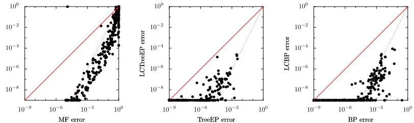
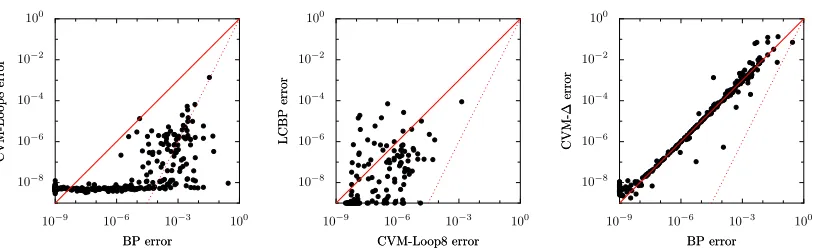
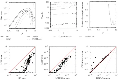
Figure 3 shows results for MF, BP and TreeEP, and their loop-corrected versions, LCMF, LCBP and LCTreeEP. The loop-corrected versions are the result of Algorithm 1, initialized with approx-imate cavity distributions obtained by the procedure described in Section 2.5 (using MF, BP, and TreeEP in the role of BP). Note that the loop correction method significantly reduces the error in each case. In fact, on average the loop-corrected error is approximately given by the square of the uncorrected error, as is apparent from the scatter plots in Figure 4. BP is the fastest of the uncor-rected methods and TreeEP is the most accurate but also the slowest uncoruncor-rected method. MF is both slower and less accurate than BP. Unsurprisingly, the loop-corrected methods show similar relative performance behaviors. Because BP is very fast and relatively accurate, we focus on LCBP in the rest of this article. Note further that although the graph is rather sparse, the improvement of LCBP over BP is significantly more than the improvement of TreeEP over BP.
5. More precisely, the PA-SG phase transition occurs atΘ=0 and(d−1) =
tanh2(βJi j)
10−8 10−6 10−4 10−2 100
Max.
error
Max.
error
0.01 0.1 1 10
β β
10−2 100 102 104
Time
(
s
)
Time
(
s
)
0.01 0.1 1 10
β β
MF
BP
TreeEP
LCMF
LCBP
LCTreeEP
Figure 3: Error (left) and computation time (right) as a function of interaction strength for vari-ous approximate inference methods (MF, BP, TreeEP) and their loop-corrected versions (LCMF, LCBP, LCTreeEP). The averages (calculated in the logarithmic domain) were computed from the results for 16 randomly generated instances of(N=100,d=3) reg-ular random graphs with strong local fieldsΘ=2.
10−8 10−6 10−4 10−2 100
LCMF
error
LCMF
error
10−9 10−6 10−3 100
MF error MF error
10−8
10−6
10−4
10−2
100
LCT
reeEP
error
LCT
reeEP
error
10−9 10−6 10−3 100
TreeEP error TreeEP error
10−8
10−6
10−4
10−2
100
LCBP
error
LCBP
error
10−9 10−6 10−3 100
BP error BP error
Figure 4: Pairwise comparisons of errors of uncorrected and loop-corrected methods, for the same instances as in Figure 3. The solid red lines correspond with y=x, the dotted red lines with y=x2. Only the cases have been plotted for which both approximate inference meth-ods have converged. Saturation of errors around 10−9is an artifact due to the convergence criterion.
10−8 10−6 10−4
10−2 100
Max.
error
Max.
error
0.01 0.1 1 10
β β
0.001
0.01
0.1
1 10 Time ( s ) Time ( s )
0.01 0.1 1 10
β β 0 0.25 0.5 0.75 1 F raction of con v erged instances F raction of con v erged instances
0.01 0.1 1 10
β β
BP LCBP-Cum-Lin LCBP-Cum LCBP
Figure 5: For the same instances as in Figure 3: average error (left), average computation time (center) and fraction of converged instances (right) as a function of interaction strengthβ for various variants of the LC method. The averages of errors and computation time were calculated from the converged instances only. The average computation time and fraction of converged instances for LCBP-Cum and LCBP-Cum-Lin are difficult to distinguish, because they are (almost) identical.
10−8
10−6
10−4
10−2
100
LCBP-Cum
error
LCBP-Cum
error
10−9 10−6 10−3 100
BP error BP error
10−8
10−6
10−4
10−2
100
LCBP-Cum-Lin
error
LCBP-Cum-Lin
error
10−9 10−6 10−3 100
LCBP-Cum error LCBP-Cum error
10−8
10−6
10−4
10−2
100
LCBP
error
LCBP
error
10−9 10−6 10−3 100
LCBP-Cum error LCBP-Cum error
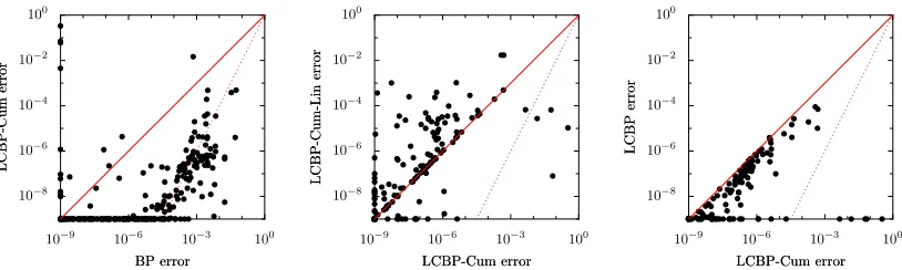
Figure 6: Pairwise comparisons of errors of various methods for the same instances as in Figure 3. Only the cases have been plotted for which both approximate inference methods con-verged.
We speculate that the reason for the break-down of LCBP-Cum and LCBP-Cum-Lin for strong interactions is due to the choice of cumulants instead of interactions. Indeed, consider two random variables x1 and x2 with fixed pair interaction exp(Jx1x2). By altering the singleton interactions exp(θ1x1) and exp(θ2x2), one can obtain any desired marginals of x1 and x2. However, a fixed pair cumulant C12 =hx1x2i − hx1ihx2i imposes a constraint on the range of possible expectation values hx1iandhx2i (hence on the single-variable marginals of x1and x2); the freedom of choice in these marginals becomes less as the pair cumulant becomes stronger. We believe that something similar happens for LCBP-Cum (and LCBP-Cum-Lin): for strong interactions, the approximate pair cumulants in the cavity are strong, and even tiny errors can lead to inconsistencies which prevent convergence.
10−8
10−6
10−4
10−2
100
Max.
error
Max.
error
0.01 0.1 1 10
β β
0.001 0.01 0.1 1 10 100
Time
(
s
)
Time
(
s
)
0.01 0.1 1 10
β β
BP CVM-∆ CVM-Loop4 CVM-Loop6 CVM-Loop8 LCBP
Figure 7: Average errors (left) and computation times (right) for various CVM methods (and LCBP, for reference) on the same instances as in Figure 3. All methods converged on all in-stances.
10−8 10−6 10−4 10−2 100
CVM-Lo
op8
error
CVM-Lo
op8
error
10−9 10−6 10−3 100 BP error
BP error
10−8 10−6 10−4 10−2 100
LCBP
error
LCBP
error
10−9 10−6 10−3 100 CVM-Loop8 error CVM-Loop8 error
10−8
10−6
10−4
10−2
100
CVM-∆
error
CVM-∆
error
10−9 10−6 10−3 100
BP error BP error
Figure 8: Pairwise comparisons of errors for various methods for the same instances as in Figure 3.
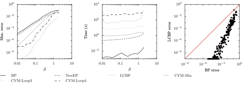
on BP. Furthermore, as expected, the use of larger clusters (that subsume longer loops) improves the results, although computation time quickly increases. CVM-Loop3 (not plotted) turned out not to give any improvement over BP, simply because there were (almost) no loops of 3 variables present. The most accurate CVM method, CVM-Loop8, needs more computation time than LCBP, whereas it yields inferior results.6
In addition to the CVM-Loop methods, we compared with the CVM-∆ method, which uses {∆i}i∈V as outer clusters. These clusters subsume the clusters used implicitly by BP (which are simply the pairwise factors) and therefore one would naively expect that the CVM-∆approximation yields better results. Surprisingly however, the quality of CVM-∆is similar to that of BP, although its computation time is enormous. This illustrates that simply using larger clusters for CVM does not always lead to better results. Furthermore, we conclude that although LCBP and CVM-∆use identical clusters to approximate the target probability distribution, the nature of both approxima-tions is very different.
10−8 10−6 10−4 10−2 100
Max.
error
Max.
error
0.01 0.1 1 10
β β 0.001 0.01 0.1 1 10 100 Time ( s ) Time ( s )
0.01 0.1 1 10
β β
0 0.25 0.5 0.75 1 F raction of con v erged instances F raction of con v erged instances
0.01 0.1 1 10
β β
BP TreeEP LCBP-Cum-Lin LCBP-Cum
LCBP CVM-Loop4
10−8 10−6 10−4 10−2 100 LCBP error LCBP error
10−9 10−6 10−3 100
BP error BP error
10−8 10−6 10−4 10−2 100 LCBP error LCBP error
10−9 10−6 10−3 100
LCBP-Cum error LCBP-Cum error
10−8
10−6
10−4
10−2
100
LCBP-Cum-Lin
error
LCBP-Cum-Lin
error
10−9 10−6 10−3 100
LCBP-Cum error LCBP-Cum error
Figure 9: Selected results for(N=50,d=6)regular random graphs with strong local fieldsΘ=2. The averaged results for LCBP-Cum and LCBP-Cum-Lin nearly coincide forβ.1.
3.1.2 WEAKLOCALFIELDS(Θ=0.2)
We have done the same experiments also for weak local fields (Θ=0.2), with the other parameters unaltered (i.e., N =100, d=3). The picture roughly remains the same, apart from the following differences. First, the influence of the phase transition is more pronounced; many methods have severe convergence problems aroundβ=1. Second, the negative effect of linearization on the error (LCBP-Cum-Lin compared to LCBP-Cum) is smaller.
3.1.3 LARGERDEGREE(d=6)
To study the influence of the degree d=|∂i|, we have done additional experiments for d=6. We had to reduce the number of variables to N=50, because exact inference was infeasible for larger values of N due to quickly increasing treewidth. The results are shown in Figure 9. As in the previous experiments, BP is the fastest and least accurate method, whereas LCBP yields the most accurate results, even for highβ. Again we see that the LCBP error is approximately the square of the BP error and that LCBP gives better results than LCBP-Cum, but needs more computation time. However, we also note the following differences with the case of low degree (d =3). The relative improvement of TreeEP over BP has decreased. This could have been expected, because in denser networks, the effect of taking out a tree becomes less.
10−9 10−6 10−3 100
Max.
error
Max.
error
10 20 50
N N
10−2 100 102 104
Time
(
s
)
Time
(
s
)
10 20 50
N N
BP TreeEP LCBP LCBP-Cum LCBP-Cum-Lin CVM-Loop3 CVM-Loop4 JunctionTree
Figure 10: Error (left) and computation time (right) as a function of N (the number of variables), for random graphs with uniform degree d=6,β=0.1 andΘ=2. Points are averages over 16 randomly generated instances. Each method converged on all instances. The results for LCBP-Cum and LCBP-Cum-Lin coincide.
increased and it is the slowest of all methods. We decided to abort the calculations for CVM-Loop6 and CVM-Loop8, because computation time was prohibitive due to the enormous amount of short loops present. We conclude that the CVM-Loop approach to loop correction is not very efficient if there are many loops present.
Surprisingly, the results of LCBP-Cum-Lin are now very similar in quality to the results of LCBP-Cum, except for a few isolated cases (presumably on the edge of the convergence region).
3.1.4 SCALING WITHN
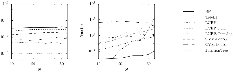
We have investigated how computation time and error scale with the number of variables N, for fixedβ=0.1,Θ=2 and d=6. We used a machine with more memory (16 GB) to be able to do exact inference without swapping also for N=60. The results are shown in Figure 10. The error of each method is approximately constant.
BP computation time should scale approximately linearly in N, which is difficult to see in this plot. LCBP variants are expected to scale quadratic in N (since d is fixed) which we have verified by checking the slopes of corresponding lines in the plot for large values of N. The computation time of CVM-Loop3 and CVM-Loop4 seems to be approximately constant, probably because the large number of overlaps of short loops for small values of N causes difficulties. The computation time of the exact JunctionTree method quickly increases due to increasing treewidth; for N=60 it is already ten times larger than the computation time of the slowest approximate inference method.
We conclude that for large N, exact inference is infeasible, whereas LCBP still yields very accurate results using moderate computation time.
3.1.5 SCALING WITHd
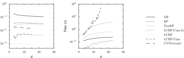
It is also interesting to see how various methods scale with d, the variable degree, which is directly related to the cavity size. We have done experiments for random graphs of size N=24 with fixed
10−9 10−6
10−3 100
Max.
error
Max.
error
0 10 20 30
d d
10−2 100 102 104
Time
(
s
)
Time
(
s
)
0 10 20 30
d d
MF BP TreeEP LCBP-Cum-Lin LCBP LCBP-Cum CVM-Loop3
Figure 11: Error (left) and computation time (right) as a function of variable degree d for regular random graphs of N=24 variables for β=0.1 and Θ=2. Points are averages over 16 randomly generated instances. Each method converged on all instances. Errors of LCBP-Cum and LCBP-Cum-Lin coincide for d≤15; for d>15, LCBP-Cum became too slow.
Due to the particular dependence of the interaction strength on d, the errors of most methods depend only slightly on d. TreeEP is an exception: for larger d, the relative improvement of TreeEP over BP diminishes, and the TreeEP error approaches the BP error. CVM-Loop3 gives better quality, but needs relatively much computation time and becomes very slow for large d due to the large increase in the number of loops of 3 variables. LCBP is the most accurate method, but becomes very slow for large d. LCBP-Cum is less accurate and becomes slower than LCBP for large d, because of the additional overhead of the combinatorics needed to perform the update equations. The accuracy of LCBP-Cum-Lin is indistinguishable from that of LCBP-Cum, although it needs significantly less computation time.
Overall, we conclude from Section 3.1 that for these binary, pairwise graphical models, LCBP is the best method for obtaining high accuracy marginals if the graphs are sparse, LCBP-Cum-Lin is the best method if the graphs are dense and LCBP-Cum shows no clear advantages over either method.
3.2 Multi-variable Factors
We now go beyond pairwise interactions and study a class of random factor graphs with binary variables and uniform factor degree |I|=k (for all I∈
F
) with k>2. The number of variables is N and the number of factors is M. The factor graphs are constructed by starting from an empty graphical model(V
,/0,/0)and adding M random factors, where each factor is obtained in the follow-ing way: a subset I={I1, . . . ,Ik} ⊆V
of k different variables is drawn; a vector of 2k independent random numbers{JI(xI)}xI∈XI is drawn from aN
(0,β)distribution; the factorψI(xI):=exp JI(xi) is added to the graphical model. We only use those constructed factor graphs that are connected.7 The parameterβagain controls the interaction strength.We have done experiments for (N=50,M=50,k=3)for various values of βbetween 0.01 and 2. For each value ofβ, we have used 16 random instances. For higher values ofβ, computation
10−8
10−6
10−4
10−2
100
Max.
error
Max.
error
0.01 0.1 1 10
β β
10−2
100
102
104
Time
(
s
)
Time
(
s
)
0.01 0.1 1 10
β β
10−8
10−6
10−4
10−2
100
LCBP
error
LCBP
error
10−9 10−6 10−3 100
BP error BP error
BP TreeEP LCBP CVM-Min
CVM-Loop3 CVM-Loop4
Figure 12: Results for(N=50,M=50,k=3)random factor graphs.
times increased quickly and convergence became problematic for BP, TreeEP and LCBP. This is probably related to the effects of a phase transition. The results are shown in Figure 12.
Looking at the error and the computation time in Figure 12, the following ranking can be made, where accuracy and computation time both increase: BP, TreeEP, CVM-Min, CVM-Loop3, LCBP. CVM-Loop4 uses more computation time than LCBP but gives worse results. LCBP-Cum and LCBP-Cum-Lin are not available due to the fact that the factors involve more than two variables. Note that the improvement of TreeEP over BP is rather small. Further, note that the LCBP error is again approximately given by the square of the BP error.
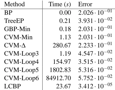
3.3 ALARM Network
The ALARM network8is a well-known Bayesian network consisting of 37 variables (some of which can take on more than two possible values) and 37 factors (many of which involve more than two variables). In addition to the usual approximate inference methods, we have compared with GBP-Min, a GBP implementation of the minimal CVM approximation that uses maximal factors as outer clusters. The results are reported in Table 1.9
The accuracy of GBP-Min (and CVM-Min) is almost identical to that of BP for this graphical model; GBP-Min converges without damping and is faster than CVM-Min. On the other hand, TreeEP significantly improves the BP result in roughly the same time as GBP-Min needs. Simply enlarging the cluster size (CVM-∆) slightly deteriorates the quality of the results and also causes an enormous increase of computation time. The quality of the CVM-Loop results is roughly compara-ble to that of TreeEP. Surprisingly, increasing the loop depth beyond 4 deteriorates the quality of the results and results in an explosion of computation time. We conclude that the CVM-Loop method is not a very good approach to correcting loops in this case. LCBP uses considerable computation time, but yields errors that are approximately 104 times smaller than BP errors. The
cumulant-8. The ALARM network can be downloaded from http://compbio.cs.huji.ac.il/Repository/Datasets/ alarm/alarm.dsc.
Method Time (s) Error BP 0.00 2.026·10−01 TreeEP 0.21 3.931·10−02 GBP-Min 0.18 2.031·10−01 CVM-Min 1.13 2.031·10−01 CVM-∆ 280.67 2.233·10−01 CVM-Loop3 1.19 4.547·10−02 CVM-Loop4 154.97 3.515·10−02 CVM-Loop5 1802.83 5.316·10−02 CVM-Loop6 84912.70 5.752·10−02 LCBP 23.67 3.412·10−05
Table 1: Results for the ALARM network
based loop LCBP methods are not available, due to the presence of factors involving more than two variables and variables that can take more than two values.
3.4 PROMEDAS Networks
In this subsection, we study the performance of LCBP on another “real world” example, the PROMEDAS medical diagnostic network (Wiegerinck et al., 1999). The diagnostic model in PROMEDAS is based on a Bayesian network. The global architecture of this network is similar to QMR-DT (Shwe et al., 1991). It consists of a diagnosis layer that is connected to a layer with findings.10 Diagnoses (diseases) are modeled as a priori independent binary variables causing a set of symptoms (findings), which constitute the bottom layer. The PROMEDAS network currently consists of approximately 2000 diagnoses and 1000 findings.
The interaction between diagnoses and findings is modeled with a noisy-OR structure. The conditional probability of the finding given the parents is modeled by m+1 numbers, m of which represent the probabilities that the finding is caused by one of the diseases and one that the finding is not caused by any of the parents.
The noisy-OR conditional probability tables with m parents can be naively stored in a table of size 2m. This is problematic for the PROMEDAS networks since findings that are affected by more than 30 diseases are not uncommon in the PROMEDAS network. We use an efficient implementa-tion of noisy-OR relaimplementa-tions as proposed by Takikawa and D’Ambrosio (1999) to reduce the size of these tables. The trick is to introduce dummy variables s and to make use of the property
OR(x|y1,y2,y3) =
∑
sOR(x|y1,s)OR(s|y2,y3).
The factors on the right hand side involve at most 3 variables instead of the initial 4 (left). Repeated application of this formula reduces all factors to triple interactions or smaller.
When a patient case is presented to PROMEDAS, a subset of the findings will be clamped and the rest will be unclamped. If our goal is to compute the marginal probabilities of the diagnostic
10−8
10−6
10−4
10−2
100
LCBP
error
LCBP
error
10−9 10−6 10−3 100
BP error BP error
10−8
10−6
10−4 10−2
100
CVM-Min
error
CVM-Min
error
10−9 10−6 10−3 100
BP error BP error
10−8 10−6 10−4
10−2 100 T reeEP error T reeEP error
10−9 10−6 10−3 100
BP error BP error
10−8
10−6
10−4
10−2 100 CVM-Lo op3 error CVM-Lo op3 error
10−9 10−6 10−3 100
BP error BP error
10−8 10−6 10−4 10−2 100 CVM-Lo op4 error CVM-Lo op4 error
10−9 10−6 10−3 100 BP error
BP error
10−8
10−6
10−4
10−2 100 CVM-Lo op5 error CVM-Lo op5 error
10−9 10−6 10−3 100
BP error BP error
Figure 13: Scatter plots of errors for PROMEDAS instances.
variables only, the unclamped findings and the diagnoses that are not related to any of the clamped findings can be summed out of the network as a preprocessing step. The clamped findings cause an effective interaction between their parents. However, the noisy-OR structure is such that when the finding is clamped to a negative value, the effective interaction factorizes over its parents. Thus, findings can be clamped to negative values without additional computation cost (Jaakkola and Jor-dan, 1999).
The complexity of the problem now depends on the set of findings that is given as input. The more findings are clamped to a positive value, the larger the remaining network of disease variables and the more complex the inference task. Especially in cases where findings share more than one common possible diagnosis, and consequently loops occur, the model can become complex.
We use the PROMEDAS model to generate virtual patient data by first clamping one of the disease variables to be positive and then clamping each finding to its positive value with probability equal to the conditional distribution of the finding, given the positive disease. The union of all positive findings thus obtained constitute one patient case. For each patient case, the corresponding truncated graphical model is generated. The number of disease nodes in this truncated graph is typically quite large.