Ranking the Best Instances
St´ephan Cl´emenc¸on CLEMENCO@ENST.FR
D´epartement TSI Signal et Images - LTCI UMR GET/CNRS 5141 Ecole Nationale Sup´erieure des T´el´ecommunications
37-39, rue Dareau 75014 Paris, France
Nicolas Vayatis VAYATIS@CMLA.ENS-CACHAN.FR
Centre de Math´ematiques et de Leurs Applications - UMR CNRS 8536 Ecole Normale Sup´erieure de Cachan - UniverSud
61, avenue du Pr´esident Wilson 94 235 Cachan cedex, France
Editor: Yoram Singer
Abstract
We formulate a local form of the bipartite ranking problem where the goal is to focus on the best instances. We propose a methodology based on the construction of real-valued scoring functions. We study empirical risk minimization of dedicated statistics which involve empirical quantiles of the scores. We first state the problem of finding the best instances which can be cast as a clas-sification problem with mass constraint. Next, we develop special performance measures for the local ranking problem which extend the Area Under an ROC Curve (AUC) criterion and describe the optimal elements of these new criteria. We also highlight the fact that the goal of ranking the best instances cannot be achieved in a stage-wise manner where first, the best instances would be tentatively identified and then a standard AUC criterion could be applied. Eventually, we state preliminary statistical results for the local ranking problem.
Keywords: ranking, ROC curve and AUC, empirical risk minimization, fast rates
1. Introduction
ranking rule (Cortes and Mohri, 2004; Freund et al., 2003; Rudin et al., 2005; Agarwal et al., 2005). In a previous work, we have mentioned that the bipartite ranking problem under the AUC crite-rion could be interpreted as a classification problem with pairs of observations (Cl ´emenc¸on et al., 2005). But the limit of this approach is that it weights uniformly the pairs of items which are badly ranked. Therefore it does not permit to distinguish between ranking rules making the same number of mistakes but in very different parts of the ROC curve. The AUC is indeed a global criterion which does not allow to concentrate on the ”best” instances. Special performance measures, such as the Discounted Cumulative Gain (DCG) criterion, have been introduced by practitioners in order to weight instances according to their rank (J¨arvelin and Kek¨al¨ainen, 2000) but providing theory for such criteria and developing empirical risk minimization strategies still is a very open issue. Recent works by Rudin (2006), Cossock and Zhang (2006), and Li et al. (2007) reveal that there are several possibilities when designing ranking algorithms with focus on the top-rated instances. In the present paper, we focus on statistical aspects rather than algorithmic. We extend the results of our previous work in Cl´emenc¸on et al. (2005) and set theoretical grounds for the problem of local ranking. The methodology we propose is based on the selection of a real-valued scoring function for which we formulate appropriate performance measures generalizing the AUC criterion. We point out that ranking the best instances is an involved task as it is a two-fold problem: (i) find the best instances and (ii) provide a good ranking on these instances. The fact that these two goals cannot be considered independently will be highlighted in the paper. Despite this observation, we will first formulate the issue of finding the best instances which is to be understood as a toy problem for our purpose. This problem corresponds to a binary classification problem with a mass constraint (where the proportion u of +1 labels predicted by the classifiers is fixed) and it might present an interest
per se. The main complication here has to do with the necessity of performing quantile estimation which affects the performance of statistical procedures. Our proof technique was inspired by the former work of Koul (2002) in the context of R-estimation where similar statistics, known as linear signed rank statistics, arise. By exploiting the structure of such statistics, we are able to establish noise conditions in a similar way as in Cl´emenc¸on et al. (To appear) where we had to deal with per-formance criteria based on U -statistics. Under such conditions, we prove that rates of convergence up to n−/ can be guaranteed for the empirical risk minimizer in the classification problem with mass constraint. Another contribution of the paper lies in our study of the optimality issue for the local ranking problem. We discuss how focusing on best instances affects the ROC curve and the AUC criterion. We propose a family of possible performance measures for the problem of ranking the best instances. In particular, we show that widespread ideas in the biostatistics literature about the partial AUC (see Dodd and Pepe, 2003) turn out to be questionable with respect to optimality considerations. We also point out that the empirical risks for local ranking are closely related to generalized Wilcoxon statistics.
2. Finding the Best Instances
In the present section, we have a limited goal which is only to determine the best instances without bothering with their order in the list. By considering this subproblem, we will identify the main technical issues involved in the sequel. It also permits to introduce the main notations of the paper.
Just as in standard binary classification, we consider the pair of random variables(X,Y)where X is an observation vector in a measurable space
X
and Y is a binary label in{−,+}. The distribution of(X,Y)can be described by the pair(µ,η)where µ is the marginal distribution of X andηis the a posteriori distribution defined by η(x) =P{Y =|X=x}, ∀x∈X
. We define the rate of best instances as the proportion of best instances to be considered and denote it by u∈(, ). Wedenote by Q(η, −u) the (−u)-quantile of the random variable η(X). Then the set of best
instances at rate uis given by:
Cu∗ ={x∈
X
|η(x)≥Q(η, −u)}.We mention two trivial properties of the set Cu∗ which will be important in the sequel:
• MASS CONSTRAINT: we have µ Cu∗=PX∈Cu∗ =u,
• INVARIANCE PROPERTY: as a functional ofη, the set Cu∗ is invariant to strictly increasing
transforms ofη.
The problem of finding a proportion u of the best instances boils down to the estimation of
the unknown set Cu∗ on the basis of empirical data. Before turning to the statistical analysis of the problem, we first relate it to binary classification.
2.1 A Classification Problem with a Mass Constraint
A classifier is a measurable function g :
X
→{−,+} and its performance is measured by the classification error L(g) =P{Y6=g(X)}. Let u∈(, ) be fixed. Denote by g∗u =ICu∗− theclassifier predicting +1 on the set of best instances C∗u and -1 on its complement. The next proposi-tion shows that g∗u is an optimal element for the problem of minimization of L(g)over the family of classifiers g satisfying the mass constraintP{g(X) =}=u.
Proposition 1 For any classifier g :
X
→{−,+}such that g(x) =IC(x) −for some subset Cof
X
and µ(C) =P{g(X) =}=u, we haveL∗u $L g∗u
≤L(g).
Furthermore, we have
L∗u=−Q(η, −u) + (−u)(Q(η, −u) −) −E(|η(X) −Q(η, −u)|),
and
L(g) −L g∗u=E |η(X) −Q(η, −u)|IC∗u
∆C(X)
,
PROOF. For simplicity, we temporarily change the notation and set q=Q(η, −u). Then, for any
classifier g satisfying the constraintP{g(X) =}=u, we have
L(g) =E (η(X) −q)I[g(X)=−]+ (q−η(X))I[g(X)=+]
+ (−u)q+ (−q)u.
The statements of the proposition immediately follow.
There are several progresses in the field of classification theory where the aim is to introduce constraints in the classification procedure or to adapt it to other problems. We relate our formulation to other approaches in the following remarks.
Remark 2 (CONNECTION TO HYPOTHESIS TESTING). The implicit asymmetry in the problem due to the emphasis on the best instances is reminiscent of the statistical theory of hypothesis testing. We can formulate a test of simple hypothesis by taking the null assumption to be H : Y = −
and the alternative assumption being H : Y = +. We want to decide which hypothesis is true
given the observation X . Each classifier g provides a test statistic g(X). The performance of the test is then described by its type I error α(g) =P{g(X) =|Y = −} and its power β(g) =
P{g(X) =|Y = +}. We point out that if the classifier g satisfies a mass constraint, then we can relate the classification error with the type I error of the test defined by g through the relation:
L(g) =(−p)α(g) +p−u
where p=P{Y =}, and similarly, we have: L(g) =p(−β(g)) −p−u. Therefore, the optimal
classifier minimizes the type I error (maximizes the power) among all classifiers with the same mass constraint. In some applications, it is more relevant to fix a constraint on the probability of a false alarm (type I error) and maximize the power. This question is explored in a recent paper by Scott (2005) (see also Scott and Nowak, 2005).
Remark 3 (CONNECTION WITH REGRESSION LEVEL SET ESTIMATION) We mention that the es-timation of the level sets of the regression function has been studied in the statistics literature (Cav-alier, 1997) (see also Tsybakov, 1997 and Willett and Nowak, 2006) as well as in the learning literature, for instance in the context of anomaly detection (Steinwart et al., 2005; Scott and Daven-port, 2006, to appear; Vert and Vert, 2006). In our framework of classification with mass constraint, the threshold defining the level set involves the quantile of the random variableη(X).
Remark 4 (CONNECTION WITH THE MINIMUM VOLUME SET APPROACH) Although the point of
view adopted in this paper is very different, the problem described above may be formulated in the framework of minimum volume sets learning as considered in Scott and Nowak (2006). As a matter of fact, the set C∗u may be viewed as the solution of the constrained optimization problem:
min
C P{X∈C|Y = −}
over the class of measurable sets C, subject to
P{X∈C}≥u.
measure. We believe that learning methods for minimum volume set estimation may hopefully be extended to our setting. A natural way to do it would consist in replacing conditional distribution of X given Y = −by its empirical counterpart. This is beyond the scope of the present paper but will be the subject of future investigation.
2.2 Empirical Risk Minimization
We now investigate the estimation of the set Cu∗ of best instances at rate ubased on training data.
Suppose that we are given n i.i.d. copies(X,Y),···,(Xn,Yn)of the pair(X,Y). Since we have the
ranking problem in mind, our methodology will consist in building the candidate sets from a class
S
of real-valued scoring functions s :X
→R. Indeed, we consider sets of the formCs$Cs,u ={x∈
X
|s(x)≥Q(s, −u)},where s is an element of
S
and Q(s, −u) is the(−u)-quantile of the random variable s(X).Note that such sets satisfy the same properties of Cu∗ with respect to mass constraint and invariance to strictly increasing transforms of s.
From now on, we will take the simplified notation:
L(s)$L(s,u)$L(Cs) =P{Y·(s(X) −Q(s, −u))< } .
A scoring function minimizing the quantity
Ln(s) =
n
n X
i=
I{Yi·(s(Xi) −Q(s, −u))< }.
is expected to approximately minimize the true error L(s), but the quantile depends on the unknown distribution of X . In practice, one has to replace Q(s, −u)by its empirical counterpartQ^(s, −u)
which corresponds to the empirical quantile. We will thus consider, instead of Ln(s), the empirical
error:
^ Ln(s) =
n
n X
i=
I{Yi·(s(Xi) − ^Q(s, −u))< }.
Note that L^n(s) is a complicated statistic since the empirical quantile involves all the instances
X, . . . ,Xn. We also mention that ^Ln(s) is a biased estimate of the classification error L(s)of the
classifier gs(x) =I{s(x)≥Q(s, −u)}−.
We introduce some more notations. Set, for all t ∈R:
• Fs(t) =P{s(X)≤t}
• Gs(t) =P{s(X)≤t|Y = +}
• Hs(t) =P{s(X)≤t|Y = −}.
The functions Fs (respectively Gs, Hs) denote the cumulative distribution function (cdf) of s(X)
(respectively, given Y =, given Y = −). We recall that the definition of the quantiles of (the distribution of) a random variable involves the notion of generalized inverse F−of a function F:
Thus, we have, for all v∈(, ):
Q(s,v) =Fs−(v) and Q^(s,v) = ^Fs−(v)
whereF^sis the empirical cdf of s(X):F^s(t) = nPni=I{s(Xi)≤t},∀t∈R.
Without loss of generality, we will assume that all scoring functions in
S
take their values in (,λ)for someλ> . We now turn to study the performance of minimizers ofL^n(s)over a classS
of scoring functions defined by
^
sn=arg min s∈S
^ Ln(s).
Our first main result is an excess risk bound for the empirical risk minimizer ^snover a class
S
of uniformly bounded scoring functions. In the following theorem, we consider that the level sets of scoring functions from the class
S
form a Vapnik-Chervonenkis (VC) class of sets.Theorem 5 We assume that
(i) the class
S
is symmetric (that is, if s∈S
thenλ−s∈S
) and is a VC major class of functions with VC dimension V .(ii) the family
K
={Gs,Hs : s∈S
}of cdfs satisfies the following property: any K∈K
has leftand right derivatives, denoted by K+0 and K−0, and there exist strictly positive constants b, B
such that∀(K,t)∈
K
×(,λ),b≤K+0(t)
≤B and b≤ K−0(t)
≤B.
For anyδ> , we have, with probability larger than−δ,
L(^sn) −inf
s∈SL(s)≤c
r
V n +c
r
ln(/δ)
n ,
for some positive constants c,c.
The following remarks provide some insights on conditions (i) and (ii) of the theorem.
Remark 6 (ON THE COMPLEXITY ASSUMPTION) On the terminology of major sets and major classes, we refer to Dudley (1999). In the proof, we need to control empirical processes indexed by sets of the form{x : s(x)≥t}or{x : s(x)≤t}. Condition (i) guarantees that these sets form a VC class of sets.
Remark 7 (ON THE CHOICE OF THE CLASS
S
OF SCORING FUNCTIONS) In order to grasp the meaning of condition (ii) of the theorem, we consider the one-dimensional case with real-valued scoring functions. Assume that the distribution of the random variable Xihas a bounded density fwith respect to Lebesgue measure. Assume also that scoring functions s are differentiable except, possibly, at a finite number of points, and derivatives are denoted by s0. Denote by fsthe density of
s(X). Let t∈(,λ)and denote by x, ..., xp the real roots of the equation s(x) =t. We can express
the density of s(X)thanks to the change-of-variable formula (see, for instance, Papoulis, 1965):
fs(t) =
f(x)
s0(x)+. . .+
f(xp)
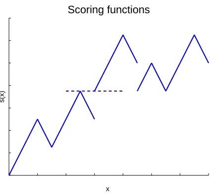
Scoring functions
x
s(x)
Figure 1: Typical example of a scoring function.
This shows that the scoring functions should not present neither flat nor steep parts. We can take for instance, the class
S
to be the class of linear-by-parts functions with a finite number of local extrema and with uniformly bounded left and right derivatives:∀s∈S
,∀x, m≤s+0 (x)≤M and m≤ s−0(x)≤M for some strictly positive constants m, and M (see Figure 1). Note that any subintervalof[,λ] has to be in the range of scoring functions s (if not, some elements of
K
will present a plateau). In fact, the proof requires such a behavior only in the vicinity of the points corresponding to the quantiles Q(s, −u)for all s∈S
.PROOF. Set v=−u. By a standard argument (see, for instance, Devroye et al., 1996), we have:
L(^sn) −inf
s∈SL(s)≤sups∈S
L^n(s) −L(s)
≤sup
s∈S
L^n(s) −Ln(s)
+sup
s∈S
|Ln(s) −L(s)| .
Note that the second term in the bound is an empirical process whose behavior is well-known. In our case, assumption (i) implies that the class of sets {x :s(x)≥Q(s,v)} indexed by scoring
functions s has a VC dimension smaller than V . Hence, we have by a concentration argument combined with a VC bound for the expectation of the supremum (see, for instance, Lugosi), for any δ> , with probability larger than−δ,
sup
s∈S
|Ln(s) −L(s)|≤c
r
V n +c
0
r
ln(/δ) n
for universal constants c,c0.
The novel part of the analysis lies in the control of the first term and we now show how to handle it. Following the work of Koul (2002), we set the following notations:
M(s,v) =PY· s(X) −Q(s,v)
Un(s,v) = n n X i=
I{Yi· s(Xi) −Q(s,v)
< }−M(s,v).
and note that Un(s,v)is centered. In particular, we have:
Ln(s) =Un(s,v) +M(s,v).
As Q(s,v) =Fs−(v), we have Q(s,Fs◦F^s−(v)) = ^Fs−(v) = ^Q(s,v)and then
^
Ln(s) =Un(s,Fs◦F^s−(v)) +M(s,Fs◦F^s−(v)).
Note that M(s,Fs◦F^s−(v)) =PY· s(X) − ^Q(s,v)< |Dn where Dndenotes the sample(X,Y),···,(Xn,Yn).
We then have the following decomposition, for any s∈
S
and v∈(, ):
^Ln(s) −Ln(s) ≤
Un(s,Fs◦F^s−(v)) −Un(s,v) +
M(s,Fs◦F^s−(v)) −M(s,v) .
Recall the notation p=P{Y =}. Since M(s,v) = (−p)(−Hs◦Fs−(v)) +pGs◦Fs−(v)and
Fs=pGs+ (−p)Hs, the mapping v7→M(s,v)is Lipschitz by assumption (ii). Thus, there exists a constantκ<∞, depending only on p, b and B, such that:
M(s,Fs◦F^s−(v)) −M(s,v) ≤κ
Fs◦F^s−(v) −v .
Moreover, we have, for any s∈
S
:
Fs◦F^s−(v) −v ≤
Fs◦F^s−(v) − ^Fs◦F^s−(v) +
F^s◦F^s−(v) −v
≤ sup
t∈(,λ)
Fs(t) − ^Fs(t) +
n .
Here again, we can use assumption (i) and a classical VC bound from Lugosi in order to control the empirical process, with probability larger than−δ:
sup
(s,t)∈S×(,λ)
Fs(t) − ^Fs(t) ≤c
r
V n +c
0
r
ln(/δ) n
for some constants c,c0.
It remains to control the term involving the process Un:
Un(s,Fs◦F^s−(v)) −Un(s,v)
≤ sup
v∈(,)
|Un(s,v) −Un(s,v)|≤ sup v∈(,)
|Un(s,v)|.
Using that the class of sets of the form{x:s(x)≥Q(s,v)}for v∈(, )is included in the class of sets of the form{x :s(x)≥t}where t∈(,λ), we then have
sup
v∈(,)
|Un(s,v)|≤ sup
t∈(,λ) n n X i=
I{Yi· s(Xi) −t
< }−PY· s(X) −t
< ,
2.3 Fast Rates of Convergence
We now propose to examine conditions leading to fast rates of convergence (faster than n−/). It has been noticed (see Mammen and Tsybakov, 1999; Tsybakov, 2004; Massart and N ´ed´elec, 2006) that it is possible to derive such rates of convergence in the classification setup under additional assumptions on the distribution. We propose here to adapt these assumptions for the problem of classification with mass constraint.
Our concern here is to formulate the type of conditions which render the problem easier from a statistical perspective. For this reason and to avoid technical issues, we will consider a quite restrictive setup where it is assumed that:
• the class
S
of scoring functions is a finite class with N elements,• an optimal scoring rule s∗is contained in
S
.We have found that the following additional conditions on the distribution and the class
S
allow to derive fast rates of convergence for the excess risk in our problem.(iii) There exist constantsα∈(, )and D> such that, for all t ≥,
P{|η(X) −Q(η, −u)|≤t}≤Dt
α
−α .
(iv) the family
K
={Gs,Hs : s∈S
}of cdfs satisfies the following property: for any s∈S
, Gsand Hsare twice differentiable at Q(s, −u) =Fs−(−u).
Note that condition (iii) simply extends the standard low noise assumption introduced by Tsy-bakov (2004) (see also Boucheron et al., 2005, for an account on this) where the level 1/2 is replaced by the(−u)-quantile ofη(X). Condition (iv) is a technical requirement needed in order to derive
an approximation of the statistics involved in empirical risk minimization.
Remark 8 (CONSEQUENCE OF CONDITION (III)) We recall here the various equivalent formula-tions of condition (iii) as they are described in Section 5.2 from the survey paper by Boucheron et al. (2005). A slight variation in our setup is due to the presence of the quantile Q(η, −u) but we
can easily adapt the corresponding conditions. Hence, we have, under condition (iii), the variance control, for any s∈
S
:Var(I{Y 6=ICs(X) −}−I{Y 6=ICu∗(X) −})≤c(L(s) −L
∗
u)
α,
or, equivalently,
E ICs∆Cu∗(X)
≤c(L(s) −L∗u)α.
Recall that Ln(s) =nPin=I{Yi·(s(Xi) −Q(s, −u))< }. We point out that Ln(s)is not an
empiri-cal criterion since the quantile Q(s, −u)depends on the distribution. However, we can introduce
the minimizer of this functional:
sn=arg min s∈S
Ln(s),
for which we can use the same argument as in the classification setup. We then have, by a standard argument based on Bernstein’s inequality (which will be provided for completeness in the proof of Theorem 10 below), with probability−δ,
L(sn) −L∗u ≤c
log(N/δ) n
−α
for some positive constant c. We will show below how to obtain a similar rate when the true quantile Q(s, −u)is replaced by the empirical quantileQ^(s, −u)in the criterion to be minimized.
We point out that conditions (ii) and (iii) are not completely independent. We offer the following proposition which will be useful in the sequel.
Proposition 9 If(Gη,Hη)belongs to the class
K
fulfilling condition (ii), then Fη is Lipschitz and condition (iii) is satisfied withα=/.PROOF. We recall that Fη = pGη+ (−p)Hη and assume for simplicity that Gη and Hη are
differentiable. By condition (ii), we then have|F0
η|= p|Gη0|+ (−p)|Hη0|≤pB+ (−p)B=B.
Set q=Q(η, −u). Then, by the mean value theorem, there exists a constant c such that, for all
t≥:
P{|η(X) −q|≤t}=Fη(t+q) −Fη(−t+q)≤B(t+q− (−t+q)) =Bt .
We have proved that condition (iii) is fulfilled with D=B andα=/.
The novel part of the analysis below lies in the control of the bias induced by plugging the empirical quantileQ^(s, −u) in the risk functional. The next theorem shows that faster rates of
convergence up to the order of n−/can be obtained under the previous assumptions.
Theorem 10 We assume that the class
S
of scoring functions is a finite class with N elements, and that it contains an optimal scoring rule s∗. Moreover, we assume that conditions (i)-(iv) are satisfied. We recall thats^n=arg mins∈SL^n(s). Then, for anyδ> , we have, with probability−δ:L(^sn) −L∗u ≤c
log(N/δ) n
,
for some constant c.
Remark 11 (ON THE RATEn−/) This result highlights the fact that rates faster than the one
ob-tained in Theorem 5 can be obob-tained in this setup with additional regularity assumptions. However, it is noteworthy that the standard low noise assumption (iii) is already contained, by Proposition 9, in assumption (ii) which is required in proving the typical n−/ rate. The consequence of this observation is that there is no hope of getting rates up to n−unless assumption (ii) is weakened.
Remark 12 (ON THE ASSUMPTIONs∗∈
S
) This assumption is not important and can be removed. For a neat argument, check the proof of Theorem 5 from Cl´emenc¸on et al. (To appear) which uses a result by Massart (2006).The proof of the previous theorem is based on two arguments: the structure of linear signed rank statistics and the variance control assumption. The situation is similar to the one we encountered in Cl´emenc¸on et al. (To appear) where we were dealing with U-statistics and we had to invoke Hoeffding’s decomposition in order to grasp the behavior of the underlying U-processes. Here we require a similar argument to describe the structure of the empirical risk functional ^Ln(s) under
refer to H´ajek and Sid´ak (1967), Dupac and H´ajek (1969), Koul (1970), and Koul and R.G. Staudte (1972) for an account on rank statistics.
We now prepare for the proof by stating the main ideas in the next propositions, but first we need to introduce some notations. Set:
∀v∈[, ], K(s,v) =E(YI{s(X)≤Q(s,v)}) =pGs(Q(s,v)) − (−p)Hs(Q(s,v)),
^
Kn(s,v) =
n
n X
i=
YiI{s(Xi)≤Q^(s,v)}.
Then we can write:
L(s) =−p+K(s, −u),
^ Ln(s) =
n−
n + ^Kn(s, −u),
where n−=Pni=I{Yi= −}.
We note that the statistic^Ln(s)is related to linear signed rank statistics.
Definition 13 (Linear signed rank statistic) Consider Z, . . . ,Znan i.i.d. sample with distribution
F and a real-valued score generating functionΦ. Denote by R+i =rank(|Zi|)the rank of|Zi|in the
sample|Z|, . . . ,|Zn|. Then the statistic
n X
i=
Φ R+i
n+
sgn(Zi)
is a linear signed rank statistic.
Proposition 14 For fixed s and v, the statisticK^n(s,v)is a linear signed rank statistic.
PROOF. Take Zi=Yis(Xi). The random variables Zi have their absolute value distributed according
to Fsand have the same sign as Yi. It is easy to see that the statisticK^n(s,v)is a linear signed rank
statistic with score generating functionΦ(x) =I[x≤v].
A decomposition of Hoeffding’s type for such statistics can be formulated. Set first:
Zn(s,v) =
n
n X
i=
Yi−K0(s,v)
I{s(Xi)≤Q(s,v)}−K(s,v) +vK0(s,v),
where K0(s,v)denotes the derivative of the function v7→K(s,v). Note that Zn(s,v) is a centered
random variable with variance:
σ(s,v) =v−K(s,v)+v(−v)K0(s,v) −(−v)K0(s,v)K(s,v).
Proposition 15 Assume that condition (iv) holds. We have, for all s∈
S
and v∈[, ]:^
Kn(s,v) =K(s,v) +Zn(s,v) +Λn(s).
with
Λn(s) =OP(n−) as n→ ∞.
This asymptotic expansion highlights the structure of the statistic^Ln(s)for fixed s:
^ Ln(s) =
n−
n +K(s, −u) +Zn(s, −u) +Λn(s).
Once centered, the leading term Zn(s, −u)is an empirical average of i.i.d. random variables (of a
stochastic order of n−/) and the remainder termΛn(s)is of a stochastic order of n−. The nature of
the decomposition of^Ln(s)is certainly unexpected because the leading term contains an additional
derivative term given by K0(s, −u) (v−I{s(Xi)≤Q(s, −u)}). The revelation of this fact is one
of the major contributions in the work of Koul (2002).
Now, in order to establish consistency and rates-of-convergence-type results, we need to fo-cus only on the leading term which carries most of the statistical information, while the remainder needs to be controlled uniformly over the candidate class
S
. As a consequence, the variance con-trol assumption will only concern the variance of the kernel hs involved in the empirical averageZn(s, −u)and defined as follows:
hs(Xi,Yi) = Yi−K0(s,v)
I{s(Xi)≤Q(s,v)}−K(s,v) +vK0(s,v),
We then have
Zn(s,v) −Zn(s∗,v) =
n
n X
i=
hs(Xi,Yi) −hs∗(Xi,Yi).
Proposition 16 Fix v∈[, ]. Assume that condition (iii) holds. Then, we have, for all s∈
S
:Var hs(Xi,Yi) −hs∗(Xi,Yi)
≤c L(s) −L(s∗)α
,
for some constant c.
PROOF. We first write that:
hs(Xi,Yi) −hs∗(Xi,Yi) =I+II+III+IV+V
where
I = Yi I{s(Xi)≤Q(s,v)}−I{s∗(Xi)≤Q(s∗,v)}
,
II = (K0(s∗,v) −K0(s,v))I{s∗(X
i)≤Q(s∗,v)},
III = K0(s,v) I{s∗(Xi)≤Q(s∗,v)}−I{s(Xi)≤Q(s,v)}
,
IV = K(s∗,v) −K(s,v),
By Cauchy-Schwarz inequality, we only need to show that the expected value of the square of these quantities is smaller than(L(s) −L∗)αup to some multiplicative constant.
Note that, by definition of K, we have:
II = (L0(s∗,v) −L0(s,v))I{s∗(Xi)≤Q(s∗,v)},
IV = L(s∗) −L(s),
V = v(L0(s,v) −L0(s∗,v))
where L0(s,v) denotes the derivative of the function v7→L(s,v). It is clear that, for any s, we have L(s,v) =L(s∗,v)implies that L0(s,v) =L0(s∗,v)otherwise s∗would not be an optimal scoring function at some level v0 in the vicinity of v. Therefore, since
S
is finite, there exists a constant c such that(L0(s,v) −L0(s∗,v))≤c(L(s) −L∗)α
and thenE II
andE V
are bounded accordingly. Moreover, we have:
E I≤E ICs∆Cs∗(X)
≤c(L(s) −L(s∗))α
for some positive constant c, by assumption (iii).
Eventually, by assumption (ii), we have that K0(s,v)is uniformly bounded and thus, the term
E IIIcan be handled similarly.
Proof of Theorem 10. Set v=−u. First notice thats^n=arg mins∈SK^n(s, −u). We then have
L(^sn) −L(s∗) =K(^sn,v) −K(s∗,v)
≤K^n(s∗,v) − ^Kn(^sn,v) − (K(s∗,v) −K(^sn,v))
≤Zn(s∗,v) −Zn(^sn,v)) +sup s∈S
|Λn(s)|
where we used the decomposition of the linear signed rank statistic from Proposition 15 to obtain the last inequality.
By Proposition 15, we know that the second term on the right hand side is of stochastic order n− since the class
S
is of finite cardinality. It remains to control the leading term Zn(s∗,v) −Zn(^sn,v).At this point, we will use the same argument as in Section 5.2 from Boucheron et al. (2005). Denote by C=sups,x,y|hs(x,y)|and byσ(s) =Var hs(Xi,Yi) −hs∗(Xi,Yi). By Bernstein’s in-equality for averages of upper bounded and centered random variables (see Devroye et al., 1996) and the union bound, we have, with probability−δ, for all s∈
S
:Zn(s∗,v) −Zn(s,v)≤ r
σ(s)log(N/δ)
n +
≤ r
c(L(s) −L∗)α log(N/δ)
n +
C log(N/δ) n
thanks to the variance control obtained in Proposition 16. Since this inequality holds for any s, it holds in particular for s= ^sn. Therefore, we have obtained the following result, with probability −δ:
L(^sn) −L(s∗)≤
r
c(L(^sn) −L∗)α log(N/δ)
n +
c0log(N/δ) n
for some constants c, c0. At the cost of increasing the multiplicative constant factor, we can get rid of the second term and solve the inequality in the quantity L(^sn) −L(s∗)to get
L(^sn) −L(s∗)≤c
log(N/δ) n
−α
for some constant c. To end the proof, we plug the value ofα=/following from Proposition 9.
3. Performance Measures for Local Ranking
Our main interest here is to develop a setup describing the problem of not only finding but also ranking the best instances. In the sequel, we build on the results from Section 2 and also on our previous work on the (global) ranking problem (Cl´emenc¸on et al., To appear) in order to capture some of the features of the local ranking problem. The present section is devoted to the construction of performance measures reflecting the quality of ranking rules on a restricted set of instances.
3.1 ROC Curves and Optimality in the Local Ranking Problem
We consider the same statistical model as before with(X,Y)being a pair of random variables over
X
×{−,+}and we examine ranking rules resulting from real-valued scoring functions s :X
→ (,λ). The reference tool for assessing the performance of a scoring function s in separating the two populations (positive vs. negative labels) is the Receiver Operating Characteristic known as the ROC curve (van Trees, 1968; Egan, 1975). If we take the notations ¯Gs(z) =P{s(X)>z | Y=}(true positive rate) and ¯Hs(z) =P{s(X)>z | Y= −}(false positive rate), we can define the ROC
curve, for any scoring function s, as the plot of the function:
z7→ H¯s(z),G¯s(z)
for thresholds z∈(,λ), or equivalently as the plot of the function:
t7→G¯s◦Hs−(−t)
curve of any other scoring function. We point out that the ROC curve of a scoring function s is invariant to strictly increasing transformations of s.
In our approach, for a given scoring function s, we focus on thresholds z corresponding to the cut-off separating a proportion u∈(, )of top scored instances according to s from the rest. Recall from Section 2 that the best instances according to s are the elements of the set Cs,u={x∈
X
|s(x)≥Q(s, −u)}where Q(s, −u)is the(−u)-quantile of s(X). We set the following notations:
α(s,u) =P{s(X)≥Q(s, −u)|Y= −}=H¯s◦Fs−(−u),
β(s,u) =P{s(X)≥Q(s, −u)|Y = +}=G¯s◦F−
s (−u).
We propose to re-parameterize the ROC curve with the proportion u∈(, )and then describe it as the plot of the function:
u7→(α(s,u),β(s,u)),
for each scoring function s. When focusing on the best instances at rate u, we only consider the
part of the ROC curve for values u∈(,u).
However attractive is the ROC curve as a graphical tool, it is not a practical one for developing learning procedures achieving straightforward optimization. The most natural approach is to con-sider risk functionals built after the ROC curve such as the Area Under an ROC Curve (known as the AUC or AROC, see Hanley and McNeil, 1982). Our goals in this section are:
1. to extend the AUC criterion in order to focus on restricted parts of the ROC curve,
2. to describe the optimal elements with respect to this extended criterion.
We point out the fact that extending the AUC is not trivial. In order to focus on the best instances, a natural idea is to truncate the AUC (as in the approach by Dodd and Pepe (2003)).
Definition 17 (Partial AUC) We define the partial AUC for a scoring function s and a rate u of best instances as:
PARTAUC(s,u) =
Zα(s,u)
β(s,α)dα.
We conjecture that such a criterion is not appropriate for local ranking. If it was, then we should have: ∀s,PARTAUC(s,u)≤PARTAUC(η,u), since the function η would provide the optimal
ranking. However, there is strong evidence that this is not true as shown by a simple geometric argument which we describe below.
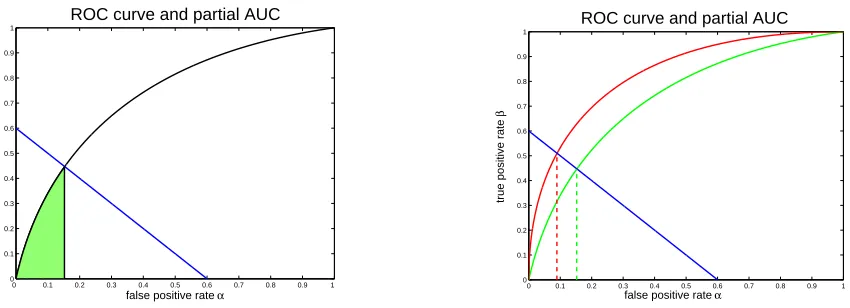
In order to represent the partial AUC of a scoring function s, we need to locate the cut-off point given the constraint on the rate uof best instances. We notice thatα(s,u)andβ(s,u)are related by
a linear relation, for fixed u and p, when s varies:
u=pβ(s,u) + (−p)α(s,u)
where p=P{Y =}. We denote the line plot of this relation by D(u,p)and call it the control line when u=u. Hence, the part of the ROC curve of a scoring function s corresponding to the best
instances at rate u is the part going from the origin(, )to the intersection with the control line
D(u,p). The partial AUC is then the area under this part of the ROC curve (it corresponds to the
0 0.1 0.2 0.3 0.4 0.5 0.6 0.7 0.8 0.9 1 0
0.1 0.2 0.3 0.4 0.5 0.6 0.7 0.8 0.9 1
ROC curve and partial AUC
false positive rate α
true positive rate
β
0 0.1 0.2 0.3 0.4 0.5 0.6 0.7 0.8 0.9 1
0 0.1 0.2 0.3 0.4 0.5 0.6 0.7 0.8 0.9 1
ROC curve and partial AUC
true positive rate
β
false positive rate α
Figure 2: ROC curves, control line D(u,p)and partial AUC at rate uof best instances.
The optimality ofηwith respect to the partial AUC can then be questioned. Indeed, the closer to ηthe scoring function s is, the higher the ROC curve is, but at the same time the integration domain shrinks (right display of Figure 2) so that the overall impact on the integral is not clear. Let us now put things formally in the following lemma.
Lemma 18 For any scoring function s, we have for all u∈(, ),
β(s,u)≤β(η,u),
α(s,u)≥α(η,u).
Moreover, we have equality only for those s such that Cs,u=Cu∗.
PROOF. We show the first inequality. By definition, we have:
β(s,u) =−Gs(Q(s, −u)).
Observe that, for any scoring function s,
p(−Gs(Q(s, −u)) =P{Y=,s(X)>Q(s, −u)} =E(η(X)I{X∈Cs,u}) .
We thus have
p(Gs(Q(s, −u) −Gη(Q(η, −u)) =E(η(X)(I{X∈Cu∗}−I{X ∈Cs,u}))
=E(η(X)I{X ∈/Cu∗}(I{X∈C∗u}−I{X∈Cs,u}))
+E(η(X)I{X ∈Cu∗}(I{X ∈Cu∗}−I{X∈Cs,u}))
≥−E(Q(η, −u)I{X∈/Cu∗}I{X∈Cs,u})
=Q(η, −u)(−u−+u) = .
The second inequality simply follows from the identity below:
−u=pGs(Q(s, −u)) + (−p)Hs(Q(s, −u)).
The previous lemma will be important when describing the optimal rules for local ranking cri-teria. But, at this point, we still do not know any nice criterion for the problem of ranking the best instances. Before considering different heuristics for extending the AUC criterion in the next subsections, we will proceed backwards and define our target, that is to say, the optimal scoring functions for our problem.
Definition 19 (Class
S
∗of optimal scoring functions) The optimal scoring functions for rankingthe best instances at the rate u are defined as the members of the equivalence class (functions
defined up to the composition with a nondecreasing transformation) of scoring functions s∗ such that:
s∗(x) =
η(x) if x∈Cu∗
< inf
z∈C∗
u
η(z) if x∈/Cu∗ .
Such scoring functions fulfill the two properties of locating the best instances (indeed Cs∗,u = C∗u) and ranking them as well as the regression function.
Under the light of Lemma 18, we will see that a wide collection of criteria with the set
S
∗as the set of optimal elements could naturally be considered, depending on how one wants to weight the two types of error−β(s,u)(type II error in the hypothesis testing framework) andα(s,u)(type I error) according to the rate u∈[,u]. However, not all the criteria obtained in this manner can beinterpreted as generalizations of the AUC criterion for u=.
3.2 Generalization of the AUC Criterion
In Cl´emenc¸on et al. (To appear), we have considered the ranking error of a scoring function s as defined by:
R(s) =P{(Y−Y0)(s(X) −s(X0))< },
where(X0,Y0)is an i.i.d. copy of the random pair(X,Y).
Interestingly, it can be proved that minimizing the ranking error R(s)is equivalent to maximizing the well-known AUC criterion. This is trivial once we write down the probabilistic interpretation of the AUC:
AUC(s) =Ps(X)>s(X0)|Y=,Y0= − =−
p(−p)R(s).
We now propose a local version of the ranking error on a measurable set C⊂
X
:On sets of the form C=Cs,u={x∈
X
|s(x)≥Q(s, −u)}with mass equal to u, the local rankingerror will be denoted by R(s,u)$R(s,Cs,u).
We will also consider the local analogue of the AUC criterion:
LOCAUC(s,u) =Ps(X)>s(X0), s(X)≥Q(s, −u) | Y =,Y0= − .
This criterion obviously boils down to the standard criterion for u=. However, in the case where u< , we will see that there is no equivalence between maximizing the LOCAUC criterion and minimizing the local ranking error s7→R(s,u). Indeed, the local ranking error is not a relevant performance measure for finding the best instances. Minimizing it would solve the problem of finding the instances that are the easiest to rank.
The following theorem states that optimal scoring functions s∗in the set
S
∗maximize the LO-CAUC criterion and that the latter may be decomposed as a sum of a ’power’ term and (the opposite of) a local ranking error term.
Theorem 20 Let u∈(, ). We have, for any scoring function s:
∀s∗∈
S
∗, LOCAUC(s,u)≤LOCAUC(s∗,u).Moreover, the following relation holds:
∀s, LOCAUC(s,u) =β(s,u) −
p(−p)R(s,u),
where R(s,u) =R(s,Cs,u).
PROOF. We first introduce the notation for the Lebesgue-Stieltjes integral. Wheneverϕis a cdf on
Randψis integrable, the integralRψ(z)dϕ(z)denotes the Lebesgue-Stieltjes integral (integration with respect to the measureνdefined by ν[a,b) =ϕ(b) −ϕ(a)for any real numbers a<b). Ifϕ has a density with respect to the Lebesgue measure, then the integral can be written as a Lebesgue integral: Rψ(z)dϕ(z) =Rψ(z)ϕ0(z)dz. We shall use this convention repeatedly in the sequel. In particular, if Z is a random variable with cdf given by FZ then we can write: E(Z) =
R
z dFZ(z).
Now set v=−u. Observe first that, by conditioning on X , we have:
LOCAUC(s,u) =E I{s(X)>s(X0)}I{s(X)≥Q(s,v)} |Y =,Y0= −
=E I{s(X)≥Q(s,v)}E I{s(X)>s(X0)} |Y0= −,X |Y =
=E(Hs(s(X))I{s(X)≥Q(s,v)} |Y=)
= Z+∞
Q(s,v)
Hs(z)dGs(z).
The last equality is obtained by using the fact that, conditionally on Y=, the random variable s(X) has cdf Gs. We now use that pGs=Fs− (−p)Hsand we obtain:
pLOCAUC(s,u) =
Z+∞
Q(s,v)
Hs(z)dFs(z) − (−p) Z+∞
Q(s,v)
Recall now thatα(s,v) =H¯s◦Fs−(−v)and make the change of variable−v=Fs(z)
Z+∞
Q(s,v)
Hs(z)dFs(z) = Zv
(−α(s,v))dv.
The second term is computed by making the change of variable a=Hs(z)which leads to:
Z+∞
Q(s,v)
Hs(z)dHs(z) = Z
−α(s,u)
a da.
We have obtained:
pLOCAUC(s,u) =
Zv
(−α(s,v))dv−−p
(− (−α(s,v)) ) .
From Lemma 18, we have that, for any u∈(, ), the functional s7→α(s,u))is minimized for s=η. Hence, the first part of Theorem 20 is established.
Besides, integrating by parts, we get:
Z+∞
Q(s,v)
Hs(z)dGs(z) = [Hs(z)Gs(z)]+Q∞(s,v)−
Z+∞
Q(s,v)
Gs(z)dHs(z).
The same change of variables as before leads to:
Z+∞
Q(s,v)
Gs(z)dHs(z) = Zα(s,u)
(−β(s,α))dα.
We then have another expression of the LOCAUC(s,u):
LOCAUC(s,u) =
Zα(s,u)
β(s,α)dα+β(s,u)(−α(s,u)).
We develop further by expressing the product of α andβ in terms of probability. Using the independence of(X,Y)and(X0,Y0), we obtain:
α(s,u)β(s,u) =
p(−p)P
s(X)∧s(X0)>Q(s,v),Y =,Y0= −
=Ps(X)>s(X0),s(X)∧s(X)>Q(s,v) | Y =,Y0= −
+
p(−p)P
s(X)<s(X0),(X,X0)∈Cs,u,Y =,Y0= −
= Zα(s,u)
β(s,α)dα+
p(−p)R(s,u).
Remark 21 (TRUNCATING THEAUC) In the theorem, we obviously recover the relation between the standard AUC criterion and the (global) ranking error when u=. Besides, by checking the
proof, one may relate the generalized AUC criterion to the partial AUC. As a matter of fact, we have:
∀s, LOCAUC(s,u) =PARTAUC(s,u) +β(s,u) −α(s,u)β(s,u).
The valuesα(s,u)andβ(s,u)are the coordinates of the intersecting point between the ROC curve
of the scoring function s and the control line D(u,p). The theorem reveals that evaluating the local
performance of a scoring statistic s(X)by the truncated AUC as proposed in Dodd and Pepe (2003) is highly arguable since the maximizer of the functional s7→PARTAUC(s,u)is usually not in
S
∗.3.3 Generalized Wilcoxon Statistic
We now propose a different extension of the plain AUC criterion. Consider(X,Y),. . .,(Xn,Yn), n
i.i.d. copies of the random pair(X,Y). The intuition relies on a well-known relationship between Mann-Whitney and Wilcoxon statistics. Indeed, a natural empirical estimate of the AUC is the rate of concording pairs:
[
AUC(s) = n+n−
X
≤i,j≤n
I{Yi= −,Yj=,s(Xi)<s(Xj)},
with n+=n−n−=Pni=I{Yi= +}.
It will be useful to have in mind the definition of a linear rank statistic.
Definition 22 (linear rank statistic) Consider Z, . . . ,Zn an i.i.d. sample with distribution F and
a real-valued score generating function Φ. Denote by Ri =rank(Zi) the rank of Zi in the sample
Z, . . . ,Zn. Then the statistic
n X
i=
ciΦ
Ri
n+
is a linear rank statistic.
We refer to H´ajek and Sid´ak (1967) and van de Vaart (1998) for basic results related to linear rank statistics. In particular, we recall that, for fixed s, the Wilcoxon statistic Tn(s) is a linear
rank statistic for the sample s(X), . . . ,s(Xn), with random weights ci=I{Yi=}, score generating
functionΦ(v) =v:
Tn(s) = n X
i=
I{Yi=}
rank(s(Xi))
n+ ,
where rank(s(Xi))denotes the rank of s(Xi)in the sample{s(Xj), ≤j≤n}. The following relation
is well-known:
n+n−
n+AUC[(s) +
n+(n++)
=Tn(s).
Moreover, the statistic Tn(s)/n+is an asymptotically normal estimate of
W(s) =E(Fs(s(X))|Y =) .
Note the theoretical counterpart of the previous relation may be written as
Now, in order to take into account a proportion u of the highest ranks only, we introduce the
following quantity:
Definition 23 (W-ranking performance measure) Consider the criterion related to the score
gen-erating functionΦu(v) =vI{v> −u}:
W(s,u) =E(Φu(Fs(s(X)))|Y =).
It will be called the W -ranking performance measure at rate u.
Note that the empirical counterpart of W(s,u)is given by Tn(s,u)/n+, with
Tn(s,u) = n X
i=
I{Yi=}Φu
rank(s(Xi))
n+
.
Using the results from the previous subsection, we can easily check that the following theorem holds.
Theorem 24 We have, for all s:
∀s∗∈
S
∗, W(s,u)≤W(s∗,u).Furthermore, we have:
W(s,u) = p
β(s,u)(−β(s,u)) + (−p)LOCAUC(s,u).
PROOF. We start by the definition of W :
W(s,u) =E(Fs(s(X))I{Fs(s(X))> −u} |Y =)
= Z+∞
Q(s,−u)
Fs(z)dGs(z).
We recall that: Fs= pGs+ (−p)Hswhich leads to:
W(s,u) = p
Z+∞
Q(s,−u)
Gs(z)dGs(z) + (−p) Z+∞
Q(s,−u)
Hs(z)dGs(z).
The second term corresponds exactly to the LOCAUC. The first term is easily computed by a change of variable b=Gs(z):
Z+∞
Q(s,−u)
Gs(z)dGs(z) = Z
−β(s,u)
b db.
Elementary computations lead to the formula in the theorem. Moreover the application t7→t(−t) being nondecreasing for t∈(, ), we have, from Lemma 18:
∀s∗∈
S
∗, β(s,u)(−β(s,u))≤β(s∗,u)(−β(s∗,u)).Remark 25 (EVIDENCE AGAINST ’TWO-STEP’ STRATEGIES) It is noteworthy that not all com-binations ofβ(s,u)(orα(s,u)) and R(s,u)lead to a criterion with
S
∗ being the set of optimalscoring functions. We have provided two non-trivial examples for which this is the case (Theorems 20 and 24). But, in general, this remark should prevent from considering ’naive’ two-step strategies for solving the local ranking problem. By ’naive’ two-step strategies, we refer here to stagewise strategies which would, first, compute an estimateC of the set containing the best instances, and^ then, solve the ranking problem overC as described in Cl´emenc¸on et al. (To appear). However, this^ idea combined with a certain amount of iterativeness might be the key to the design of efficient algo-rithms. In any case, we stress here the importance of making use of a global criterion, synthesizing our double goal: finding and ranking the best instances.
Remark 26 (OTHER RANKING PERFORMANCE MEASURES) The ideas expressed above suggest
that several ranking criteria can be proposed. For instance, one can consider maximization of other linear rank statistics with particular score generating functions Φ and there are many possible choices which would emphasize the importance of the highest ranks. One of these choices isΦ(v) = vp which corresponds to the p-norm push proposed by Rudin (2006) although the definition of the ranks in her work is slightly different. The Discounted Cumulative Gain criterion, studied in particular by Cossock and Zhang (2006) and Li et al. (2007), is of different nature and cannot be represented in a similar way. Other extensions can be proposed in the spirit of the tail strength measure from Taylor and Tibshirani (2006). The theoretical study of such criteria is still at an early stage, especially for the last proposal. We also point out that with such extensions, probabilistic interpretations and explicit connection to the AUC criterion seem to be lost.
4. Empirical Risk Minimization of the Local AUC Criterion
In the previous section, we have seen that there are various performance measures which can be considered for the problem of ranking the best instances. In order to perform the statistical analysis, we will favor the representations of LOCAUC and W which involve the classification error L(s,u)
and the local ranking error R(s,u). By combining Theorems 20 and 24, we can easily get:
p(−p)LOCAUC(s,u) = (−p)(p+u) − (−p)L(s,u) −R(s,u)
and
pW(s,u) =C(p,u) +
p+u
−
L(s,u) − L
(s,u
) −R(s,u)
where C(p,u)is a constant depending only on p and u.
We exploit the first expression and choose to study the minimization of the following criterion for ranking the best instances:
M(s)$M(s,u) =R(s,u) + (−p)L(s,u).
It is obvious that the elements of
S
∗ are the optimal elements of the functional M( · ,u)and wewill now consider scoring functions obtained through empirical risk minimization of this criterion. More precisely, given n i.i.d. copies(X,Y), . . . ,(Xn,Yn)of(X,Y), we introduce the empirical
counterpart:
^
Mn(s)$M^n(s,u) = ^Rn(s) +
n−