A Very Fast Learning Method for Neural Networks Based on Sensitivity Analysis

A Very Fast Learning Method for Neural Networks

Based on Sensitivity Analysis

Enrique Castillo [email protected]

Department of Applied Mathematics and Computational Sciences University of Cantabria and University of Castilla-La Mancha Avda de Los Castros s/n, 39005 Santander, Spain

Bertha Guijarro-Berdi ˜nas [email protected]

Oscar Fontenla-Romero [email protected]

Amparo Alonso-Betanzos [email protected]

Department of Computer Science

Faculty of Informatics, University of A Coru˜na Campus de Elvi˜na s/n, 15071 A Coru˜na, Spain

Editor: Yoshua Bengio

Abstract

This paper introduces a learning method for two-layer feedforward neural networks based on sen-sitivity analysis, which uses a linear training algorithm for each of the two layers. First, random values are assigned to the outputs of the first layer; later, these initial values are updated based on sensitivity formulas, which use the weights in each of the layers; the process is repeated until con-vergence. Since these weights are learnt solving a linear system of equations, there is an important saving in computational time. The method also gives the local sensitivities of the least square errors with respect to input and output data, with no extra computational cost, because the necessary in-formation becomes available without extra calculations. This method, called the Sensitivity-Based Linear Learning Method, can also be used to provide an initial set of weights, which significantly improves the behavior of other learning algorithms. The theoretical basis for the method is given and its performance is illustrated by its application to several examples in which it is compared with several learning algorithms and well known data sets. The results have shown a learning speed gen-erally faster than other existing methods. In addition, it can be used as an initialization tool for other well known methods with significant improvements.

Keywords: supervised learning, neural networks, linear optimization, least-squares, initialization method, sensitivity analysis

1. Introduction

There are many alternative learning methods and variants for neural networks. In the case of feedfor-ward multilayer networks the first successful algorithm was the classical backpropagation (Rumel-hart et al., 1986). Although this approach is very useful for the learning process of this kind of neural networks it has two main drawbacks:

• Convergence to local minima.

In order to solve these problems, several variations of the initial algorithm and also new methods have been proposed. Focusing the attention on the problem of the slow learning speed, some algo-rithms have been developed to accelerate it:

• Modifications of the standard algorithms: Some relevant modifications of the

backpropaga-tion method have been proposed. Sperduti and Antonina (1993) extend the backpropagabackpropaga-tion framework by adding a gradient descent to the sigmoids steepness parameters. Ihm and Park (1999) present a novel fast learning algorithm to avoid the slow convergence due to weight oscillations at the error surface narrow valleys. To overcome this difficulty they derive a new gradient term by modifying the original one with an estimated downward direction at valleys. Also, stochastic backpropagation—which is opposite to batch learning and updates the weights in each iteration—often decreases the convergence time, and is specially rec-ommended when dealing with large data sets on classification problems (see LeCun et al., 1998).

• Methods based on linear least-squares: Some algorithms based on linear least-squares

meth-ods have been proposed to initialize or train feedforward neural networks (Biegler-K¨onig and B¨armann, 1993; Pethel et al., 1993; Yam et al., 1997; Cherkassky and Mulier, 1998; Castillo et al., 2002; Fontenla-Romero et al., 2003). These methods are mostly based on minimiz-ing the mean squared error (MSE) between the signal of an output neuron, before the output nonlinearity, and a modified desired output, which is exactly the actual desired output passed through the inverse of the nonlinearity. Specifically, in (Castillo et al., 2002) a method for learning a single layer neural network by solving a linear system of equations is proposed. This method is also used in (Fontenla-Romero et al., 2003) to learn the last layer of a neural network, while the rest of the layers are updated employing any other non-linear algorithm (for example, conjugate gradient). Again, the linear method in (Castillo et al., 2002) is the basis for the learning algorithm proposed in this article, although in this case all layers are learnt by using a system of linear equations.

• Second order methods: The use of second derivatives has been proposed to increase the

conjugate directions were proposed such as the Fletcher-Reeves (Fletcher and Reeves, 1964; Hagan et al., 1996), Polak-Ribi´ere (Fletcher and Reeves, 1964; Hagan et al., 1996), Powell-Beale (Powell, 1977) and scaled conjugate gradient algorithms (Moller, 1993). Also, based on these previous approaches, several new algorithms have been developed, like those of Chella et al. (1993) and Wilamowski et al. (2001). Nevertheless, second-order methods are not practicable for large neural networks trained in batch mode, although some attempts to reduce their computational cost or to obtain stochastic versions have appeared (LeCun et al., 1998; Schraudolph, 2002).

• Adaptive step size: In the standard backpropagation method the learning rate, which

deter-mines the magnitude of the changes in the weights for each iteration of the algorithm, is fixed at the beginning of the learning process. Several heuristic methods for the dynamical adapta-tion of the learning rate have been developed (Hush and Salas, 1988; Jacobs, 1988; Vogl et al., 1988). Other interesting algorithm is the superSAB, proposed by Tollenaere (Tollenaere, 1990). This method is an adaptive acceleration strategy for error backpropagation learning that converges faster than the gradient descent with optimal step size value, reducing the sen-sitivity to parameter values. Moreover, in (Weir, 1991) a method for the self-determination of this parameter has also been presented. More recently, in Orr and Leen (1996), an algorithm for fast stochastic gradient descent, which uses a nonlinear adaptive momentum scheme to op-timize the slow convergence rate was proposed. Also, in Almeida et al. (1999), a new method for step size adaptation in stochastic gradient optimization was presented. This method uses independent step sizes for all parameters and adapts them employing the available derivatives estimates in the gradient optimization procedure. Additionally, a new online algorithm for local learning rate adaptation was proposed (Schraudolph, 2002).

• Appropriate weights initialization: The starting point of the algorithm, determined by the

initial set of weights, also influences the method convergence speed. Thus, several solutions for the appropriate initialization of weights have been proposed. Nguyen and Widrow assign each hidden processing element an approximate portion of the range of the desired response (Nguyen and Widrow, 1990), and Drago and Ridella use the statistically controlled activation weight initialization, which aims to prevent neurons from saturation during the adaptation process by estimating the maximum value that the weights should take initially (Drago and Ridella, 1992). Also, in (Ridella et al., 1997), an analytical technique, to initialize the weights of a multilayer perceptron with vector quantization (VQ) prototypes given the equivalence between circular backpropagation networks and VQ classifiers, has been proposed.

• Rescaling of variables: The error signal involves the derivative of the neural function, which

is multiplied in each layer. Therefore, the elements of the Jacobian matrix can differ greatly in magnitude for different layers. To solve this problem Rigler et al. (1991) have proposed a rescaling of these elements.

(SBLLM), is based on the use of the sensitivities of each layer’s parameters with respect to its inputs and outputs, and also on the use of independent systems of linear equations for each layer, to obtain the optimal values of its parameters. In addition, this algorithm gives the sensitivities of the sum of squared errors with respect to the input and output data.

The paper is structured as follows. In Section 2 a method for learning one layer neural networks that consists of solving a system of linear equations is presented, and formulas for the sensitivities of the sum of squared errors with respect to the input and output data are derived. In Section 3 the SBLLM method, which uses the previous linear method to learn the parameters of two-layer neural networks and the sensitivities of the total sum of squared errors with respect to the intermediate output layer values, which are modified using a standard gradient formula until convergence, is presented. In Section 4 the proposed method is illustrated by its application to several practical problems, and also it is compared with some other fast learning methods. In Section 5 the SBLLM method is presented as an initialization tool to be used with other learning methods. In Section 6 these results are discussed and some future work lines are presented. Finally, in Section 7 some conclusions and recommendations are given.

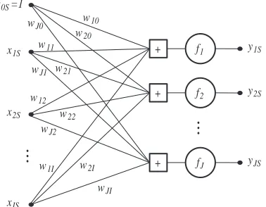
2. One-Layer Neural Networks

Consider the one-layer network in Figure 1. The set of equations relating inputs and outputs is given by

yjs= fj I

∑

i=0 wjixis

!

; j=1,2, . . . ,J; s=1,2, . . . ,S,

where I is the number of inputs, J the number of outputs, x0s=1, wjiare the weights associated

with neuron j and S is the number of data points.

f1

f2

fJ

...

y1S

y2S

yJS

x1S

x2S

xIS

...

w11

w21

wJ1

w12

w22

wJ2

w1I w2I

wJI

wJ0 w10

w20

x0S=1

+

+

+

Figure 1: One-layer feedforward neural network.

To learn the weights wji, the following sum of squared errors between the real and the desired

P=

S

∑

s=1 J

∑

j=1

δ2

js= S

∑

s=1 J

∑

j=1

yjs−fj I

∑

i=0 wjixis

!!2

.

Assuming that the nonlinear activation functions, fj, are invertible (as it is the case for the most

commonly employed functions), alternatively, one can minimize the sum of squared errors before the nonlinear activation functions (Castillo et al., 2002), that is,

Q= ∑S

s=1 J

∑

j=1

ε2

js = S

∑

s=1 J

∑

j=1 _I

∑

i=0

wjixis−f−j 1(yjs) 2

, (1)

which leads to the system of equations:

∂Q

∂wj p

=2

S

∑

s=1 I

∑

i=0

wjixis−fj−1(yjs) !

xps = 0; p=0,1, . . . ,I; ∀j,

that is,

I

∑

i=0 wji

S

∑

s=1

xisxps = S

∑

s=1

f_j−1(yjs)xps; p=0,1, . . . ,I; ∀j

or

I

∑

i=0

Apiwji = bp j; p=0,1, . . . ,I; ∀j, (2)

where

Api = S

∑

s=1

xisxps; p=0,1, . . . ,I; ∀i

bp j = S

∑

s=1

f−_j 1(yjs)xps; p=0,1, . . . ,I; ∀j.

Moreover, for the neural network shown in Figure 1, the sensitivities (see Castillo et al., 2001, 2004, 2006) of the new cost function, Q, with respect to the output and input data can be obtained as:

∂Q

∂ypq

= −

2

_I

∑

i=0

wpixiq−fp−1(ypq)

f′ p(ypq)

; ∀p,q (3)

∂Q

∂xpq

= 2

J

∑

j=1 I

∑

i=0

wjixiq−f−j 1(yjq) !

3. The Proposed Sensitivity-Based Linear Learning Method

The learning method and the sensitivity formulas given in the previous section can be used to de-velop a new learning method for two-layer feedforward neural networks, as it is described below.

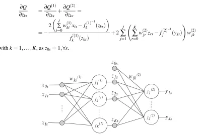
Consider the two-layer feedforward neural network in Figure 2 where I is the number of inputs,

J the number of outputs, K the number of hidden units, x0s=1, z0s=1, S the number of data samples

and the superscripts (1) and(2) are used to refer to the first and second layer, respectively. This

network can be considered to be composed of two one-layer neural networks. Therefore, assuming that the intermediate layer outputs z are known, using equation (1), a new cost function for this network is defined as

Q(z) = Q(1)(z) +Q(2)(z) = =

S

∑

s=1  

K

∑

k=1 I

∑

i=0

w(_ki1)xis−f(1)

−1 k (zks)

!2

+

J

∑

j=1 K

∑

k=0

w(_jk2)zks−f(2)

−1 j (yjs)

!2 .

Thus, using the outputs zks we can learn, for each layer independently, the weights w(_ki1) and

w(_jk2)by solving the corresponding linear system of equations (2). After that, the sensitivities (see equations (3) and (4)) with respect to zksare calculated as:

∂Q

∂zks

=∂Q

(1)

∂zks

+∂Q

(2)

∂zks

=

=−

2

_I

∑

i=0

w(_ki1)xis−f( 1)−1 k (zks)

f_k′(1)(zks)

+2

J

∑

j=1 K

∑

r=0

w(_jr2)zrs−f(2)

−1 j (yjs)

! w(_jk2)

with k=1, . . . ,K, as z0s=1,∀s.

fK(1)

f 2(1) f1(1)

w

f 1(2)

f J(2)

x

x

x

y

y

w

z

z

z

z

Figure 2: Two-layer feedforward neural network.

Next, the values of the intermediate outputs z are modified using the Taylor series approxima-tion:

Q(z+∆z) =Q(z) +

K

∑

k=1 S

∑

s=1

∂Q(z)

∂zks

which leads to the following increments

∆z=−ρ Q(z)

||∇Q||2∇Q, (5)

whereρis a relaxation factor or step size.

The proposed method is summarized in the following algorithm.

Algorithm SBLLM

Input. The data set (input, xis, and desired data, yjs), two threshold errors (ε andε′) to control

convergence, and a step sizeρ.

Output. The weights of the two layers and the sensitivities of the sum of squared errors with

respect to input and output data.

Step 0: Initialization. Assign to the outputs of the intermediate layer the output associated with

some random weights w(1)(0)plus a small random error, that is:

zks=f_k(1) I

∑

i=0

w(_ki1)(0)xis !

+εks; εks∼U(−η,η); k=1, . . . ,K,

where ηis a small number, and initialize Qprevious and MSEprevious to some large number, where

MSE measures the error between the obtained and the desired output.

Step 1: Subproblem solution. Learn the weights of layers 1 and 2 and the associated sensitivities

solving the corresponding systems of equations, that is,

I

∑

i=0

A(_pi1)w(_ki1) = b(_pk1) K

∑

k=0

A_qk(2)w(_jk2) = b(_{q j}2),

where A(_pi1)= ∑S

s=1

xisxps; b(pk1)= S

∑

s=1

f_k(1)−1(zks)xps; p=0,1, . . . ,I; k=1,2, . . . ,K

and A(_qk2)= ∑S

s=1

zkszqs; b(q j2)= S

∑

s=1

f(_j2)−1(yjs)zqs; q=0,1, . . . ,K; ∀j.

Step 2: Evaluate the sum of squared errors. Evaluate Q using

Q(z) =Q(1)(z) +Q(2)(z) =

S

∑

s=1  

K

∑

k=1 I

∑

i=0

w(_ki1)xis−f(1)

−1 k (zks)

!2

+

J

∑

j=1 K

∑

k=0

w(_jk2)zks−f(2)

−1 j (yjs)

!2 

Step 3: Convergence checking. If|Q−Qprevious|<εor|MSEprevious−MSE|<ε′stop and return

the weights and the sensitivities. Otherwise, continue with Step 4.

Step 4: Check improvement of Q. If Q>Qprevious reduce the value ofρ, that is, ρ=ρ/2, and

return to the previous position, that is, restore the weights, z=zprevious, Q=Qpreviousand go to Step

5. Otherwise, store the values of Q and z, that is, Qprevious=Q, MSEprevious=MSE and zprevious=z

and obtain the sensitivities using:

∂Q

∂zks

=−

2

_I

∑

i=0

w(_ki1)xis−f(1)

−1 k (zks)

f_k′(1)(zks)

+2

J

∑

j=1 K

∑

r=0

w(_jr2)zrs−f(2)

−1 j (yjs)

!

w(_jk2); k=1, . . . ,K.

Step 5: Update intermediate outputs. Using the Taylor series approximation in equation (5),

update the intermediate outputs as

z=z−ρ Q(z) ||∇Q||2∇Q

and go to Step 1.

The complexity of this method is determined by the complexity of Step 1 which solves a linear system of equations for each network’s layer. Several efficient methods can be used to solve this

kind of systems with a complexity of O(n2), where n is the number of unknowns. Therefore, the

resulting complexity of the proposed learning method is also O(n2), being n the number of weights

of the network.

4. Examples of Applications of the SBLLM to Train Neural Networks

In this section the proposed method, SBLLM,1 is illustrated by its application to five system

iden-tification problems. Two of them are small/medium size problems (Dow-Jones and Leuven compe-tition time series), while the other three used large data sets and networks (Lorenz time series, and the MNIST and UCI Forest databases). Also, in order to check the performance of the SBLLM, it was compared with five of the most popular learning methods. Three of these methods are the gradient descent (GD), the gradient descent with adaptive momentum and step sizes (GDX), and

the stochastic gradient descent (SGD), whose complexity is O(n). The other methods are the scaled

conjugated gradient (SCG), with complexity of O(n2), and the Levenberg-Marquardt (LM)

(com-plexity of O(n3_{)). All experiments were carried out in MATLAB}R _{running on a Compaq HPC 320}

with an Alpha EV68 1 GHz processor and 4GB of memory. For each experiment all the learning methods shared the following conditions:

• The network topology and neural functions. In all cases, the logistic function was used for

hidden neurons, while for output neurons the linear function was used for regression problems and the logistic function was used for classification problems. It is important to remark that the aim here is not to investigate the optimal topology, but to check the performance of the algorithms in both small and large networks.

• Initial step size equal to 0.05, except for the stochastic gradient descent. In this last case, we

used a step size in the interval [0.005,0.2]. These step sizes were tuned in order to obtain

good results.

• The input data set was normalized (mean = 0 and standard deviation = 1).

• Several simulations were performed using for each one a different set of initial weights. This

initial set was the same for all the algorithms (except for the SBLLM), and was obtained by the Nguyen-Widrow (Nguyen and Widrow, 1990) initialization method.

• Finally, statistical tests were performed in order to check whether the differences in accuracy

and speed were significant among the different training algorithms. Specifically, first the non-parametric Kruskal-Wallis test (Hollander and Wolfe, 1973) was applied to check the hypothesis that all mean performances are equal. When this hypothesis is rejected, a multiple comparison test of means based on the Tukey’s honestly significant difference criterion (Hsu, 1996) was applied to know which pairs of means are different. In all cases, a significance level of 0.05 was used.

4.1 Dow-Jones Time Series

The first data set is the time series corresponding to the Dow-Jones index values for years 1994-1996 (Ley, 1994-1996). The goal of the network in this case is to predict the index for a given day based on the index of five previous days. For this data set a 5-7-1 topology (5 inputs, 7 hidden neurons and 1 output neuron) was used. Also, 900 samples were employed for the learning process. In order to obtain the MSE curves during the learning process 100 simulations of 3000 iterations each, were done.

Figure 3(a) shows, for each method, the mean error curve calculated over the 100 simulations. Also, in Figure 3(b) the box-whisker plots are shown for the 100 MSEs obtained by each method at the end of the training. In this graphic the box corresponds to the interquartile range, the bar inside the box represents the median, the whiskers extend to the farthest points that are not outliers, and outliers are represented by the plus sign.

Also, different measures were calculated and collected in Table 4.1. These measures are:

• M1: Mean and standard deviation of the minimum MSEs obtained by each method over the

100 simulations.

• M2: Mean epoch and corresponding standard deviation in which each of the other methods

reaches the minimum MSE obtained by the SBLLM.

• M3: MSE and standard deviation for each of the other methods at the epoch in which the

SBLLM gets its minimum.

In this case, the best mean MSE is achieved by the LM method (see M1 in Table 4.1). Also,

applying the multiple comparison test, it was found that the difference between this mean and those from the others methods was statistically significant.

Finally, the mean CPU times and the corresponding standard deviations for each of the methods

are shown in Table 4.1. In this table, the variables tepochmean and tepochstd are the mean and

ttotalstd correspond to the mean and standard deviation of the time needed to reach the minimum

MSE. The Ratio column contains the relation between the ttotalmean of each algorithm and the

fastest one. Again, the multiple comparison test applied over the ttotalmeanrevealed that the speed

of the fastest method, that is the SBLLM, was only comparable to that of the SCG.

100

101

102

103

104

10−4

10−3

10−2

10−1

100

101

Epoch

Mean MSE

SBLLM LM

SGD

SCG GDX GD

(a) Mean error curves over 100 simulations

GD SCG GDX LM SBLLM SGD 0

0.01 0.02 0.03 0.04 0.05 0.06

MSE

(b) Boxplot of the 100 MSE values obtained at the end of the training

Figure 3: Results of the learning process for the Dow-Jones data.

M1 M2 M3

SBLLM 4.866×10−4±2.252×10−6 2.08±0.394 4.866×10−4±2.252×10−6

LM 4.601×10−4±1.369×10−5 20±11.5 9.099×10−2±2.190×10−1

SCG 1.928×10−3±8.959×10−3 354±150(∗1) 5.517×10−2±6.034×10−3

GDX 7.747×10−3±1.802×10−2 2,180±635(∗2) 4.717×10−1±5.962×10−1

GD 2.020×10−2±2.369×10−2 >3000 5.517×10−2±5.950×10−1

SGD 5.995×10−2±1.360×10−3 >3000 9.001×10−2±1.356×10−2

(∗1)4% of the curves did not get the minimum of SBLLM (∗2)99.5% of the curves did not get the minimum of SBLLM

Table 1: Comparative measures for the Dow-Jones data.

tepochmean tepochstd ttotalmean ttotalstd Ratio

GD 0.0077 9.883×10−5 23.125 0.297 223.4

GDX 0.0078 1.548×10−4 22.764 3.548 219.9

SBLLM 0.0089 1.600×10−3 0.104 0.115 1

SCG 0.0165 2.800×10−3 15.461 8.595 149.4

LM 0.0395 3.460×10−2 115.619 106.068 1,117.1

SGD 0.2521 1.814×10−3 756.570 5.445 7,274.7

4.2 K.U. Leuven Competition Data

The K.U. Leuven time series prediction competition data (Suykens and Vandewalle, 1998) were generated from a computer simulated 5-scroll attractor, resulting from a generalized Chua’s circuit which is a paradigm for chaos. 1800 data points of this time series were used for training. The aim of the neural network is to predict the current sample using only 4 previous data points. Thus the training set is reduced to 1796 input patterns corresponding to the number of 4-samples sliding windows over the initial training set. For this problem a 4-8-1 topology was used. As for the previous experiment 100 simulations of 3000 iterations each were carried out. Results are shown in Figure 4, and Tables 4.2 and 4.2.

In this case, the best mean MSE is achieved by the LM method (see M1in Table 4.2). However,

the multiple comparison test did not show any significant difference with respect to the means of

the SCG and the SBLLM. Regarding the ttotalmean, the multiple comparison test showed that the

speed of the fastest method, that is the SBLLM, was only comparable to those of the GDX and the GD.

100

101

102

103

104

10−5

10−4

10−3

10−2

10−1

100

101

Epoch

Mean MSE

SBLLM LM

SGD SCG

GDX GD

(a) Mean error curves over 100 simulations

GD SCG GDX LM SBLLM SGD 10−4

10−3

MSE

(b) Boxplot of the 100 MSE values obtained at the end of the training

Figure 4: Results of the learning process for the Leuven competition data.

M1 M2 M3

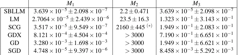
SBLLM 3.639×10−5±2.098×10−7 2.2±0.471 3.639×10−5±2.098×10−7

LM 2.7064×10−5±2.439×10−6 23.5±16.3 1.323×10−1±3.143×10−1

SCG 3.517×10−5±9.549×10−7 2160±445(∗) 1.949×10−1±2.083×10−1

GDX 8.121×10−4±4.504×10−4 >3000 7.190×10−1±6.651×10−1

GD 3.280×10−3±1.698×10−3 >3000 1.949×10−1±6.621×10−1

SGD 4.748×10−5±9.397×10−6 >3000 8.458×10−3±5.292×10−3

(∗)9.8% of the curves did not get the minimum of SBLLM

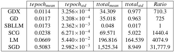
tepochmean tepochstd ttotalmean ttotalstd Ratio

GDX 0.0114 3.256×10−4 34.309 0.977 710.3

GD 0.0117 3.208×10−4 35.018 0.963 725

SBLLM 0.0173 2.362×10−3 0.048 0.017 1

SCG 0.0238 6.271×10−4 69.571 5.022 1440.4

LM 0.0669 5.440×10−2 196.816 164.539 4074.9

SGD 0.5083 2.982×10−3 1,525.34 8.949 31,777.9

Table 4: CPU time comparison for the Leuven competition data.

4.3 Lorenz Time Series

A Lorenz system (Lorenz, 1963) is described by the solution of three simultaneous differential equations:

dx/dt=−σx+σy

dy/dt=−xz+rx−y

dz/dt=xy−bz,

whereσ, r and b are constants. For this work, we employedσ=10, r=28, and b=8/3, for which

the system presents a chaotic dynamics. The goal of the network is to predict the current sample based on the four previous samples. For this data set a 8-100-1 topology was used. Also, 150000 samples were employed for the learning process. In this case, and due to the large size of both the data set and the neural networks, the conditions of the experiments were the following:

• The number of simulations, which were carried out to obtain the MSE curves during the

learning process was reduced to 30, of 1000 iterations each.

• Neither the GD nor the LM methods were used. The results of the GD will not be presented

because the method performed poorly, and the LM is impractical in these cases as it is highly computationally demanding (LeCun et al., 1998).

100

101

102

103

10−8

10−7

10−6

10−5

10−4

10−3

10−2

10−1

100

101

102

Epoch

Mean MSE

SBLLM

SGD SCG

GDX

(a) Mean error curves over 30 simulations

SCG GDX SBLLM SGD 10−7

10−6

10−5

10−4

10−3

MSE

(b) Boxplot of the 30 MSE values obtained at the end of the training

Figure 5: Results of the learning process for the Lorenz data.

M1 M2 M3

SBLLM 3.118×10−8±2.151×10−8 2.47±0.776 3.118×10−8±2.151×10−8

SGD 1.426×10−6±2.710×10−7 >1000 2.512×10−2±1.345×10−2

SCG 1.545×10−5±3.922×10−6 >1000 1.286×101±5.538

GDX 3.774×10−3±8.409×10−4 >1000 7.722×101±1.960×101

Table 5: Comparative measures for the Lorenz data.

tepochmean tepochstd ttotalmean ttotalstd Ratio

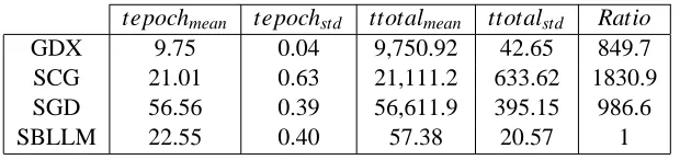
GDX 9.75 0.04 9,750.92 42.65 849.7

SCG 21.01 0.63 21,111.2 633.62 1830.9

SGD 56.56 0.39 56,611.9 395.15 986.6

SBLLM 22.55 0.40 57.38 20.57 1

Table 6: CPU time comparison for the Lorenz data.

4.4 MNIST Data Set

The MNIST database, available at http://yann.lecun.com/exdb/mnist/, contains grey level images of

handwritten digits of 28×28 pixels. It is a real classification problem whose goal is to determine

the written number which is always an integer in the range between 0 and 9. This database is originally divided into a training set of 60,000 examples, and a test set of 10,000 examples. Further we extracted 10,000 samples from the training set to be used as a validation set.

For this data set we used 784 inputs neurons fed by the 28×28 pixels of each input pattern, and

one output neuron per class. Specifically a 784-800-10 topology was used. In this case, and due to the large size of both the data set and the neural network, the conditions of the experiments were the following:

• The number of simulations, which were carried out to obtain the classification error was

• Allowing a maximum of 200 iterations per simulation, the early stopping criteria using the validation set was employed to halt learning.

• The LM method was not used, since it is impractical in these cases as it is highly

computa-tionally demanding (LeCun et al., 1998).

• Concerning the other batch methods only the SCG was used since it is the one that clearly

obtains the best results and convergence speed in the previous experiments.

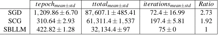
Results are shown in Tables 4.4 and 4.4. As mentioned, the training process of the three methods were halted using the stop learning criteria. In this case, as can be observed the SGD achieved the best mean test accuracy, confirmed by the multiple comparison test. Besides, in all simulations the SBLLM always stops in iteration 75 achieving a worse accuracy than the SGD but employing a total time lesser than the other methods. In order to check if this result could be improved we did some other experiments allowing the SBLLM to run as long as the Stochastic Gradient Descent (SGD). However, results were not improved. Therefore, the presented tables show the most favourable situation for each algorithm.

Regarding the total CPU time, again the fastest method is the SBLLM, with a ttotalmean

signifi-cantly different from the other two methods.

Trainmean±std Validationmean±std Testmean±std

SGD 99.93±0.04 97.87±0.09 97.70±0.08

SCG 78.12±22.46 77.21±21.97 77.03±22.05

SBLLM 85.73±0.03 86.52±0.15 86.08±0.26

Table 7: Classification accuracy for the MNIST data.

tepochmean±std ttotalmean±std iterationsmean±std Ratio

SGD 1,209.86±6.70 87,607.1±485.41 72.4±16.99 2.73

SCG 310.64±2.93 61,311.4±1,537 197.4±5.81 1.92

SBLLM 422.82±1.28 32,134.4±97 75±0 1

Table 8: CPU time comparison for the MNIST data.

4.5 Forest

The Forest CoverType database, on-line at http://kdd.ics.uci.edu/databases/covertype/covertype.html,

contains data describing the wilderness areas and soil types for 30×30 meter cells obtained from US

For this data set a 54-500-2 topology was used. Regarding the number of simulations, stopping criteria and learning methods, the conditions were the same as those of the MNIST experiment described in the previous section.

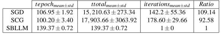
As in the previous section, the most favourable results for each algorithm are shown in Tables 4.5 and 4.5. In this data set, the SGD achieved the best mean test accuracy, confirmed by the multiple comparison test. Regarding the total CPU time, the fastest method is the SBLLM, with a

ttotalmeansignificantly different from the other two methods. It is important to remark that although

in this case the SBLLM is the fastest method, this is due to the stop of the learning process in an early stage. This does not allow the SBLLM to achieve a good accuracy, as it is shown in Table 4.5. These results confirm that, for classification problems the SGD seems to be better in error than the SBLLM, which is similar in error but faster than the SCG.

Trainmean±std Validationmean±std Testmean±std

SGD 89.60±0.92 88.21±0.69 88.22±0.56

SCG 79.03±1.29 78.69±1.15 79.08±1.16

SBLLM 79.87±1.05 79.65±0.22 79.92±0.15

Table 9: Classification accuracy for the forest cover type data.

tepochmean±std ttotalmean±std iterationsmean±std Ratio

SGD 106.95±1.92 15,210.63±273.34 142.2±55.36 109.14

SCG 100.20±3.40 17,903.66±3063.92 178.60±29.66 92.58

SBLLM 139.37±0.72 139.37±0.72 1±0 1

Table 10: CPU time comparison for the forest cover type data.

5. The SBLLM as Initialization Method

As has been shown in the previous section, the SBLLM achieves a small error rate in very few epochs. Although this error rate is very small and, in general, better than the errors obtained by other learning methods, as can be seen in Figures 3(a), 4(a) and 5(a), once the SBLLM gets this point the variation in the MSE in further epochs is not significant. For this reason, an interesting alternative is to combine the SBLLM with other learning methods.

In this section, the results of the SBLLM used as an initialization method instead of as a learning algorithm are presented. Thus, several experiments were accomplished using the SBLLM only to get the initial values of the weights of the neural network. Afterwards, the LM and SCG were used as learning methods from these initial values. The experiments were carried out using the Dow-Jones, Leuven and Lorenz time series. For these three data sets the experimental conditions were the same as those described in Section 4.

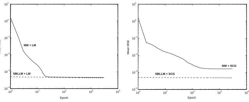
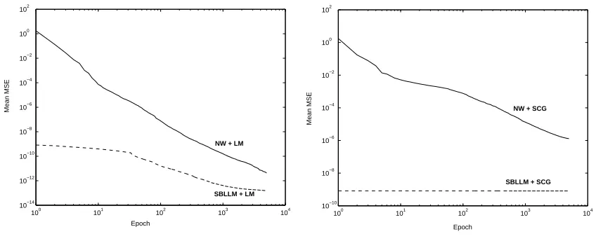
Figures 6(a), 7(a) and 8(a) show the corresponding mean curves (over the 100 simulations) of the learning process using the SBLLM and the NW as initialization methods and the LM as the learning algorithm. Figures 6(b), 7(b) and 8(b) show the same mean curves of the learning process using this time the SCG as learning algorithm.

100

101

102

103

104 10−4

10−3 10−2 10−1 100 101

Epoch

Mean MSE

NW + LM

SBLLM + LM

(a) Mean error curves for the LM method

100 101 102 103 104

10−4 10−3 10−2 10−1 100 101

Epoch

Mean MSE

NW + SCG

SBLLM + SCG

(b) Mean error curves for the SCG method

Figure 6: Mean error curves over 100 simulations for the Dow-Jones time series using the SBLLM and the NW as initialization methods.

100 101 102 103 104

10−5 10−4 10−3 10−2 10−1 100 101

Epoch

Mean MSE

NW + LM

SBLLM + LM

(a) Mean error curves for the LM method

100 101 102 103 104

10−5 10−4 10−3 10−2 10−1 100 101

Epoch

Mean MSE

NW + SCG

SBLLM + SCG

(b) Mean error curves for the SCG method

100 101 102 103 104 10−14

10−12 10−10 10−8 10−6 10−4 10−2 100 102

Mean MSE

NW + LM

SBLLM + LM

Epoch

(a) Mean error curves for the LM method

100 101 102 103 104

10−10 10−8 10−6 10−4 10−2 100 102

Epoch

Mean MSE

NW + SCG

SBLLM + SCG

(b) Mean error curves for the SCG method

Figure 8: Mean error curves over 100 simulations for the Lorenz time series using the SBLLM and the NW as initialization methods.

Figures 9(a), 10(a) and 11(a) contain the boxplots of the methods in the last epoch of training (3000) using the SBLLM and NW as initialization methods and the LM as the learning algorithm. Figures 9(b), 10(b) and 11(b) depict the same boxplots when using the SCG as the learning algo-rithm.

NW + LM SBLLM + LM

4.3 4.4 4.5 4.6 4.7 4.8

x 10−4

MSE

(a) Boxplot for the LM method

NW + SCG SBLLM + SCG 4.7

4.75 4.8 4.85

x 10−4

MSE

(b) Boxplot for the SCG method

NW + LM SBLLM + LM 2.2

2.3 2.4 2.5 2.6 2.7 2.8 2.9 3 3.1

x 10−5

MSE

(a) Boxplot for the LM method

NW + SCG SBLLM + SCG 3.2

3.4 3.6 3.8 4 4.2 4.4 4.6

x 10−5

MSE

(b) Boxplot for the SCG method

Figure 10: Boxplot of the 100 MSE values at the last epoch of training for the Leuven competition time series using the SBLLM and NW as initialization methods.

NW + LM SBLLM + LM

0 1 2 3 4 5 6 7

x 10−11

MSE

(a) Boxplot for the LM method

NW + SCG SBLLM + SCG 0

0.5 1 1.5 2 2.5 3 3.5

x 10−6

MSE

(b) Boxplot for the SCG method

Figure 11: Boxplot of the 100 MSE values at the last epoch of training for the Lorenz time series using the SBLLM and NW as initialization methods.

6. Discussion

Regarding the behavior of the SBLLM as a learning algorithm, and from the experiments made and the results presented in Section 4, there are three main features of the SBLLM that stand out:

1. High speed in reaching the minimum error. For the first three problems (Dow-Jones, Leuven and Lorenz time series), this feature can be observed in Figures 3(a), 4(a) and 5(a), and the

obtains its minimum MSE (minMSE) just before the first 4 iterations and also sooner than

the rest of the algorithms. Moreover, and generally speaking, measure M3 reflects that the

SBLLM gets its minimum in an epoch for which the other algorithms are far from similar MSE values.

If we take into account the CPU times in Tables 4.1, 4.2, 4.3, 4.4 and 4.5 we can see that, as expected, the CPU time per epoch of the SBLLM is similar to that of the SCG (both of

O(n2)), and when we consider the total CPU time per simulation the SBLLM is, in the worst

case, more than 150 times faster than the fastest algorithm for the regression examples and approximately 2 times faster for the classification examples. It is also important to remark that despite of the advantages of the LM method, it could not be applied in the experiments that involved large data sets and neural networks as it is impractical for such cases (LeCun et al., 1998).

2. A good performance. From Figures 3(a), 4(a) and 5(a), and the measure M1in Tables 4.1, 4.2

and 4.3, it can be deduced that not only the SBLLM stabilizes soon, but also the minMSE that it reaches is quite good and comparable to that obtained by the second order methods. On the other hand, the GD and the GDX learning methods never succeeded in attaining this minMSE

before the maximum number of epochs, as reflected in measure M2(Tables 4.1, 4.2 and 4.3).

Finally, the SCG algorithm presents an intermediate behavior, although seldom achieves the levels of performance of the LM and SBLLM.

Regarding the classification problems, from Tables 4.4 and 4.5, it can be deduced that the SBLLM performs similar or better than the other batch method, that is the SCG, while the stochastic method (SGD) is the best algorithm for this kind of problems (LeCun et al., 1998).

Although the ability of the proposed algorithm to get a minimum in just very few epochs is usually an advantage, it can also be noticed that once it achieves this minimum (local or global) it gets stuck in this point. This causes that, sometimes like in the classification examples included, the algorithm is not able to obtain a high accuracy. This behavior could be explained by the initialization method and the updating rule for the step size employed.

3. Homogeneous behavior. This feature comprehends several aspects:

• The SBLLM learning curve stabilizes soon, as can be observed in Figures 3(a), 4(a) and

5(a).

• Regarding the minimum MSE reached at the end of the learning process, it can be

observed from Figures 3(b), 4(b) and 5(b) that, in any case, the GD and GDX algorithms present a wider dispersion, given even place to the appearance of outliers. On the other hand, the SGD, SCG, LM and SBLLM algorithms tend to always obtain nearer values

of MSE. This fact is also reflected by the standard deviations of measure M1.

• The SBLLM behaves homogeneously not only if we consider just the end of the learning

process, as commented, but also during the whole process, in such a way that very sim-ilar learning curves where obtained for all iterations of the first three experiments. This

is, in a certain way, reflected in the standard deviation of measure M3which corresponds

• Finally, from Tables 4.4 and 4.5 it can be observed that for these last two experiments (MNIST and Forest databases) this homogeneus behaviour stands for the SGD and the SBLLM, while the SCG presents a wider dispersion in its classification errors.

With respect to the use of the SBLLM as initialization method, as it can be observed in Figures 6, 7 and 8, the SBLLM combined with the LM or the SCG achieves a faster convergence speed than the same methods using the NW as initialization method. Also, the SBLLM obtains a very good initial point, and thus a very low MSE in a few epochs of training. Moreover, in this case, most of the times the final MSE achieved is smaller than the one obtained using the NW initialization method. This result is better illustrated in the boxplots of the corresponding time series where it can be observed, in addition, that the final MSE obtained with NW presents a higher variability than that achieved by the SBLLM, that is, the SBLLM helps the learning algorithms to obtain a more homogeneous MSE at the end of the training process. Thus, experiments confirm the utility of the SBLLM as an initialization method, which effect is to speed up the convergence.

7. Conclusions and Future Work

The main conclusions that can be drawn from this paper are:

1. The sensitivities of the sum of squared errors with respect to the outputs of the intermediate layer allow an efficient and fast gradient method to be applied.

2. Over the experiments made the SBLLM offers an interesting combination of speed, reliability and simplicity.

3. Regarding the employed regression problems only second order methods, and more specifi-cally the LM, seem to obtain similar results although at a higher computational cost.

4. With respect to the employed classification problems, the SBLLM performs similar or bet-ter than the other batch method, although requiring less computational time. Besides, the stochastic gradient (SGD) is the one that obtains the lowest classification error. This result is in accordance with that obtained by other authors (LeCun et al., 1998) that recommend this method for large data sets and networks in classification tasks.

5. The SBLLM used as an initialization method significantly improves the performance of a learning algorithm.

Finally, there are some aspects of the proposed algorithm that need an in depth study, and will be addressed in a future work:

1. A more appropriate method to set the initial values of the outputs z of hidden neurons (step 0 of the proposed algorithm).

2. A more efficient updating rule for the step sizeρ, like a method based on a line search (hard

or soft).

Acknowledgments

We would like to acknowledge support for this project from the Spanish Ministry of Science and Technology (Projects DPI2002-04172-C04-02 and TIC2003-00600, this last partially supported by FEDER funds) and the Xunta de Galicia (project PGIDT04PXIC10502PN). Also, we thank the Supercomputing Center of Galicia (CESGA) for allowing us the use of the high performance com-puting servers.

References

L. B. Almeida, T. Langlois, J. D. Amaral, and A. Plakhov. Parameter adaptation in stochastic optimization. In D. Saad, editor, On-line Learning in Neural Networks, chapter 6, pages 111– 134. Cambridge University Press, 1999.

R. Battiti. First and second order methods for learning: Between steepest descent and Newton’s method. Neural Computation, 4(2):141–166, 1992.

E. M. L. Beale. A derivation of conjugate gradients. In F. A. Lootsma, editor, Numerical methods

for nonlinear optimization, pages 39–43. Academic Press, London, 1972.

F. Biegler-K¨onig and F. B¨armann. A learning algorithm for multilayered neural networks based on linear least-squares problems. Neural Networks, 6:127–131, 1993.

W. L. Buntine and A. S. Weigend. Computing second derivatives in feed-forward networks: A review. IEEE Transactions on Neural Networks, 5(3):480–488, 1993.

E. Castillo, J. M. Guti´errez, and A. Hadi. Sensitivity analysis in discrete bayesian networks. IEEE

Transactions on Systems, Man and Cybernetics, 26(7):412–423, 1997.

E. Castillo, A. Cobo, J. M. Guti´errez, and R. E. Pruneda. Working with differential, functional and difference equations using functional networks. Applied Mathematical Modelling, 23(2):89–107, 1999.

E. Castillo, A. Cobo, J. M. Guti´errez, and R. E. Pruneda. Functional networks. a new neural network based methodology. Computer-Aided Civil and Infrastructure Engineering, 15(2):90–106, 2000.

E. Castillo, A. Conejo, P. Pedregal, R. Garc´ıa, and N. Alguacil. Building and Solving Mathematical

Programming Models in Engineering and Science. John Wiley & Sons Inc., New York., 2001.

E. Castillo, O. Fontenla-Romero, A. Alonso Betanzos, and B. Guijarro-Berdi˜nas. A global optimum approach for one-layer neural networks. Neural Computation, 14(6):1429–1449, 2002.

E. Castillo, A. S. Hadi, A. Conejo, and A. Fern´andez-Canteli. A general method for local sensitivity analysis with application to regression models and other optimization problems. Technometrics, 46(4):430–445, 2004.

A. Chella, A. Gentile, F. Sorbello, and A. Tarantino. Supervised learning for feed-forward neural networks: a new minimax approach for fast convergence. Proceedings of the IEEE International

Conference on Neural Networks, 1:605 – 609, 1993.

V. Cherkassky and F. Mulier. Learning from Data: Concepts, Theory, and Methods. Wiley, New York, 1998.

R. Collobert, Y. Bengio, and S. Bengio. Scaling large learning problems with hard parallel mixtures.

International Journal of Pattern Recognition and Artificial Intelligence, 17(3):349–365, 2003.

J. E. Dennis and R. B. Schnabel. Numerical Methods for Unconstrained Optimization and Nonlinear

Equations. Prentice-Hall, Englewood Cliffs, NJ, 1983.

G. P. Drago and S. Ridella. Statistically controlled activation weight initialization (SCAWI). IEEE

Transactions on Neural Networks, 3:899–905, 1992.

R. Fletcher and C. M. Reeves. Function minimization by conjugate gradients. Computer Journal, 7 (149–154), 1964.

O. Fontenla-Romero, D. Erdogmus, J.C. Principe, A. Alonso-Betanzos, and E. Castillo. Linear least-squares based methods for neural networks learning. Lecture Notes in Computer Science, 2714(84–91), 2003.

M. T. Hagan and M. Menhaj. Training feedforward networks with the marquardt algorithm. IEEE

Transactions on Neural Networks, 5(6):989–993, 1994.

M. T. Hagan, H. B. Demuth, and M. H. Beale. Neural Network Design. PWS Publishing, Boston, MA, 1996.

M. Hollander and D. A. Wolfe. Nonparametric Statistical Methods. John Wiley & Sons, 1973.

J. C. Hsu. Multiple Comparisons. Theory and Methods. Chapman&Hall/CRC, Boca Raton, FL, 1996.

D. R. Hush and J. M. Salas. Improving the learning rate of back-propagation with the gradient reuse algorithm. Proceedings of the IEEE Conference of Neural Networks, 1:441–447, 1988.

B. C. Ihm and D. J. Park. Acceleration of learning speed in neural networks by reducing weight oscillations. Proceedings of the International Joint Conference on Neural Networks, 3:1729– 1732, 1999.

R. A. Jacobs. Increased rates of convergence through learning rate adaptation. Neural Networks, 1 (4):295–308, 1988.

Y. LeCun, I. Kanter, and S.A. Solla. Second order properties of error surfaces: Learning time and generalization. In R.P. Lippmann, J.E. Moody, and D.S. Touretzky, editors, Neural Information

Processing Systems, volume 3, pages 918–924, San Mateo, CA, 1991. Morgan Kaufmann.

K. Levenberg. A method for the solution of certain non-linear problems in least squares. Quaterly

Journal of Applied Mathematics, 2(2):164–168, 1944.

E. Ley. On the peculiar distribution of the U.S. stock indeces’ first digits. The American Statistician, 50(4):311–314, 1996.

E. N. Lorenz. Deterministic nonperiodic flow. Journal of the Atmospheric Sciences, 20:130–141, 1963.

D. W. Marquardt. An algorithm for least-squares estimation of non-linear parameters. Journal of

the Society of Industrial and Applied Mathematics, 11(2):431–441, 1963.

M. F. Moller. A scaled conjugate gradient algorithm for fast supervised learning. Neural Networks, 6:525–533, 1993.

D. Nguyen and B. Widrow. Improving the learning speed of 2-layer neural networks by choosing initial values of the adaptive weights. Proceedings of the International Joint Conference on

Neural Networks, 3:21–26, 1990.

G. B. Orr and T. K. Leen. Using curvature information for fast stochastic search. In M.I. Jordan, M.C. Mozer, and T. Petsche, editors, Neural Information Processing Systems, volume 9, pages 606–612, Cambridge, 1996. MIT Press.

D. B. Parker. Optimal algorithms for adaptive networks: second order back propagation, second order direct propagation, and second order hebbian learning. Proceedings of the IEEE Conference

on Neural Networks, 2:593–600, 1987.

S. Pethel, C. Bowden, and M. Scalora. Characterization of optical instabilities and chaos using MLP training algorithms. SPIE Chaos Opt., 2039:129–140, 1993.

M. J. D. Powell. Restart procedures for the conjugate gradient method. Mathematical Programming, 12:241–254, 1977.

S. Ridella, S. Rovetta, and R. Zunino. Circular backpropagation networks for classification. IEEE

Transactions on Neural Networks, 8(1):84–97, January 1997.

A. K. Rigler, J. M. Irvine, and T. P. Vogl. Rescaling of variables in back propagation learning.

Neural Networks, 4:225–229, 1991.

D. E. Rumelhart, G. E. Hinton, and R. J. Willian. Learning representations of back-propagation errors. Nature, 323:533–536, 1986.

N. N. Schraudolph. Fast curvature matrix-vector products for second order gradient descent. Neural

Computation, 14(7):1723–1738, 2002.

A. Sperduti and S. Antonina. Speed up learning and network optimization with extended back propagation. Neural Networks, 6:365–383, 1993.

T. Tollenaere. Supersab: Fast adaptive back propagation with good scaling properties. Neural

Networks, 3(561–573), 1990.

T. P. Vogl, J. K. Mangis, A. K. Rigler, W. T. Zink, and D. L. Alkon. Accelerating the convergence of back-propagation method. Biological Cybernetics, 59:257–263, 1988.

M. K. Weir. A method for self-determination of adaptive learning rates in back propagation. Neural

Networks, 4:371–379, 1991.

B. M. Wilamowski, S. Iplikci, O. Kaynak, and M. O. Efe. An algorithm for fast convergence in training neural networks. Proceedings of the International Joint Conference on Neural Networks, 2:1778–1782, 2001.