Fourier Theoretic Probabilistic Inference over Permutations
Jonathan Huang [email protected]
Robotics Institute
Carnegie Mellon University Pittsburgh, PA 15213
Carlos Guestrin [email protected]
Machine Learning Department Carnegie Mellon University Pittsburgh, PA 15213
Leonidas Guibas [email protected]
Department of Computer Science Stanford University
Stanford, CA 94305
Editor: Marina Meila
Abstract
Permutations are ubiquitous in many real-world problems, such as voting, ranking, and data asso-ciation. Representing uncertainty over permutations is challenging, since there are n! possibilities, and typical compact and factorized probability distribution representations, such as graphical mod-els, cannot capture the mutual exclusivity constraints associated with permutations. In this paper, we use the “low-frequency” terms of a Fourier decomposition to represent distributions over per-mutations compactly. We present Kronecker conditioning, a novel approach for maintaining and updating these distributions directly in the Fourier domain, allowing for polynomial time bandlim-ited approximations. Low order Fourier-based approximations, however, may lead to functions that do not correspond to valid distributions. To address this problem, we present a quadratic program defined directly in the Fourier domain for projecting the approximation onto a relaxation of the polytope of legal marginal distributions. We demonstrate the effectiveness of our approach on a real camera-based multi-person tracking scenario.
Keywords: identity management, permutations, approximate inference, group theoretical
meth-ods, sensor networks
1. Introduction
Probability distributions over permutations arise in a diverse variety of real world problems. While they were perhaps first studied in the context of gambling and card games, they have now been found to be applicable to many important problems such as multi-object tracking, information retrieval, webpage ranking, preference elicitation, and voting. Probabilistic reasoning problems over permu-tations, however, are not amenable to the typical representations afforded by machine learning such as Bayesian networks and Markov random fields. This paper explores an alternative representation and inference algorithms based on Fourier analysis for dealing with permutations.
A or B?
A or B? A
B
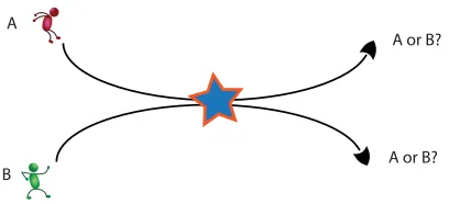
Figure 1: When two persons pass near each other, their identities can get confused.
with an identity corresponding to each track, in spite of ambiguities arising from imperfect identity measurements. When the people are well separated, the problem is easily decomposed and mea-surements about each individual can be clearly associated with a particular track. When people pass near each other, however, confusion can arise as their signal signatures may mix; see Figure 1. Af-ter the individuals separate again, their positions may be clearly distinguishable, but their identities can still be confused, resulting in identity uncertainty which must be propagated forward in time with each person, until additional observations allow for disambiguation. This task of maintaining a belief state for the correct association between object tracks and object identities while accounting for local mixing events and sensor observations, was introduced in Shin et al. (2003) and is called the identity management problem.
The identity management problem poses a challenge for probabilistic inference because it needs to address the fundamental combinatorial challenge that there is a factorial number of associations to maintain between tracks and identities. Distributions over the space of all permutations require storing at least n!−1 numbers, an infeasible task for all but very small n. Moreover, typical com-pact representations, such as graphical models, cannot efficiently capture the mutual exclusivity constraints associated with permutations.
While there have been many approaches for coping with the factorial complexity of maintaining a distribution over permutations, most attack the problem using one of two ideas—storing and up-dating a small subset of likely permutations, or, as in our case, restricting consideration to a tractable subspace of possible distributions. Willsky (1978) was the first to formulate the probabilistic filter-ing/smoothing problem for group-valued random variables. He proposed an efficient FFT based approach of transforming between primal and Fourier domains so as to avoid costly convolutions, and provided efficient algorithms for dihedral and metacyclic groups. Kueh et al. (1999) show that probability distributions on the group of permutations are well approximated by a small subset of Fourier coefficients of the actual distribution, allowing for a principled tradeoff between accuracy and complexity. The approach taken in Shin et al. (2005), Schumitsch et al. (2005), and Schumitsch et al. (2006) can be seen as an algorithm for maintaining a particular fixed subset of Fourier coef-ficients of the log density. Most recently, Kondor et al. (2007) allow for a general set of Fourier coefficients, but assume a restrictive form of the observation model in order to exploit an efficient FFT factorization.
In the following, we outline our main contributions and provide a roadmap of the sections ahead.1
• In Sections 4 and 5, we provide a gentle introduction to the theory of group representations and noncommutative Fourier analyis. While none of the results of these sections are novel, and have indeed been studied by mathematicians for decades (Diaconis, 1989; Terras, 1999; Willsky, 1978; Chen, 1989), noncommutative Fourier analysis is still fairly new to the ma-chine learning community, which has just begun to discover some of its exciting applica-tions (Huang et al., 2007, 2009; Kondor et al., 2007; Kondor and Borgwardt, 2008). Our tutorial sections are targeted specifically at the machine learning community and describe its connections to probabilistic inference problems that involve permutations.
• In Section 6, we discuss performing probabilistic inference operations in the Fourier domain. In particular, we present Fourier theoretic algorithms for two ubiquitous operations which appear in filtering applications and beyond: prediction/rollup and conditioning with Bayes rule. Our main contribution in this section is a novel and conceptually simple algorithm, called Kronecker Conditioning, which performs all conditioning operations completely in the Fourier domain, allowing for a principled tradeoff between computational complexity and approximation accuracy. Our approach generalizes upon previous work in two ways— first, in the sense that it can address any transition model or likelihood function that can be represented in the Fourier domain, and second, in the sense that many of our results hold for arbitrary finite groups.
• In Section 7, we analyze the errors which can be introduced by bandlimiting a probability
distribution and show how they propagate with respect to inference operations. We argue that approximate conditioning based on bandlimited distributions can sometimes yield Fourier coefficients which do not correspond to any valid distribution, even returning negative “prob-abilities” on occasion. We address possible negative and inconsistent probabilities by present-ing a method for projectpresent-ing the result back into the polytope of coefficients which correspond to nonnegative and consistent marginal probabilities using a simple quadratic program.
• In Section 8, we present a collection of general techniques for efficiently computing the
Fourier coefficients of probabilistic models that might be useful in practical inference prob-lems, and give a variety of examples of such computations for probabilistic models that might arise in identity management or ranking scenarios.
• Finally in Section 10, we empirically evaluate the accuracy of approximate inference on sim-ulated data drawn from our model and further demonstrate the effectiveness of our approach on a real camera-based multi-person tracking scenario.
2. Filtering Over Permutations
As a prelude to the general problem statement, we begin with a simple identity management problem on three tracks (illustrated in Figure 2) which we will use as a running example. In this problem, we observe a stream of localization data from three people walking inside a room. Except for a camera positioned at the entrance, however, there is no way to distinguish between identities once they are inside. In this example, an internal tracker declares that two tracks have ‘mixed’ whenever they get too close to each other and announces the identity of any track that enters or exits the room.
(a) Be f ore (b) A f ter
Figure 2: Identity Management example. Three people, Alice, Bob and Charlie enter a room and we receive a position measurement for each person at each time step. With no way to observe identities inside the room, however, we are confused whenever two tracks get too close. In this example, track 1 crosses with track 2, then with track 3, then leaves the room, at which point it is observed that the identity at Track 1 is in fact Bob.
recorded in Table 1. Since Tracks 2 and 3 never mix, we know that Cathy cannot be in Track 2 in the end, and furthermore, since we observe Bob to be in Track 1 when he exits, we can deduce that Cathy must have been in Track 3, and therefore Alice must have been in Track 2. Our simple example illustrates the combinatorial nature of the problem—in particular, reasoning about the mixing events allows us to exactly decide where Alice and Cathy were even though we only made an observation about Bob at the end.
Event # Event Type
1 Tracks 1 and 2 mixed
2 Tracks 1 and 3 mixed
3 Observed Identity Bob at Track 1
Table 1: Table of Mixing and Observation events logged by the tracker.
In identity management, a permutationσrepresents a joint assignment of identities to internal tracks, withσ(i) being the track belonging to the ith identity. When people walk too closely to-gether, their identities can be confused, leading to uncertainty over σ. To model this uncertainty, we use a Hidden Markov Model (HMM) on permutations, which is a joint distribution over latent permutationsσ(1), . . . ,σ(T), and observed variables z(1), . . . ,z(T)which factors as:
P(σ(1), . . . ,σ(T),z(1), . . . ,z(T)) =P(σ(1))P(z(1)|σ(1)) T
∏
t=2P(zt|σ(t))·P(σ(t)|σ(t−1)).
The conditional probability distribution P(σ(t)|σ(t−1))is called the transition model, and might
We focus on filtering, in which one queries the HMM for the posterior at some time step, con-ditioned on all past observations. Given the distribution P(σ(t)|z(1), . . . ,z(t)), we recursively com-pute P(σ(t+1)|z(1), . . . ,z(t+1)) in two steps: a prediction/rollup step and a conditioning step. Taken
together, these two steps form the well known Forward Algorithm (Rabiner, 1989). The predic-tion/rollup step multiplies the distribution by the transition model and marginalizes out the previous time step:
P(σ(t+1)|z(1), . . . ,z(t)) =
∑
σ(t)
P(σ(t+1)|σ(t))P(σ(t)|z(1), . . . ,z(t)).
The conditioning step conditions the distribution on an observation z(t+1)using Bayes rule:
P(σ(t+1)|z(1), . . . ,z(t+1))∝P(z(t+1)|σ(t+1))P(σ(t+1)|z(1), . . . ,z(t)).
Since there are n! permutations, a single iteration of the algorithm requires O((n!)2) flops and is consequently intractable for all but very small n. The approach that we advocate is to maintain a compact approximation to the true distribution based on the Fourier transform. As we discuss later, the Fourier based approximation is equivalent to maintaining a set of low-order marginals, rather than the full joint, which we regard as being analogous to an Assumed Density Filter (Boyen and Koller, 1998).
Although we use hidden Markov models and filtering as a running example, the approach we describe is useful for other probabilistic inference tasks over permutations, such as ranking objects and modeling user preferences. For example, operations such as marginalization and conditioning are fundamental and are widely applicable. In particular, conditioning using Bayes rule, one of the main topics of our paper, is one of the most fundamental probabilistic operations, and we provide a completely general formulation.
3. Probability Distributions over the Symmetric Group
A permutation on n elements is a one-to-one mapping of the set {1, . . . ,n}into itself and can be written as a tuple,
σ= [σ(1) σ(2) . . . σ(n)],
where σ(i) denotes where the ith element is mapped under the permutation (called one line
no-tation). For example, σ= [2 3 1 4 5]means that σ(1) =2, σ(2) =3, σ(3) =1, σ(4) =4, and σ(5) =5. The set of all permutations on n elements forms a group under the2operation of function composition—that is, ifσ1andσ2are permutations, then
σ1σ2= [σ1(σ2(1))σ1(σ2(2)) . . . σ1(σ2(n))]
is itself a permutation. The set of all n! permutations is called the symmetric group, or just Sn.
We will actually notate the elements of Sn using the more standard cycle notation, in which
a cycle (i,j,k, . . . , ℓ) refers to the permutation which maps i to j, j to k, . . ., and finally ℓ to i. Though not every permutation can be written as a single cycle, any permutation can always be written as a product of disjoint cycles. For example, the permutation σ= [2 3 1 4 5]written in cycle notation isσ= (1,2,3)(4)(5). The number of elements in a cycle is called the cycle length and we typically drop the length 1 cycles in cycle notation when it creates no ambiguity—in our
example, σ= (1,2,3)(4)(5) = (1,2,3). We refer to the identity permutation (which maps every element to itself) asε.
A probability distribution over permutations can be thought of as a joint distribution on the n random variables(σ(1), . . . ,σ(n))subject to the mutual exclusivity constraints that P(σ:σ(i) =
σ(j)) =0 whenever i6=j. For example, in the identity management problem, Alice and Bob cannot
both be in Track 1 simultaneously. Due to the fact that all of theσ(i)are coupled in the joint dis-tribution, graphical models, which might have otherwise exploited an underlying conditional inde-pendence structure, are ineffective. Instead, our Fourier based approximation achieves compactness by exploiting the algebraic structure of the problem.
3.1 Compact Summary Statistics
While continuous distributions like Gaussians are typically summarized using moments (like mean and variance), or more generally, expected features, it is not immediately obvious how one might, for example, compute the ‘mean’ of a distribution over permutations. There is a simple method that might spring to mind, however, which is to think of the permutations as permutation matrices and to average the matrices instead.
Example 1 For example, consider the two permutationsε,(1,2)∈S3(εis the identity and (1,2)
swaps 1 and 2). We can associate the identity permutationε with the 3×3 identity matrix, and
similarly, we can associate the permutation(1,2)with the matrix:
(1,2)7→
0 1 0
1 0 0
0 0 1
.
The ‘average’ ofεand(1,2)is therefore:
1 2
1 0 0
0 1 0
0 0 1
+1
2
0 1 0
1 0 0
0 0 1
=
1/2 1/2 0 1/2 1/2 0
0 0 1
.
As we will later show, computing the ‘mean’ (as described above) of a distribution over permuta-tions, P, compactly summarizes P by storing a marginal distribution over each ofσ(1),σ(2), . . . ,σ(n), which requires storing only O(n2)numbers rather than the full O(n!)for the exact distribution. As an example, one possible summary might look like:
b
P=
Alice Bob Cathy
Track 1 2/3 1/6 1/6
Track 2 1/3 1/3 1/3
Track 3 0 1/2 1/2
.
maries maintain, for example,
P(Alice is at Track 1) =2/3,
P(Bob is at Track 3) =1/2.
What cannot be captured by first-order summaries however, are the higher order statements like:
P(Alice is in Track 1 and Bob is in Track 2) =0.
Over the next two sections, we will show that the first-order summary of a distribution P(σ)
can equivalently be viewed as the lowest frequency coefficients of the Fourier transform of P(σ), and that by considering higher frequencies, we can capture higher order marginal probabilities in a principled fashion. Furthermore, the Fourier theoretic perspective, as we will show, provides a natural framework for formulating inference operations with respect to our compact summaries. In a nutshell, we will view the prediction/rollup step as a convolution and the conditioning step as a pointwise product—then we will formulate the two inference operations in the Fourier domain as a pointwise product and convolution, respectively.
4. The Fourier Transform on Finite Groups
Over the last fifty years, the Fourier Transform has been ubiquitously applied to everything digital, particularly with the invention of the Fast Fourier Transform (Cooley and Tukey, 1965; Rockmore, 2000). On the real line, the Fourier Transform is a well-studied method for decomposing a func-tion into a sum of sine and cosine terms over a spectrum of frequencies. Perhaps less familiar to the machine learning community though, is its group theoretic generalization. In this section we review group theoretic generalizations of the Fourier transform with an eye towards approximating functions on Sn. None of the results stated in this section or the next are original. Noncommutative
generalizations of the Fourier transform have been studied quite extensively throughout the last cen-tury from both the mathematics (Lang, 1965) and physics communities (Chen, 1989). Applications to permutations were first pioneered by Persi Diaconis who studied problems in card shuffling and since then, there have been many papers on related topics in probability and statistics. For further information, see Diaconis (1988) and Terras (1999).
4.1 Group Representation Theory
The generalized definition of the Fourier Transform relies on the theory of group representations, which formalize the concept of associating permutations with matrices and are used to construct a complete basis for the space of functions on a group G, thus also playing a role analogous to that of sinusoids on the real line.
Definition 1 A representation of a group G is a mapρfrom G to a set of invertible dρ×dρ(complex) matrix operators (ρ: G→Cdρ×dρ) which preserves algebraic structure in the sense that for all
σ1,σ2 ∈G, ρ(σ1σ2) =ρ(σ1)·ρ(σ2). The matrices which lie in the image of ρ are called the
The requirement thatρ(σ1σ2) =ρ(σ1)·ρ(σ2)is analogous to the property that ei(θ1+θ2)=eiθ1·eiθ2
for the conventional sinusoidal basis. Each matrix entry,ρi j(σ)defines some function over Sn:
ρ(σ) =
ρ11(σ) ρ12(σ) ··· ρ1dρ(σ)
ρ21(σ) ρ22(σ) ··· ρ2dρ(σ)
..
. ... . .. ...
ρdρ1(σ) ρdρ2(σ) ··· ρdρdρ(σ)
,
and consequently, each representationρsimultaneously defines a set of dρ2functions over Sn. We
will eventually think of group representations as the set of Fourier basis functions onto which we can project arbitrary functions.
Before moving onto examples, we make several remarks about the generality of this paper. First, while our paper is primarily focused on the symmetric group, many of its results hold for arbitrary finite groups. For example, there are a variety of finite groups that have been studied in applications, like metacyclic groups (Willsky, 1978), wreath product groups (Foote et al., 2004), etc. However, while some of these results will even extend with minimal effort to more general cases, such as locally compact groups, the assumption in all of the following results will be that G is finite, even if it is not explicitly stated. Specifically, most of the results in Sections 4, 6, and Appendix D.2 are intended to hold over any finite group, while the results of the remaining sections are specific to probabilistic inference over the symmetric group. Secondly, given an arbitrary finite group G, some of the algebraic results that we use require that the underlying field be the complex numbers. For the particular case of the symmetric group, however, we can in fact assume that the representations are real-valued matrices. Thus, throughout the paper, we will explicitly assume that the representations are real-valued.4
Example 2 We begin by showing three examples of representations on the symmetric group.
1. The simplest example of a representation is called the trivial representationρ(n): Sn→R1×1, which maps each element of the symmetric group to 1, the multiplicative identity on the real numbers. The trivial representation is actually defined for every group, and while it may seem unworthy of mention, it plays the role of the constant basis function in the Fourier theory.
2. The first-order permutation representation of Sn, which we alluded to in Example 1, is the de-gree n representation,τ(n−1,1)(we explain the terminology in Section 5) , which maps a per-mutationσto its corresponding permutation matrix given by[τ(n−1,1)(σ)]i j=1{σ(j) =i}. For example, the first-order permutation representation on S3is given by:
τ(2,1)(ε) =
10 01 00
0 0 1
τ(2,1)(1,2) =
01 10 00
0 0 1
τ(2,1)(2,3) =
10 00 01
0 1 0
τ(2,1)(1,3) =
00 01 10
1 0 0
τ(2,1)(1,2,3) =
01 00 10
0 1 0
τ(2,1)(1,3,2) =
00 10 01
1 0 0
3. The alternating representation of Sn, maps a permutationσto the determinant ofτ(n−1,1)(σ), which is+1 ifσcan be equivalently written as the composition of an even number of pairwise swaps, and−1 otherwise. We write the alternating representation asρ(1,...,1)with n 1’s in the subscript. For example, on S4, we have:
ρ(1,1,1,1)((1,2,3)) =ρ(1,1,1,1)((13)(12)) = +1.
The alternating representation can be interpreted as the ‘highest frequency’ basis function on the symmetric group, intuitively due to its high sensitivity to swaps. For example, if
τ(1,...,1)(σ) =1, then τ(1,...,1)((12)σ) =−1. In identity management, it may be reasonable to believe that the joint probability over all n identity labels should only change by a little if just two objects are mislabeled due to swapping—in this case, ignoring the basis function cor-responding to the alternating representation should still provide an accurate approximation to the joint distribution.
In general, a representation corresponds to an overcomplete set of functions and therefore does not constitute a valid basis for any subspace of functions. For example, the set of nine functions on
S3corresponding toτ(2,1)span only four dimensions, because there are six normalization constraints
(three on the row sums and three on the column sums), of which five are independent—and so there are five redundant dimensions. To find a valid complete basis for the space of functions on Sn, we
will need to find a family of representations whose basis functions are independent, and span the entire n!-dimensional space of functions.
In the following two definitions, we will provide two methods for constructing a new represen-tation from old ones such that the set of functions on Sn corresponding to the new representation
is linearly dependent on the old representations. Somewhat surprisingly, it can be shown that de-pendencies which arise amongst the representations can always be recognized in a certain sense, to come from the two possible following sources (Serre, 1977).
Definition 2
1. Equivalence. Given a representation ρ1 and an invertible matrix C, one can define a new representationρ2by “changing the basis” forρ1:
ρ2(σ),C−1·ρ1(σ)·C. (1)
We say, in this case, thatρ1 andρ2 are equivalent as representations (writtenρ1 ≡ρ2, as opposed to ρ1 =ρ2), and the matrix C is known as the intertwining operator. Note that dρ1=dρ2.
It can be checked that the functions corresponding to ρ2 can be reconstructed from those corresponding toρ1. For example, if C is a permutation matrix, the matrix entries ofρ2 are exactly the same as the matrix entries ofρ1, only permuted.
2. Direct Sum. Given two representationsρ1andρ2, we can always form a new representation, which we will write asρ1⊕ρ2, by defining:
ρ1⊕ρ2(σ),
ρ1
(σ) 0
0 ρ2(σ)
ρ1⊕ρ2is called the direct sum representation. For example, the direct sum of two copies of the trivial representation is:
ρ(n)⊕ρ(n)(σ) =
1 0
0 1
,
with four corresponding functions on Sn, each of which is clearly dependent upon the trivial representation itself.
Most representations can be seen as being equivalent to a direct sum of strictly smaller
representa-tions. Whenever a representationρcan be decomposed asρ≡ρ1⊕ρ2, we say thatρis reducible.
As an example, we now show that the first-order permutation representation is a reducible represen-tation.
Example 3 Instead of using the standard basis vectors {e1,e2,e3}, the first-order permutation
representation for S3, τ(2,1): S3→C3×3, can be equivalently written with respect to a new basis {v1,v2,v3}, where:
v1=
e1+e2+e3
|e1+e2+e3|
,
v2= −
e1+e2
| −e1+e2|
,
v3= −
e1−e2+2e3
| −e1−e2+2e3|
.
To ‘change the basis’, we write the new basis vectors as columns in a matrix C:
C=
v|1 v|2 v|3
| | | = 1 √ 3 − √ 2 2 − 1 √ 6 1 √ 3 √ 2 2 − 1 √ 6 1 √ 3 0 2 √ 6 ,
and conjugate the representationτ(2,1)by C (as in Equation 1) to obtain the equivalent representa-tion C−1·τ
(2,1)(σ)·C:
C−1·τ(2,1)(ε)·C=
1 0 0
0 1 0
0 0 1
C−1·τ(2,1)(1,2)·C=
1 0 0
0 −1 0
0 0 1
C−1·τ(2,1)(2,3)·C=
1 0 0
0 1/2 √3/2 0 √3/2 −1/2
C−1·τ(2,1)(1,3)·C=
1 0 0
0 1/2 −√3/2 0 −√3/2 −1/2
C−1·τ
(2,1)(1,2,3)·C=
1 0 0
0 −1/2 −√3/2 0 √3/2 −1/2
C−1·τ
(2,1)(1,3,2)·C=
1 0 0
0 −1/2 √3/2 0 −√3/2 −1/2
Geometrically, the representationρ(2,1)can also be thought of as the group of rigid symmetries of the equilateral triangle with vertices:
P1=
√
3/2 1/2
,P2=
−√3/2 1/2
,P3=
0
−1
.
The matrixρ(2,1)(1,2)acts on the triangle by reflecting about the x-axis, andρ(2,1)(1,2,3)by aπ/3 counter-clockwise rotation.
In general, there are infinitely many reducible representations. For example, given any dimen-sion d, there is a representation which maps every element of a group G to the d×d identity matrix
(the direct sum of d copies of the trivial representation). However, for any finite group, there exists a finite collection of atomic representations which can be used to build up any other representa-tion (up to equivalence) using the direct sum operarepresenta-tion. These representarepresenta-tions are referred to as the irreducibles of a group, and they are defined simply to be the collection of representations (up to equivalence) which are not reducible. It can be shown that any (complex) representation of a finite group G is equivalent to a direct sum of irreducibles (Diaconis, 1988), and hence, for any representationτ, there exists a matrix C for which
C−1·τ·C=M
ρ
zρ
M
j=1
ρ, (2)
whereρranges over all distinct irreducible representations of the group G, and the inner⊕refers to some finite number (zρ) of copies of each irreducibleρ.
As it happens, there are only three irreducible representations of S3 (Diaconis, 1988), up to equivalence: the trivial representation ρ(3), the degree 2 representationρ(2,1), and the alternating
representationρ(1,1,1). The complete set of irreducible representation matrices of S3 are shown in the Table 2. Unfortunately, the analysis of the irreducible representations for n>3 is far more complicated and we postpone this more general discussion for Section 5.
4.2 The Fourier Transform
The link between group representation theory and Fourier analysis is given by the celebrated
Peter-Weyl theorem (Diaconis, 1988; Terras, 1999; Sagan, 2001) which says that the matrix entries of the
irreducibles of G form a complete set of orthogonal basis functions on G.5 The space of functions on S3, for example, is orthogonally spanned by the 3! functionsρ(3)(σ),[ρ(2,1)(σ)]1,1,[ρ(2,1)(σ)]1,2,
[ρ(2,1)(σ)]2,1,[ρ(2,1)(σ)]2,2andρ(1,1,1)(σ), where[ρ(σ)]i j denotes the(i,j)entry of the matrixρ(σ).
As a replacement for projecting a function f onto a complete set of sinusoidal basis functions (as one would do on the real line), the Peter-Weyl theorem suggests instead to project onto the basis provided by the irreducibles of G. As on the real line, this projection can be done by computing the inner product of f with each element of the basis, and we define this operation to be the generalized form of the Fourier Transform.
5. Technically the Peter-Weyl result, as stated here, is only true if all of the representation matrices are unitary. That is,
ρ(σ)∗ρ(σ) =I for allσ∈Sn, where the matrix A∗is the conjugate transpose of A. For the case of real-valued (as
σ ρ(3) ρ(2,1) ρ(1,1,1)
ε 1
1 0
0 1
1
(1,2) 1
−1 0
0 1
−1
(2,3) 1
1/2 √3/2
√
3/2 −1/2
−1
(1,3) 1
1/2 −√3/2
−√3/2 −1/2
−1
(1,2,3) 1
−1/2 −√3/2
√
3/2 −1/2
1
(1,3,2) 1
−1/2 √3/2
−√3/2 −1/2
1
Table 2: The irreducible representation matrices of S3.
Definition 3 Let f : G→Rbe any function on a group G and letρbe any representation on G. The
Fourier Transform of f at the representationρis defined to be the matrix of coefficients:
ˆ
fρ=
∑
σ f(σ)ρ(σ).
The collection of Fourier Transforms at all irreducible representations of G form the Fourier
Trans-form of f .
There are two important points which distinguish this Fourier Transform from its familiar for-mulation on the real line—first, the outputs of the transform are matrix-valued, and second, the inputs to ˆf are representations of G rather than real numbers. As in the familiar formulation, the
Fourier Transform is invertible and the inversion formula is explicitly given by the Fourier Inversion Theorem.
Theorem 4 (Fourier Inversion Theorem)
f(σ) = 1
|G|
∑
λ dρλTr hˆ
fρTλ·ρλ(σ)i, (3)
whereλindexes over the collection of irreducibles of G.
Note that the trace term in the inverse Fourier Transform is just the ‘matrix dot product’ between ˆ
fρλ andρλ(σ), since Tr
AT·B=hvec(A),vec(B)i, where by vec we mean mapping a matrix to a vector on the same elements arranged in column-major order.
trivial representation is constant, with ˆfρ(n) =∑σf(σ). Thus, for any probability distribution P, we
have ˆPρ(n) =1. If P were the uniform distribution, then ˆPρ=0 at every irreducibleρexcept at the trivial representation.
The Fourier Transform atτ(n−1,1)also has a simple interpretation: [fˆτ
(n−1,1)]i j=
∑
σ∈Snf(σ)[τ(n−1,1)(σ)]i j=
∑
σ∈Sn
f(σ)1{σ(j) =i}=
∑
σ:σ(j)=i f(σ).
The set∆i j={σ : σ(j) =i}is the set of the(n−1)! possible permutations which map element j to i. In identity management,∆i jcan be thought of as the set of assignments which, for example, have
Alice at Track 1. If P is a distribution, then ˆPτ(n−1,1) is a matrix of first-order marginal probabilities, where the (i,j)-th element is the marginal probability that a random permutation drawn from P maps element j to i.
Example 4 Consider the following probability distribution on S3:
σ ε (1,2) (2,3) (1,3) (1,2,3) (1,3,2)
P(σ) 1/3 1/6 1/3 0 1/6 0
The set of all first order marginal probabilities is given by the Fourier transform atτ(2,1):
b Pτ(2,1) =
A B C
1 2/3 1/6 1/6 2 1/3 1/3 1/3 3 0 1/2 1/2
.
In the above matrix, each column j represents a marginal distribution over the possible tracks that identity j can map to under a random draw from P. We see, for example, that Alice is at Track 1 with probability 2/3, or at Track 2 with probability 1/3. Simultaneously, each row i represents a marginal distribution over the possible identities that could have been mapped to track i under a random draw from P. In our example, Bob and Cathy are equally likely to be in Track 3, but Alice is definitely not in Track 3. Since each row and each column is itself a distribution, the matrixPbτ(2,1) must be doubly stochastic. We will elaborate on the consequences of this observation later.
The Fourier transform of the same distribution at all irreducibles is:
b
Pρ(3) =1, Pbρ(2,1)=
1/4 √3/4
√
3/4 1/4
, Pbρ(1,1,1) =0.
The first-order permutation representation,τ(n−1,1), captures the statistics of how a random per-mutation acts on a single object irrespective of where all of the other n−1 objects are mapped, and in doing so, compactly summarizes the distribution with only O(n2) numbers. Unfortunately, as mentioned in Section 3, the Fourier transform at the first-order permutation representation cannot capture more complicated statements like:
To avoid collapsing away so much information, we might define richer summary statistics that might capture ‘higher-order’ effects. We define the second-order unordered permutation representation by:
[τ(n−2,2)(σ)]{i,j},{k,ℓ}=1{σ({k, ℓ}) ={i,j}},
where we index the matrix rows and columns by unordered pairs{i,j}. The condition inside the indicator function states that the representation captures whether the pair of objects{k, ℓ}maps to the pair{i,j}, but is indifferent with respect to the ordering; that is, either k7→i andℓ7→ j, or, k7→ j andℓ7→i.
Example 5 For n=4, there are six possible unordered pairs:{1,2},{1,3},{1,4},{2,3},{2,4}, and {3,4}. The matrix representation of the permutation(1,2,3)is:
τ(2,2)(1,2,3) =
{1,2} {1,3} {1,4} {2,3} {2,4} {3,4}
{1,2} 0 0 0 1 0 0
{1,3} 1 0 0 0 0 0
{1,4} 0 0 0 0 1 0
{2,3} 0 1 0 0 0 0
{2,4} 0 0 0 0 0 1
{3,4} 0 0 1 0 0 0
.
The second order ordered permutation representation,τ(n−2,1,1), is defined similarly: [τ(n−2,1,1)(σ)](i,j),(k,ℓ)=1{σ((k, ℓ)) = (i,j)},
where(k, ℓ)denotes an ordered pair. Therefore,[τ(n−2,1,1)(σ)](i,j),(k,ℓ)is 1 if and only ifσmaps k to
i andℓto j.
As in the first-order case, the Fourier transform of a probability distribution atτ(n−2,2), returns
a matrix of marginal probabilities of the form: P(σ:σ({k, ℓ}) ={i,j}), which captures statements like, "Alice and Bob occupy Tracks 1 and 2 with probability 1/2". Similarly, the Fourier transform atτ(n−2,1,1) returns a matrix of marginal probabilities of the form P(σ:σ((k, ℓ)) = (i,j)), which
captures statements like, "Alice is in Track 1 and Bob is in Track 2 with probability 9/10".
We can go further and define third-order representations, fourth-order representations, and so on. In general however, the permutation representations as they have been defined above are re-ducible, intuitively due to the fact that it is possible to recover lower order marginal probabilities from higher order marginal probabilities. For example, one can recover the normalization constant (corresponding to the trivial representation) from the first order matrix of marginals by summing across either the rows or columns, and the first order marginal probabilities from the second order marginal probabilities by summing across appropriate matrix entries. To truly leverage the machin-ery of Fourier analysis, it is important to understand the Fourier transform at the irreducibles of the symmetric group, and in the next section, we show how to derive the irreducible representa-tions of the Symmetric group by first defining permutation representarepresenta-tions, then “subtracting off the lower-order effects”.
5. Representation Theory on the Symmetric Group
the kind of information which can be captured by the irreducible representations of Sn. Roughly
speaking, we will show that Fourier transforms on the Symmetric group, instead of being indexed by frequencies, are indexed by partitions of n (tuples of numbers which sum to n), and certain partitions correspond to more complex basis functions than others. For proofs, we point the reader to consult: Diaconis (1989), James and Kerber (1981), Sagan (2001) and Vershik and Okounkov (2006).
Instead of the singleton or pairwise marginals which were described in the previous section, we will now focus on using the Fourier coefficients of a distribution to query a much wider class of marginal probabilities. As an example, we will be able to compute the following (more complicated) marginal probability on S6using Fourier coefficients:
P
σ : σ
1 2 3 4 5 6 =
1 2 6 4 5 3
, (4)
which we interpret as the joint marginal probability that the rows of the diagram on the left map to corresponding rows on the right as unordered sets. In other words, Equation 4 is the joint probability that unordered set {1,2,3} maps to {1,2,6}, the unordered pair {4,5} maps to {4,5}, and the singleton{6}maps to{3}.
The diagrams in Equation 4 are known as Ferrer’s diagrams and are commonly used to visualize
partitions of n, which are defined to be unordered tuples of positive integers,λ= (λ1, . . . ,λℓ), which sum to n. For example,λ= (3,2)is a partition of n=5 since 3+2=5. Usually we write partitions as weakly decreasing sequences by convention, so the partitions of n=5 are:
(5), (4,1), (3,2), (3,1,1), (2,2,1), (2,1,1,1), (1,1,1,1,1),
and their respective Ferrers diagrams are:
, , , , , , .
A Young tabloid is an assignment of the numbers{1, . . . ,n}to the boxes of a Ferrers diagram for a partitionλ, where each row represents an unordered set. There are 6 Young tabloids corresponding to the partitionλ= (2,2), for example:
1 2 3 4 , 1 3 2 4 , 1 4 2 3 , 2 3 1 4 , 2 4 1 3 , 3 4 1 2 .
The Young tabloid, 1 23 4, for example, represents the two underordered sets{1,2}and{3,4}, and if we were interested in computing the joint probability thatσ({1,2}) ={3,4}andσ({3,4}) ={1,2}, then we could write the problem in terms of Young tabloids as:
P
σ : σ
In general, we will be able to use the Fourier coefficients at irreducible representations to com-pute the marginal probabilities of Young tabloids. As we shall see, with the help of the James
Submodule theorem (James and Kerber, 1981), the marginals corresponding to “simple” partitions
will require very few Fourier coefficients to compute, which is one of the main strengths of working in the Fourier domain.
Example 6 Imagine three separate rooms containing two tracks each, in which Alice and Bob are
in room 1 occupying Tracks 1 and 2; Cathy and David are in room 2 occupying Tracks 3 and 4; and Eric and Frank are in room 3 occupying Tracks 5 and 6, but we are not able to distinguish which person is at which track in any of the rooms. Then
P
σ :
A B C D E F → 1 2 3 4 5 6
=1.
It is in fact, possible to recast the first-order marginals which were described in the previous section in the language of Young tabloids by noticing that, for example, if 1 maps to 1, then the unordered set{2, . . . ,n}must map to{2, . . . ,n}since permutations are one-to-one mappings. The marginal probability that σ(1) =1, then, is equal to the marginal probability that σ(1) =1 and σ({2, . . . ,n}) ={2, . . . ,n}. If n=6, then the marginal probability written using Young tabloids is:
P
σ : σ
2 3 4 5 6 1
=
2 3 4 5 6 1
.
The first-order marginal probabilities correspond, therefore, to the marginal probabilities of Young tabloids of shapeλ= (n−1,1).
Likewise, the second-order unordered marginals correspond to Young tabloids of shape λ=
(n−2,2). If n=6 again, then the marginal probability that{1,2}maps to{2,4}corresponds to the following marginal probability for tabloids:
P
σ : σ
3 4 5 6 1 2
=
1 3 5 6 2 4
.
The second-order ordered marginals are captured at the partitionλ= (n−2,1,1). For example, the marginal probability that{1}maps to{2}and{2}maps to{4}is given by:
P
σ : σ
3 4 5 6 1 2 =
1 3 5 6 2 4 .
And finally, we remark that the(1, . . . ,1)partition of n recovers all original probabilities since it asks for a joint distribution overσ(1), . . . ,σ(n). The corresponding matrix of marginals has n!×n!
entries (though there will only be n! distinct probabilities.
gives marginal probabilities. We begin by fixing an ordering on the set of possible Young tabloids,
{t1},{t2}, . . ., and define the permutation representationτλ(σ)to be the matrix:
[τλ(σ)]i j=
1 ifσ({tj}) ={ti}
0 otherwise .
It can be checked that the functionτλis indeed a valid representation of the Symmetric group, and therefore we can compute Fourier coefficients atτλ. If P(σ)is a probability distribution, then
h b Pτλ
i
i j=σ
∑
∈Sn
P(σ) [τλ(σ)]i j,
=
∑
{σ:σ({tj})={ti}}
P(σ),
=P(σ: σ({tj}) ={ti}),
and therefore, the matrix of marginals corresponding to Young tabloids of shapeλis given exactly by the Fourier transform at the representationτλ.
As we showed earlier, the simplest marginals (the zeroth order normalization constant), corre-spond to the Fourier transform atτ(n), while the first-order marginals correspond toτ(n−1,1), and the
second-order unordered marginals correspond toτ(n−2,2). The list goes on and on, with the marginals
getting more complicated. At the other end of the spectrum, we have the Fourier coefficients at the representationτ(1,1,...,1)which exactly recover the original probabilities P(σ).
We use the word ‘spectrum’ suggestively here, because the different levels of complexity for the marginals are highly reminiscent of the different frequencies for real-valued signals, and a natural question to ask is how the partitions might be ordered with respect to the ‘complexity’ of the corre-sponding basis functions. In particular how might one characterize this vague notion of complexity for a given partition?
The ‘correct’ characterization, as it turns out, is to use the dominance ordering of partitions, which, unlike the ordering on frequencies, is not a linear order, but rather, a partial order.
Definition 5 (Dominance Ordering) Letλ,µ be partitions of n. Then λDµ (we say λdominates
µ), if for each i,∑ik=1λk≥∑ik=1µk.
For example, (4,2)D(3,2,1) since 4≥3, 4+2≥3+2, and 4+2+0≥3+2+1. However,
(3,3) and (4,1,1) cannot be compared with respect to the dominance ordering since 3≤4, but 3+3≥4+1. The ordering over the partitions of n=6 is depicted in Figure 3(a).
Partitions with fat Ferrers diagrams tend to be greater (with respect to dominance ordering) than those with skinny Ferrers diagrams. Intuitively, representations corresponding to partitions which are high in the dominance ordering are ‘low frequency’, while representations corresponding to partitions which are low in the dominance ordering are ‘high frequency.’6
Having defined a family of intuitive permutation representations over the Symmetric group, we can now ask whether the permutation representations are irreducible or not: the answer in general, is to the negative, due to the fact that it is often possible to reconstruct lower order marginals by summing over the appropriate higher order marginal probabilities. However, it is possible to show
(a) Dominance ordering for
n=6.
(b) Fourier coefficient matrices for S6.
Figure 3: The dominance order for partitions of n=6 are shown in the left diagram (a). Fat Ferrer’s diagrams tend to be higher in the order and long, skinny diagrams tend to be lower. The corresponding Fourier coefficient matrices for each partition (at irreducible representa-tions) are shown in the right diagram (b). Note that since the Fourier basis functions form a complete basis for the space of functions on the Symmetric group, there must be exactly
n! coefficients in total.
that, for each permutation representationτλ, there exists a corresponding irreducible representation ρλ, which, loosely, captures all of the information at the ‘frequency’λwhich was not already cap-tured at lower frequency irreducibles. Moreover, it can be shown that there exists no irreducible representation besides those indexed by the partitions of n. These remarkable results are formalized in the James Submodule Theorem, which we state here without proof (see Diaconis 1988, James and Kerber 1981 and Sagan 2001).
Theorem 6 (James’ Submodule Theorem)
1. (Uniqueness) For each partition,λ, of n, there exists an irreducible representation,ρλ, which is unique up to equivalence.
3. There exists a matrix Cλassociated with each partitionλ, for which
CλT·τλ(σ)·Cλ=M µDλ
Kλµ M
ℓ=1
ρµ(σ), for allσ∈Sn. (5)
4. Kλλ=1 for all partitionsλ.
In plain English, part (3) of the James Submodule theorem says that we can always reconstruct marginal probabilities ofλ-tabloids using the Fourier coefficients at irreducibles which lie atλand above in the dominance ordering, if we have knowledge of the matrix Cλ(which can be precom-puted using methods detailed in Appendix D), and the multiplicities Kλµ. In particular, combining
Equation 5 with the definition of the Fourier transform, we have that
ˆ
fτλ=Cλ·
M
µDλ
Kλµ M
ℓ=1 ˆ
fρµ
·CλT, (6)
and so to obtain marginal probabilities ofλ-tabloids, we simply construct a block diagonal matrix using the appropriate irreducible Fourier coefficients, and conjugate by Cλ. The multiplicities Kλµ are known as the Kostka numbers and can be computed using Young’s rule (Sagan, 2001). To illustrate using a few examples, we have the following decompositions:
τ(n)≡ρ(n),
τ(n−1,1)≡ρ(n)⊕ρ(n−1,1),
τ(n−2,2)≡ρ(n)⊕ρ(n−1,1)⊕ρ(n−2,2),
τ(n−2,1,1)≡ρ(n)⊕ρ(n−1,1)⊕ρ(n−1,1)⊕ρ(n−2,2)⊕ρ(n−2,1,1),
τ(n−3,3)≡ρ(n)⊕ρ(n−1,1)⊕ρ(n−2,2)⊕ρ(n−3,3),
τ(n−3,2,1)≡ρ(n)⊕ρ(n−1,1)⊕ρ(n−1,1)⊕ρ(n−2,2)⊕ρ(n−2,2)⊕ρ(n−2,1,1)⊕ρ(n−3,3)⊕ρ(n−3,2,1).
Intuitively, the irreducibles at a partition λ reflect the “pure” λth-order effects of the underlying distribution. In other words, the irreducibles atλform a basis for functions that have “interesting” λth-order marginal probabilities, but uniform marginals at all partitions µ such that µ⊲λ.
Example 7 As an example, we demonstrate a “preference” function which is “purely”
second-order (unsecond-ordered) in the sense that its Fourier coefficients are equal to zero at all irreducible repre-sentations exceptρ(n−2,2)(and the trivial representation). Consider the function f : Sn→Rdefined by:
f(σ) =
1 if|σ(1)−σ(2)| ≡ 1(mod n)
0 otherwise .
Intuitively, imagine seating n people at a round table with n chairs, but with the constraint that the first two people, Alice and Bob, are only happy if they are allowed to sit next to each other. In this case, f can be thought of as the indicator function for the subset of seating arrangements (permutations) which make Alice and Bob happy.
λ (n) (n−1,1) (n−2,2) (n−2,1,1) (n−3,3) (n−3,2,1)
dimρλ 1 n−1 n(n2−3) (n−1)(n2 −2) n(n−16)(n−5) n(n−23)(n−4)
Table 3: Dimensions of low-order irreducible representation matrices.
have no individual preferences for seating, so the first-order “marginals” of f are uniform, and hence, ˆf(n−1,1)=0. The Fourier coefficients at irreducibles can be obtained from the second-order
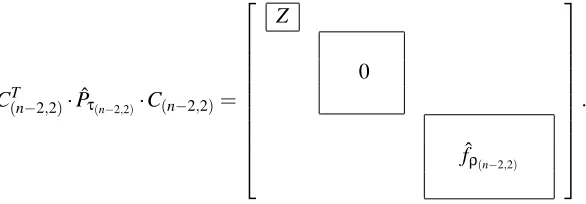
(unordered) “marginals” using Equation 5.
C(nT−2,2)·Pˆτ(n−2,2)·C(n−2,2)=
Z
0
ˆ
fρ(n−2,2) .
The sizes of the irreducible representation matrices are typically much smaller than their corre-sponding permutation representation matrices. In the case ofλ= (1, . . . ,1)for example, dimτλ=n!
while dimρλ=1. There is a simple combinatorial algorithm, known as the Hook Formula (Sagan,
2001), for computing the dimension ofρλ. While we do not discuss it, we provide a few
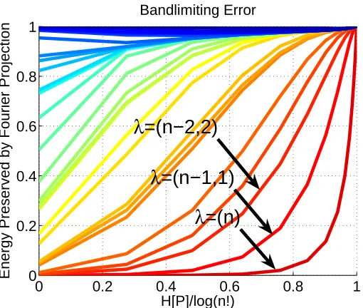
dimen-sionality computations here (Table 3) to facilitate a dicussion of complexity later. Despite providing polynomial sized function approximations, the Fourier coefficient matrices can grow quite fast, and roughly, one would need O(n2k)storage to maintain kth order marginals. For example, we would need to store O(n8) elements to maintain fourth-order marginals. It is worth noting that since the Fourier transform is invertible, there must be n! Fourier coefficients in total, and so∑ρdρ2=|G|=n!.
See Figure 3(b) for an example of what the matrices of a complete Fourier transform on S6would
look like.
In practice, since the irreducible representation matrices are determined only up to equivalence, it is necessary to choose a basis for the irreducible representations in order to explicitly construct the representation matrices. As in Kondor et al. (2007), we use the Gel’fand-Tsetlin basis which has several attractive properties, two advantages being that the matrices are real-valued and orthogonal. See Appendix B for details on constructing irreducible matrix representations with respect to the Gel’fand-Tsetlin basis.
6. Inference in the Fourier Domain
using our compact summaries. One of the main advantages of viewing marginals as Fourier coeffi-cients is that it provides a natural principle for formulating polynomial time approximate inference algorithms, which is to rewrite all inference related operations with respect to the Fourier domain, then to perform the Fourier domain operations ignoring high-order terms.
The idea of bandlimiting a distribution is ultimately moot, however, if it becomes necessary to transform back to the primal domain each time an inference operation is called. Naively, the Fourier Transform on Snscales as O((n!)2), and even the fastest Fast Fourier Transforms for functions on Sn are no faster than O(n2·n!)(see Maslen 1998 for example). To resolve this issue, we present a formulation of inference which operates solely in the Fourier domain, allowing us to avoid a costly transform. We begin by discussing exact inference in the Fourier domain, which is no more tractable than the original problem because there are n! Fourier coefficients, but it will allow us to discuss the bandlimiting approximation in the next section. There are two operations to consider: predic-tion/rollup, and conditioning. While we have motivated both of these operations in the familiar context of hidden Markov models, they are fundamental and appear in many other settings. The assumption for the rest of this section is that the Fourier transforms of the transition and observation models are known. We discuss methods for obtaining the models in Section 8. The main results of this section (excluding the discussions about complexity) extend naturally to other finite groups besides Sn.
6.1 Fourier Prediction/Rollup
We will consider one particular class of transition models—that of random walks over a group, which assumes thatσ(t+1)is generated fromσ(t)by drawing a random permutationπ(t)from some distribution Q(t)and settingσ(t+1)=π(t)σ(t).7 In our identity management example,π(t)represents
a random identity permutation that might occur among tracks when they get close to each other (what we call a mixing event). For example, Q(1,2) =1/2 means that Tracks 1 and 2 swapped identities with probability 1/2. The random walk model also appears in many other applications such as modeling card shuffles (Diaconis, 1988).
The motivation behind the random walk transition model is that it allows us to write the pre-diction/rollup operation as a convolution of distributions on a group. The extension of the familiar notion of convolution to groups simply replaces additions and subtractions by analogous group op-erations (function composition and inverse, respectively):
Definition 7 Let Q and P be probability distributions on a group G. Define the convolution8 of Q and P to be the function[Q∗P] (σ1) =∑σ2Q(σ1σ−1
2 )P(σ2).
Using Definition 7, we see that the prediction/rollup step can be written as:
P(σ(t+1)) =
∑
σ(t)
P(σ(t+1)|σ(t))·P(σ(t)),
=
∑
{(σ(t),π(t)):σ(t+1)=π(t)·σ(t)}
Q(t)(π(t))·P(σ(t)),
7. We placeπon the left side of the multiplication because we want it to permute tracks and not identities. Had we definedπto map from tracks to identities (instead of identities to tracks), thenπwould be multiplied from the right. Besides left versus right multiplication, there are no differences between the two conventions.
8. Note that this definition of convolution on groups is strictly a generalization of convolution of functions on the real line, and is a non-commutative operation for non-Abelian groups. Thus the distribution P∗Q is not necessarily the
(Right-multiplying both sides ofσ(t+1)=π(t)σ(t)
by(σ(t))−1, we see thatπ(t)can be replaced byσ(t+1)(σ(t))−1),
=
∑
σ(t)
Q(t)(σ(t+1)·(σ(t))−1)·P(σ(t)), =hQ(t)∗P
i
(σ(t+1)).
As with Fourier transforms on the real line, the Fourier coefficients of the convolution of distribu-tions P and Q on groups can be obtained from the Fourier coefficients of P and Q individually, using the convolution theorem (see also Diaconis 1988):
Proposition 8 (Convolution Theorem) Let Q and P be probability distributions on a group G. For
any representationρ, h
[
Q∗P i
ρ=Qbρ·Pbρ,
where the operation on the right side is matrix multiplication.
Therefore, assuming that the Fourier transformsPbρ(t)andQb(tρ)are given, the prediction/rollup update rule is simply:
b
Pρ(t+1)←Qb(t)ρ ·Pbρ(t).
Note that the update only requires knowledge of ˆP and does not require P. Furthermore, the update
is pointwise in the Fourier domain in the sense that the coefficients at the representation ρaffect
b
Pρ(t+1)only atρ. Consequently, prediction/rollup updates in the Fourier domain never increase the
representational complexity. For example, if we maintain third-order marginals, then a single step of prediction/rollup called at time t returns the exact third-order marginals at time t+1, and nothing more.
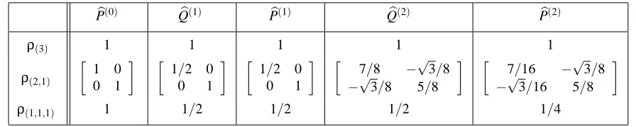
Example 8 We run the prediction/rollup routines on the first two time steps of the example in
Figure 2, first in the primal domain, then in the Fourier domain. At each mixing event, two tracks, i and j, swap identities with some probability. Using a mixing model given by:
Q(π) =
3/4 ifπ=ε
1/4 ifπ= (i,j)
0 otherwise
,
we obtain results shown in Tables 4 and 5.
6.1.1 COMPLEXITY OFPREDICTION/ROLLUP
We will discuss complexity in terms of the dimension of the largest maintained irreducible Fourier
coefficient matrix, which we will denote by dmax (see Table 3 for irreducible dimensions). If
we maintain 2nd order marginals, for example, then dmax =O(n2), and if we maintain 3rd order
marginals, then dmax=O(n3).
σ P(0) Q(1) P(1) Q(2) P(2)
ε 1 3/4 3/4 3/4 9/16
(1,2) 0 1/4 1/4 0 3/16
(2,3) 0 0 0 0 0
(1,3) 0 0 0 1/4 3/16
(1,2,3) 0 0 0 0 1/16
(1,3,2) 0 0 0 0 0
Table 4: Primal domain prediction/rollup example.
b
P(0) Qb(1) Pb(1) Qb(2) Pb(2)
ρ(3) 1 1 1 1 1
ρ(2,1)
1 0
0 1
1/2 0
0 1
1/2 0
0 1
7/8 −√3/8 −√3/8 5/8
7/16 −√3/8 −√3/16 5/8
ρ(1,1,1) 1 1/2 1/2 1/2 1/4
Table 5: Fourier domain prediction/rollup example.
In certain situations, faster updates can be achieved. For example, in the pairwise mixing model of Example 8, the Fourier transform of Q distribution takes the form: ˆQρλ=αIdλ+βρλ(i,j), where
Idλ is the dλ×dλ identity matrix (see also Section 8). As it turns out, the matrixρλ(i,j) can be
factored into a product of O(n)sparse matrices each with at most O(dλ)nonzero entries. To see why, recall the elementary fact that the transposition(i,j)factors into a sequence of O(n)adjacent transpositions:
(i,j) = (i,i+1)(i+1,i+2)···(j−1,j)(j−2,j−1)·(i+1,i+2)(i,i+1).
If we use the Gel’fand-Tsetlin basis adapted to the subgroup chain S1⊂ ···Sn (see Appendix B),
then we also know that the irreducible representation matrices evaluated at adjacent transpositions are sparse with no more than O(dmax2 )nonzero entries. Thus by carefully exploiting sparsity during the prediction/rollup algorithm, one can achieve an O(nd2
max)update, which is faster than O(dmax3 )
as long as one uses more than first-order terms.
6.1.2 LIMITATIONS OF RANDOMWALKMODELS
obser-vations.9 Shin et al. (2005) show that the entropy must increase for a certain kind of random walk on Sn(whereπcould be either the identity or the transposition(i,j)), but in fact, the result is easily
generalized for any random walk mixing model and for any finite group.
Proposition 9
H h
P(t+1)(σ(t+1))i≥maxnHhQ(t)(τ(t))i,HhP(t)(σ(t))io,
where H[P(σ)]denotes the statistical entropy functional, H[P(σ)] =−∑σ∈GP(σ)log P(σ).
Proof We have:
P(t+1)(σ(t+1)) =hQ(t)∗P(t)i(σ(t+1))
=
∑
σ(t)
Q(σ(t+1)·(σ(t))−1)P(t)(σ(t))
Applying the Jensen Inequality to the entropy function (which is concave) yields:
H h
P(t+1)(σ(t+1))i≥
∑
σ(t)
P(t)(σ(t))H h
Q(t)(σ·(σ(t))−1)i, (Jensen’s inequality)
=
∑
σ(t)
P(t)(σ(t))H h
Q(t)(σ)i, (translation invariance of entropy)
=HhQ(t)(σ)i, (since∑σ(t)P(t)(σ(t)) =1).
The proof that HP(t+1)(σ(t+1))≥HP(t)(σ(t))is similar with the exception that we must rewrite
the convolution so that the sum ranges overτ(t).
P(t+1)(σ(t+1)) =hQ(t)∗P(t)i(σ(t+1)),
=
∑
τ(t)
Q(t)(τ(t))P(t)((τ(t))−1·σ(t+1)).
Example 9 This example is based on one from Diaconis (1988). Consider a deck of cards numbered
{1, . . . ,n}. Choose a random permutation of cards by first picking two cards independently, and swapping (a card might be swapped with itself), yielding the following probability distribution over Sn:
Q(π) =
1
n ifπ=ε
2
n2 ifπis a transposition
0 otherwise
. (7)
2 4 6 8 10 12 14 0
0.1 0.2 0.3 0.4 0.5 0.6 0.7 0.8 0.9 1
Entropy with respect to number of shuffles
# shuffles
H/log(n!)
n=3 n=4 n=5 n=6 n=7 n=8
Figure 4: We start with a deck of cards in sorted order, and perform fifteen consecutive shuffles according to the rule given in Equation 7. The plot shows the entropy of the distribu-tion over permutadistribu-tions with respect to the number of shuffles for n=3,4, . . . ,8. When
H(P)/log(n!) =1, the distribution has become uniform.
Repeating the above process for generating random permutationsπgives a transition model for a hidden Markov model over the symmetric group. We can also see (Figure 4) that the entropy of the deck increases monotonically with each shuffle, and that repeated shuffles with Q(π)eventually bring the deck to the uniform distribution.
6.2 Fourier Conditioning
In contrast with the prediction/rollup operation, conditioning can potentially increase the repre-sentational complexity. As an example, suppose that we know the following first-order marginal probabilities:
P(Alice is at Track 1 or Track 2) =.9,and
P(Bob is at Track 1 or Track 2) =.9.
If we then make the following first-order observation: