R E S E A R C H
Open Access
Using information theoretic distance measures
for solving the permutation problem of blind
source separation of speech signals
Eugen Hoffmann
*, Dorothea Kolossa, Bert-Uwe Köhler and Reinhold Orglmeister
Abstract
The problem of blind source separation (BSS) of convolved acoustic signals is of great interest for many classes of applications. Due to the convolutive mixing process, the source separation is performed in the frequency domain, using independent component analysis (ICA). However, frequency domain BSS involves several major problems that must be solved. One of these is the permutation problem. The permutation ambiguity of ICA needs to be resolved so that each separated signal contains the frequency components of only one source signal. This article presents a class of methods for solving the permutation problem based on information theoretic distance measures. The proposed algorithms have been tested on different real-room speech mixtures with different reverberation times in conjunction with different ICA algorithms.
Keywords:blind source separation, independent component analysis, permutation problem
1 Introduction
Blind source separation (BSS) is a technique of recovering the source signals using only observed mixtures when both the mixing process and the sources are unknown. Due to a large number of applications for example in med-ical and speech signal processing, BSS has gained great attention. This article considers the case of BSS for acous-tic signals observed in a real environment, i.e., convolutive mixtures, focusing on speech signals in particular. In recent years, the problem has been widely studied and a number of different approaches have been proposed [1,2]. Many state-of-the-art unmixing methods of acoustic sig-nals are based on independent component analysis (ICA) in the frequency domain, where the convolutions of the source signals with the room impulse response are reduced to multiplications with the corresponding transfer functions. So for each frequency bin, an individual instan-taneous ICA problem arises [2].
Due to the nature of ICA algorithms, obtaining a consis-tent ordering of the recovered signals is highly unlikely. In case of frequency domain source separation, this means that the ordering of outputs may change for each
frequency bin. In order to correctly estimate source signals in the time domain, all separated frequency bins need to be put in a consistent order. This problem is also known as the permutation problem.
There exist several classes of algorithms giving a solu-tion for the permutasolu-tion problem. Approaches presented in [3-6] try to find permutations by considering the cross statistics (such as cross correlation or cross cumulants etc.) of the spectral envelopes of adjacent frequency bins. In [7] algorithms were proposed, that make use of the spectral distance between neighboring bins and try to make the impulse response of the mixing filters short, which corresponds to smooth transfer functions of the mixing system in the frequency domain. The algorithm proposed by Kamata et al. [8] solves the problem using the continuity in power between adjacent frequency com-ponents of the same source. A similar method was pre-sented by Pham et al. [9]. Baumann et al. [10] proposed a solution by comparing the directivity patterns resulting from the estimated demixing matrix in each frequency bin. Similar algorithms were presented in [11-13]. In [14] it was suggested to use the direction of arrival (DOA) of source signals, determined from the estimated mixing matrices, for the problem solution. The approach in [15] is to exploit the continuity of the frequency response of
* Correspondence: [email protected]
Berlin Institute of Technology, Chair of Electronics and Medical Signal Processing, Einsteinufer 17, 10587 Berlin, Germany
the mixing filter. A similar approach was presented in [16] using the minimum of theL1-norm of the resulting
mixing filter and in [17] using the minimum distance between the adjacent filter coefficients. In [18] the authors suggest to use the cosine between the demixing coefficients of different frequencies as a cost function for the problem solution. Sawada et al. [19] proposed an approach based on basis vector clustering of the normal-ized estimated mixing matrices. In [20] a hybrid approach combines spectral continuity, temporal envelope and beamforming alignment with a psychoacoustic post-filter, and in [21] the permutation problem was solved using a maximum-likelihood-ratio between the adjacent fre-quency bins.
However with growing number of the independent components, the complexity of the solution grows. This is true not only because of the factorial increase of per-mutations to be considered, but also because of the degradation of the ICA performance. So not all of the approaches mentioned above perform equally well for an increasing number of sources.
The goal of this article is to investigate the usefulness of information theoretic distance measures for the solution of the permutation ambiguity problem. For this purpose it is assumed that the amplitudes of the estimated indepen-dent signals possess a Rayleigh distribution [22] and the logarithms of the amplitudes possess a generalized Gaus-sian distribution (GGD). It should be noted that the approach in [23] is based on a similar assumption, namely that the extracted signals are generalized Gaussian distrib-uted. The authors handle the problem by comparing the parameters of the GGD of each frequency bin. However the resulting algorithm solves the permutation problem only partially and requires a combination with another approach, for instance [24].aIn contrast, the algorithms proposed in this article deal with the problem in a self-contained way and require no completion by other approaches.
The resulting approaches will be tested on different speech mixtures recorded in real environments with differ-ent reverberation times in combination with differdiffer-ent ICA algorithms, such as JADE [25], INFOMAX [4,26], and FastICA [27,28].
2 Problem formulation
This section provides an introduction into the problem of blind separation of acoustic signals.
At first a general situation will be considered. In a reverberant (real) room,Nacoustic signalss(t) = [s1(t),... sN(t)] are simultaneously active (trepresents the time index). The vector of the source signalss(t) is recorded
with M microphones placed in the room, so that an
observation vectorx(t) = [x1(t), ...xM(t)] results. Due to
the time delay and to the signal reflections, the resulting mixturex(t) is a result of a convolution of the source sig-nal s(t) with an unknown filter tensor a= (a1. . .aK)
whereakis thek-th (kÎ[1...K])M×Nmatrix with filter
coefficients andKis the filter length. This problem can be summarized by
x(t) =
K−1
k=0
ak+1s(t−k) +n(t). (1)
The termn(t) denotes the additive sensor noise. Now the problem is to find a filter matrixw= (w1· · ·wK)so that by applying it to the observation vector x(t), the source signals can be estimated via
y(t) =
K−1
k=0
wk+1x(t−k). (2)
In other words, for the estimated vectory(t) and the source vectors(t),y(t)≈s(t) should hold.
This problem is also known as cocktail-party-problem. A common way to deal with the problem is to reduce it to a set of instantaneous separation problems, for which efficient approaches exist.
For this purpose, the time-domain observation vectors x(t) are transformed into a frequency domain time series by means of the short time Fourier transform (STFT)
X(,τ) =
∞
t=−∞
x(t)w(t−τR)e−jt, (3) where Ω is the angular frequency, τ represents the frame index, and w(t) is a window function (e.g., Han-ning window) of length NFFT, τ represents the frame
index and corresponds to the time shift of he window and Ris the shift size, in samples, between successive windows [29]. Transforming Equation (1) into the fre-quency domain reduces the convolutions to multiplica-tions with the corresponding transfer funcmultiplica-tions, so that for each frequency bin an individual instantaneous ICA problem
X(,τ)≈A()S(,τ) +N(,τ) (4)
arises. A(Ω) is the mixing matrix in the frequency domain,S(Ω,τ) = [S1(Ω,τ), ...,SN (Ω, τ)] represents the
source signals, X(Ω, τ) = [X1(Ω, τ), ..., XM (Ω, τ)],
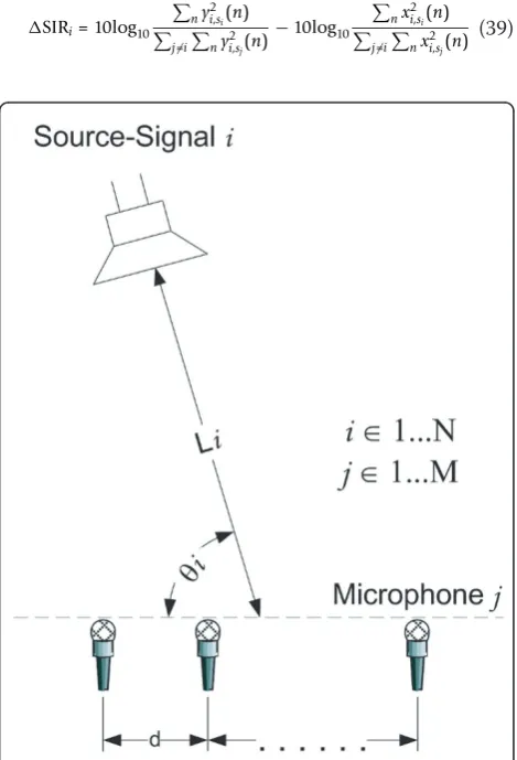
denotes the observed signals, and N(Ω, τ) is the fre-quency domain representation of the additive sensor noise. In order to reconstruct the source signals unmix-ing matrixW(Ω)≈P-1(Ω)A-1(Ω) is derived using com-plex-valued ICA, so that
ˆ
holds. Here Ŷ(Ω, τ) = [Ŷ1(Ω, τ), ..., ŶN(Ω, τ)] is the
time frequency representation of the permutated ICA outputs. In order to solve the permutation problem a correction matrixP(Ω) for each frequency bin has to be found, which is the main topic of this article. The data flow of the whole application is shown in Figure 1.
3 Permutation correction
This section gives an overview over the applied permu-tation correction methods. To resolve the permupermu-tations, the probability density functions (pdfs) of the magni-tudes or of the logarithms of the magnimagni-tudes of the resulting frequency bins are compared. At this point, the assumption is made that adjacent frequency bins of the same source signal possess similar distributions.
3.1 Speech density modeling
3.1.1 Distribution of the speech magnitudes
As shown in [22], for speech signals the distribution of the magnitudes of spectral components can be described by the Rayleigh distribution. The pdf of the Rayleigh dis-tribution of a random variablexis given by
f(x|σ) = x
σ2exp
− x2
2σ2
, (6)
wheresis a shape parameter that can be estimated e. g., by using the maximum likelihood estimator [30].
For the vector of random variablesx = (x1, x2,...xN),
the multivariate Rayleigh distribution can be written as follows
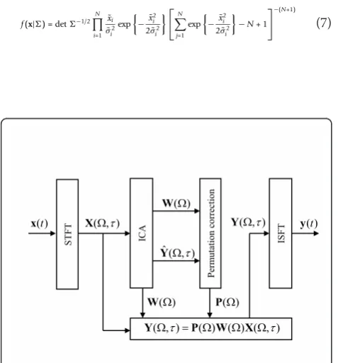
f(x|) = det−1/2 N
i=1
˜ xi ˜ σ2
i
exp
−˜x2i
2σ˜2 i
⎡ ⎣N
j=1
exp
−x˜2i
2σ˜2 i
−N+ 1 ⎤ ⎦
−(N+1) (7)
where
= (x−μ)T(x−μ) (8)
is the symmetric positive definite covariance matrix of x,
˜
x=−1/2(x−μ) (9)
is a vector of the decorrelated random variables andσ˜i
is the shape parameter for the signalx˜i[31][32].b
3.1.2 Distribution of the logarithms of the speech magnitudes
For the approximation of the logarithms of the speech magnitudes the GGD is applied. The PDF of the GGD of a random variablexis given by
f(x|μ,σ,β) = β
2a(1/β)exp
−x−μ
a
β
, (10)
where μ is the mathematical expectation of x. The scale parameterais obtained by
a=σ
(1/β)
(3/β), (11)
and the Gamma function is given by
(z) =
∞
0
uz−1e−udu. (12)
The b-parameter describes the distribution shape and sis the standard deviation of x. However, the b -para-meter is unknown and needs to be estimated e.g., by using the maximum likelihood estimator [33] or the moment estimator [34,35].
For the vector of random variablesx = (x1, x2,...xN),
the multivariate generalized Gaussian PDF can be writ-ten as follows
f(x|μ,,β1. . . βN) = det−1/2 N
i=1
βi
2ai(1/βi)
exp
−˜xi
ai βi
, (13)
whereΣis the covariance matrix ofxand x˜ is a vector of the decorrelated random variables (Equation (9)) [33].
3.2 Distance measures
Suppose the pdfs of magnitudes in two adjacent fre-quency bins
fY(ˆ k,τ)
=
fYˆ1(k,τ)
,. . .,fYˆN(k,τ)
(14)
and
fYˆ(k+1,τ)
=fYˆ1(k+1,τ)
,. . .,fYˆN(k+1,τ)
of separated speech signals Ŷ(Ω, τ) are known. To solve the permutation ambiguity problem, it is necessary to define a pairwise similarity measured(·, ·) between two PDFs, so the overall dependence (distance) results in
DfYˆP(k,τ)
,fYˆ(k+1,τ)
= N
n=1 dfYˆP
n(k,τ)
,fYˆN(k+1,τ)
, (16)
wherekÎ[1, NFFT- 1] is the frequency index,
ˆ
YP(k,τ) =π
ˆ Y(k,τ)
(17)
is a permutation of Ŷ(Ωk, τ), π(x) defines a permuta-tion of the components of the vector x and Nis the
number of separated signals. The total distance D
between a permutated vector of frequency bins,ŶP(Ωk,
τ), and a reference vector in bink + 1, is a sum of dis-tances between each pairYˆnP(k,τ)andŶn(Ωk+1,τ).
Below, several information theoretic similarity mea-sures will be considered, which seem to be suitable for the solution of the permutation ambiguity problem. But first a definition of entropy or “self-information” is necessary.
The generalized formulation of entropy was given by Rényi and is known as the Rényi entropy in information theory [36,37]. The Rényi differential entropy of order a, where a ≥ 0, for a random variable with a pdff(x) whose support is a setX, is defined as
Hα(f(x)) = 1 1−αlog
⎛
⎝
X
fα(x)dx
⎞
⎠. (18)
It can be shown, that in limit fora®1,Ha(f(x))
con-verges to the Shannon entropy [37,38],
H1(f(x)) =−
X
f(x) logf(x)dx. (19)
Similarly to the marginal entropy above, the joint entropy of a vector of random variablesx = (x1,x2, ..., xN) is defined as
Hα(f(x)) = 1 1−αlog
⎛
⎝
X
fα(x)dx
⎞
⎠, (20)
wheref(x) is the multivariate pdf.
At this point it is possible to introduce the necessary dependence measures that will be used as the pairwise similarity measured(·, ·) in Equation (16):
- Rényi generalized divergencebetween two distri-butionsf(x) andg(x) of ordera, where a≥0, is defined [36] as
dα(f(x)||g(x)) = 1
α−1log
fα(x)g1−α(x)dx
. (21)
Special cases of Equation (21) [39] are the - Bhattacharyya coefficient
d1/2(f(x)||g(x)) =−2 log f(x)g(x)dx
, (22)
- Kullback-Leibler divergence
d1(f(x)||g(x)) =
f(x) logf(x)
g(x)dx, (23)
- Log distance
d2(f(x)||g(x)) = logE
f(x) g(x)
, (24)
where E[·] denotes the statistical expectation accord-ing tof(x),
- and log of the maximum ratio
d∞(f(x)||g(x)) = log sup
x
f(x)
g(x). (25)
Rényi’s divergence describes the alikeness between two distributions. The smaller the Rényi divergence, the more similar the distributions are. The main advantage of the Rényi divergence is the small computational bur-den. The problem in using the Rényi divergence is the fact that this measure is not symmetric, so typicallyda(f
(x)||g(x))≠da(g(x)||f(x)), and not bounded, so infinite
values can arise.
-Mutual informationfor a vector of random variables X = (X1,X2, ...,XK) is defined as the Kullback-Leibler
divergence between the product of the distribution func-tionsKi=1fXi(xi)and the multivariate distributionfx(x)
I(X) =d1
fx(x)
K
i=1 fXi(xi)
!
(26)
=
fx(x) log
fX(x)
K
i=1fXi(xi)
dX (27)
=
fx(x) logfx(x)dx−
fX(x) log
K
i=1
fXi(xi)dx (28)
=
K
i=1
H1(fXi(xi))−H1(fx(x)) (29)
whereH1(fXi(xi))is the marginal entropy andH1(fx(x))
Mutual information gives the amount of information contained in the random variables ofX. Since for the computation of the term fx(x) is taken into account i.e., the dependencies are considered, the mutual informa-tion is a stronger cost funcinforma-tion than Rényi divergence and using it for resolving the permutations, better results are to be expected.
- The Jensen-Rényi divergenceof the vector of ran-dom variables X= (X1,X2, ...,XK) of ordera, wherea≥
0, is defined [40] as
dJRα(X) =Hα
1 K
K
i=1 fXi(xi)
!
− 1
K
K
i=1
Hα(fXi(x)). (30)
The Jensen-Rényi divergence is based on the Kullback-Leibler divergence and can be seen as an extension of it with the difference that it is symmetricc and always of finite value. On the other hand, due to the fact that the distributions of the random variables are compared indirectly using the average 1
K
"K
i=1fXi(x), the
Jensen-Rényi divergence can be seen as an alternative to the mutual information [41]. In fact, as shown in [42], both measures show similar characteristics.
- The modified Jensen-Rényi divergence. The Jen-sen-Rényi-divergence from the Equation (30) measures the distance between two distributionsfX(x) and fY(x) in respect to a third point in the distribution space. In this case, the third point is chosen as the average of the two distributions. This approach is justified because of the concavity of the entropy in distribution space
Hα
fX(x) +fY(x)
2
≥ Hα(fX(x)) +Hα(fY(x))
2 . (31)
In principle, it is possible to define the distance in respect to any other point, if the assumption of the con-cavity for this point holds. Such a point can be chosen as an average over the random variables, the distribu-tions of which are currently analyzed.
For the entropy of a random variableX
Hα(fX(x))∝ ||fX(x)||α (32) holds, and for the entropy of the sum of two random variablesXandY[38,43]
Hα(fX+Y(x))∝ ||fX(x)∗fY(x)||α. (33) ||·||a denotes the a norm operator and ٭ stands for convolution. Using the entropy power inequality [38] for the case ofa= 1, and extending Young’s inequality [44] for the case ofa≠1, it can be shown [45], that
Hα(fX+Y(x))≥max(Hα(fX(x)),Hα(fY(x))). (34)
Since
max(a,b)≥ a+b
2 (35)
holds, the inequality in Equation (34) can be rewritten as
Hα(fX+Y(x))≥
Hα(fX(x)) +Hα(fY(x))
2 . (36)
So, at this point a modification of the Jensen-Rényi divergence is proposed. This distance measure of the vector of random variablesX= (X1,X2, ...,XK) of order
a, wherea≥0, is defined as
dmJRα(X) =Hα(fX¯(x))−
1 K
K
i=1
Hα(fXi(x)) (37)
where X¯ = 1K"Ki=1XiIn the way the modified
Jensen-Rényi divergence is used here, this distance measure describes the amount of new information coming to a spectrogram if an adjacent frequency bin Y(Ωk+1, τ) is
included. The lesser the new information provided, the closer the frequency bins are. This modification has less computational burden than the classical Jensen-Rényi divergence, since for Hα(fX˜(x)), only one pdf has to be calculated instead of Kin the Jensen-Rényi divergence. Furthermore, for the entropy Hα(fX¯(x))there exists an analytical solution, which improves the accuracy of the results.
3.3 The Permutation correction algorithm
In this section the actual permutation correction algo-rithm will be discussed. As mentioned before, it will be assumed that subsequent frequency bins of the same source signal possess similar distributions. The similarity between the frequency bins is measured by applying the measures given in Equations (21),(29), (30), and (37) in the optimization of Equation (16).
However, as mentioned in [14] the use of only one frequency bin as a reference bin for the correction causes a risk of a misalignment of the algorithm. To avoid this problem, the approach presented in [5] uses an average value of the already corrected frequency bins. So, the Equation (16) will be redefined as
D
fYˆP(k,τ)
,f
1
L k+1+L
l=k+1 Yˆ(l,τ)
!
=
N
n=1
d
fYˆP n(k,τ)
,f
1
L k+1+L
l=k+1 Ynˆ(l,τ)
! (38)
Algorithm 1
1. Initialization: Start with the frequencydSetk=NFFT/
2.
2. Estimate the parameters of the Rayleigh distribution of |Ŷ(Ωk, τ)| and of the average ofLalready corrected
bins 1
ˆ
L
"Lˆ
l=k+1| ˆYn(l,τ)|, with
ˆ
L= min(k+ 1 +L,NFFT
#
2 + 1)−(k+ 1) using
Equa-tions (6)-(9).
3. CalculateD
f
|ˆYP(k,τ)|
,f
1
ˆ
L
"Lˆ
l=k+1|ˆY(l,τ)|
as defined in Equation (38) for all possible permutations of |Ŷ(Ωk,τ)|.
4. Choose the permutation π+(|Ŷ(Ωk, τ)|) with the
most dependent value ofD.
5. Correct the current frequency bin in order with the best permutationπ+(|Ŷ(Ωk,τ)|).
6. Decrementkand if k≠0 go to Step 2.
The same scheme can be applied on the logarithms of the spectral magnitudes of the signals log |Ŷ(Ωk, τ)| instead of |Ŷ(Ωk, τ)| and using generalized Gaussian instead of Rayleigh distributions. In that case Algorithm 2 results.
Algorithm 2
1. Initialization: Start with the frequencyk=NFFT/2.
2. Estimate the GGD parameters of log |Ŷ(Ωk,τ)| and
of the average of L already corrected bins
log(1ˆ
L
"Lˆ
l=k+1| ˆYn(l,τ)|), with
ˆ
L= min(k+ 1 +L,NFFT
#
2 + 1)−(k+ 1) using
Equa-tions (10)-(13).e
3. Calculate
D
f
log|ˆYP(k,τ)|
,f
log(1ˆ
L
"Lˆ
l=k+1|ˆY(l,τ)|)
as
defined in Equation (38) for all possible permutations of |Ŷ(Ωk,τ)|.
4. Choose the permutationπ+(log |Ŷ(Ωk,τ)|) with the
most dependent value ofD.
5. Correct the current frequency bin in order with the best permutationπ+(log |Ŷ(Ωk,τ)|).
6. Decrementkand if k≠0 go to Step 2.
The Algorithms 1 and 2 will be used in the following sections for the experimental comparison of the distance measures given in Equations (21),(29), (30), and (37).
4 Experiments and results 4.1 Conditions
For the evaluation of the proposed approaches, two dif-ferent sets of recordings were used. In the first data set, different audio files from the TIDigits database [46] were used and mixtures with up to four speakers were recorded under real room conditions. The distance between speakers and the center of a linear microphone array was varied between 0.9 and 2 m. The second
dataset was recorded by Sawada [47]. Here also mixtures with up to four speakers are presented. All of the mix-tures were made with the same number of microphones as the number of speakers in the mixture (M =N), i.e., in each mixture a determined problem is considered so the classical ICA algorithms for source separation can be applied. The experimental setups are presented sche-matically in Figure 2 and the experimental conditions are summarized in Tables 1, 2, 3, and 4.
4.2 Parameter settings
The algorithms were tested on all recordings, which were first transformed to the frequency domain at a resolution ofNFFT= 1, 024. For calculating the
spectro-gram, the signals were divided into overlapping frames with a Hanning window and an overlap of 3/4 ·NFFT.
4.3 ICA performance measurement
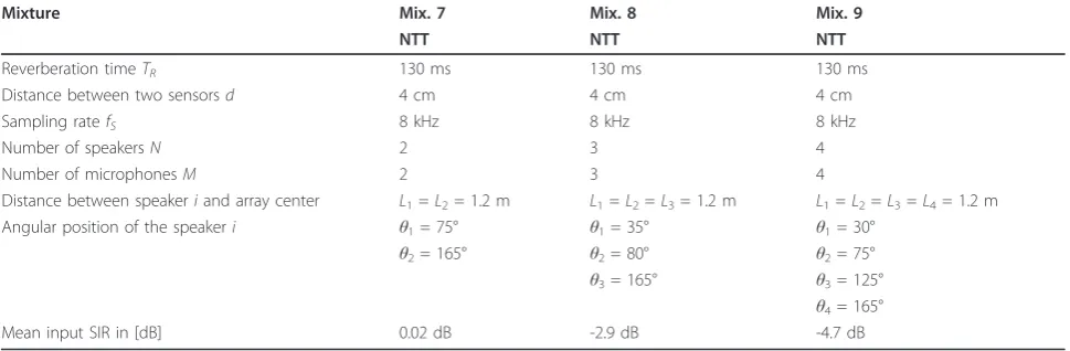
For calculation of the effectiveness of the proposed algo-rithm, the improvementΔSIR of the signal to interfer-ence ratio
SIRi= 10log10
"
ny2i,si(n)
"
j=i
"
ny2i,sj(n)
−10log10
"
nx2i,si(n)
"
j=i
"
nx2i,sj(n) (39)
Figure 2 Experimental Setup. Li is the distance between
speakeriand array center.θiis the angular position of the
was used as a measure of the separation performance and the signal to distortion ratio (SDR)
SDRi= 10log10
"
nx2ksi(n) "
n(xksi(n)−αyisi(n−δ))
2 (40)
as a measure of the signal quality. Hereyi,sjis thei-th
separated signal with only the sourcesjactive, andxk,sjis
the observation obtained by microphone kwhen onlysj
is active. a and δ are parameters for phase and
Table 1 Mixture characteristics
Mixture Mix. 1 Mix. 2 Mix. 3
TU Berlin TU Berlin TU Berlin
Reverberation timeTR 159 ms 159 ms 159 ms
Distance between two sensorsd 3 cm 3 cm 3 cm
Sampling ratefS 11 kHz 11 kHz 11 kHz
Number of speakersN 2 3 4
Number of microphonesM 2 3 4
Distance between speakeriand array center L1=L2= 0.9 m L1=L2=L3= 0.9 m L1=L2=L3=L4= 0.9 m
Angular position of the speakeri θ1= 50° θ1= 30° θ1= 25°
θ2= 115° θ2= 80° θ2= 80°
θ3= 135° θ3= 130° θ4= 155°
Mean input SIR in [dB] -0.1 dB -3 dB -5 dB
Table 2 Mixture characteristics
Mixture Mix. 4 Mix. 5 Mix. 6
TU Berlin TU Berlin TU Berlin
Reverberation timeTR 189 ms 189 ms 189 ms
Distance between two sensorsd 3 cm 3 cm 3 cm
Sampling ratefS 11 kHz 11 kHz 11 kHz
Number of speakersN 2 3 4
Number of microphonesM 2 3 4
Distance between speakeriand array center L1=L2= 2.0 m L1=L2=L3= 2.0 m L1=L2=L3=L4= 2.0 m
Angular position of the speakeri θ1= 75° θ1= 35° θ1= 30°
θ2= 165° θ2= 80° θ2= 75°
θ3= 165° θ3= 125° θ4= 165°
Mean input SIR in [dB] -0.04 dB -3.4 dB -6.9 dB
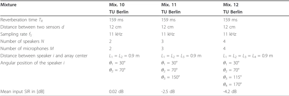
Table 3 Mixture characteristics
Mixture Mix. 7 Mix. 8 Mix. 9
NTT NTT NTT
Reverberation timeTR 130 ms 130 ms 130 ms
Distance between two sensorsd 4 cm 4 cm 4 cm
Sampling ratefS 8 kHz 8 kHz 8 kHz
Number of speakersN 2 3 4
Number of microphonesM 2 3 4
Distance between speakeriand array center L1=L2= 1.2 m L1=L2=L3= 1.2 m L1=L2=L3=L4= 1.2 m
Angular position of the speakeri θ1= 75° θ1= 35° θ1= 30°
θ2= 165° θ2= 80° θ2= 75°
θ3= 165° θ3= 125° θ4= 165°
amplitude chosen to optimally compensate the differ-ence betweenyi,sjand xk,sj[19].
For measuring the performance of the proposed algo-rithms on all speakers present in a mixture recording, an averageΔSIR
SIR = 1 N
N
i=1
SIRi (41)
and SDR
SDR = 1 N
N
i=1
SDRi (42)
were used, whereNis the number of speakers in the considered mixture.
4.4 Experimental results
In this section the experimental results of the signal separation will be compared. All the mixtures from Tables 1, 2, 3, and 4 were separated by JADE, INFO-MAX, and the FastICA algorithm and the permutation problem was solved using either Algorithm 1 or 2 from Section 3.3 and distance measures from Equations (21), (29), (30), and (37). For each result the performance is calculated using Equations (39) and (40).
Figures 3 and 4 show the behavior of three different approaches in terms of ΔSIR and SDR (Equations (41) and (42)) over the mixtures for the Infomax approach.
In Tables 5 and 6, the separation results are averaged for each distance measure for the mixtures of 2, 3, and 4 signals separately. M2 in Tables 5 and 6 contains the
Table 4 Mixture characteristics
Mixture Mix. 10 Mix. 11 Mix. 12
TU Berlin TU Berlin TU Berlin
Reverberation timeTR 159 ms 159 ms 159 ms
Distance between two sensorsd 12 cm 12 cm 12 cm
Sampling ratefS 11 kHz 11 kHz 11 kHz
Number of speakersN 2 3 4
Number of microphonesM 2 3 4
Distance between speakeriand array center L1=L2= 0.9 m L1=L2=L3= 0.9 m L1=L2=L3=L4= 0.9 m
Angular position of the speakeri θ1= 30° θ1= 30° θ1= 30°
θ2= 70° θ2= 70° θ2= 70°
θ3= 150° θ3= 115° θ4= 170°
Mean input SIR in [dB] 0.02 dB -2.5 dB -4.2 dB
1 2 3 4 5 6 7 8 9 10 11 12 0
5 10 15
Mixture #
SIR (dB)
1 2 3 4 5 6 7 8 9 10 11 12 0
2 4 6 8 10 12
Mixture #
SDR (dB)
averageΔSIR/SDR of the separation results of Mix. 1, Mix. 4, Mix. 7 and Mix. 10, cf. Tables 1, 2, 3, and 4. Similarly, M3 contains the separation results of Mix. 2,
Mix. 5, Mix. 8 and Mix. 11, and M4 those of Mix. 3,
Mix. 6, Mix. 9 and Mix. 12.
4.5 Discussion
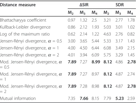
The calculated results show the usefulness of the pro-posed method for permutation correction, though not all of the applied distance measures perform equally. As already mentioned above, the best results were achieved using mutual information and the modified
Jensen-Rényi divergence, while results obtained using general-ized Rényi divergence are rather poor. This is especially the case, if a = 2 is used. Of all the applied distance measures based on the generalized Rényi divergence, the best performance was achieved in the case of the Bhat-tacharyya coefficient, i.e., a = 0.5. A similar tendency can be seen with “classical” Jensen-Rényi divergence. Here the best results were achieved usinga= 1. In con-trast, correction based on mutual information and the modified Jensen-Rényi divergence provides stable good results.
The poor performance in the case of generalized Rényi divergence can be explained by fact that the assumed
1 2 3 4 5 6 7 8 9 10 11 12 0
5 10 15
Mixture #
SIR (dB)
1 2 3 4 5 6 7 8 9 10 11 12 0
2 4 6 8 10 12
Mixture #
SDR (dB)
Figure 4Results obtained by Infomax and Algorithm 2 using‘٭’mutual information witha= 1,‘Δ’Jensen-Rényi divergence witha= 1 and‘ο’modified Jensen-Rényi divergence witha= 1 over the mixtures.
Table 5 Average values of the obtained results of
Algorithm 1 in terms ofΔSIR and SDR for each distance
measure
Distance measure ΔSIR SDR
M2 M3 M4 M2 M3 M4
Bhattacharyya coefficient 0.97 1.32 2.5 3.21 2.77 1.78 Kullback-Leibler divergence 0.86 2.12 1.93 5.03 3.01 1.02 Log of the maximum ratio 0.62 2.14 1.22 4.63 2.76 0.82 Jensen-Rényi divergence,a= 0.5 3.00 3.65 5.44 5.33 3.17 1.43 Jensen-Rényi divergence,a= 1 4.00 4.50 6.44 6.08 3.49 2.15 Jensen-Rényi divergence,a= 2 4.01 3.94 6.09 5.75 3.29 1.45 Mod. Jensen-Rényi divergence,a
= 0.5
7.89 7.27 8.99 8.12 4.86 2.78
Mod. Jensen-Rényi divergence,a = 1
7.89 7.27 8.97 8.12 4.87 2.74
Mod. Jensen-Rényi divergence,a = 2
7.89 7.28 8.98 8.12 4.87 2.78
Mutual information 7.35 7.66 8.15 7.79 5.23 2.59
Mistands for the averageΔSIR/SDR value calculated over all mixtures ofN=i signals (cf. Tables 1, 2, 3, and 4). The best performance for each caseMiis marked in bold.
Table 6 Average values of the obtained results of
Algorithm 2 in terms ofΔSIR and SDR for each distance
measure
Distance measure ΔSIR SDR
M2 M3 M4 M2 M3 M4
Bhattacharyya coefficient 2.21 3.23 3.54 5.53 3.65 1.10 Kullback-Leibler divergence 3.78 5.23 5.47 5.97 4.2 1.46 Log of the maximum ratio 3.52 4.99 4.14 6.32 4.12 1.14 Jensen-Rényi divergence,a= 0.5 3.83 4.93 5.77 6.19 3.92 1.64 Jensen-Rényi divergence,a= 1 4.00 5.04 5.45 6.39 4.12 1.44 Jensen-Rényi divergence,a= 2 2.84 4.42 5.34 6.04 4.14 1.41 Mod. Jensen-Rényi divergence,a
= 0.5
7.31 8.14 8.53 8.01 5.63 2.44
Mod. Jensen-Rényi divergence,a = 1
7.35 8.15 8.61 8.07 5.67 2.47
Mod. Jensen-Rényi divergence,a = 2
7.40 8.27 8.43 8.12 5.76 2.50
Mutual information 7.31 8.50 8.37 8.18 6.00 2.60
models of the probability distribution of the amplitudes and log amplitudes are not exact enough to be used with generalized Rényi divergence for a successful solu-tion of the permutasolu-tion problem. As can be seen in Figure 5, the distribution of the lower frequency bins of a speech signal can be only roughly modeled with Ray-leigh pdf. In contrast the higher frequencies can be seen as Rayleigh distributed variables. This causes a high error rate in the permutation correction at lower fre-quencies, when the generalized Rényi divergence is used. Since, as shown in [48], the lower frequencies play a more significant role in BSS of the speech signals than the higher frequencies, the low values of the SIR and SDR are explainable. The same holds for the distribu-tion of the log amplitudes. This problem can be solved
using a more exact model for the pdf of the speech sig-nals such as Rayleigh mixture models (RMM) for the amplitudes or Gaussian mixture models (GMM) for the log amplitudes and is the subject of the future study.
Furthermore, the effects of the various reverberation times on the performance of different distance measures are going to be studied in the future. While, as it can be seen in Figures 3 and 4, the performance of the separa-tion system decreases with a growing reverberasepara-tion time of the environment, the effect of reverberation time on different methods of permutation correction should be analyzed in a more exact way.
On the other hand, the assumption of the Rayleigh distribution and GGD is good enough for permutation correction with mutual information and the modified
0 0.5 1 1.5 2
0 0.1 0.2 0.3
0.4 a)
Relative frequency
Histogram Rayleigh pdf
0 0.1 0.2 0.3 0.4
0 0.05 0.1 0.15
0.2 b)
Histogram Rayleigh pdf
0 0.01 0.02 0.03
0 0.02 0.04 0.06 0.08 0.1 0.12
c)
Amplitude
Relative frequency
Histogram Rayleigh pdf
0 0.05 0.1 0.15 0.2 0.25
0 0.1 0.2 0.3 0.4 0.5
d)
Amplitude
Histogram Rayleigh pdf
Jensen-Rényi divergence, since these distance measures are not as sensitive to the inter frequency-bin pdf per-turbations as the generalized Rényi divergence. Further-more, in this case there exists an analytical solution for modified Jensen-Rényi divergence, which reduces the computational burden of the algorithm and improves the accuracy of the solution.
As it can be seen in Tables 5 and 6, the separation formance of Algorithm 1 is slightly better than the per-formance of Algorithm 2. A possible explanation for this issue is the fact that for the Rayleigh pdf just one para-meter has to be estimated instead of 2 parapara-meters in case of GGD. Furthermore the estimation of the GGD para-meters is more complicated than the estimation of thes in case of Rayleigh distribution. These might cause the uncertainties and errors in the permutation correction.
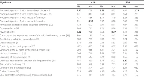
In the next step, the best four of the proposed meth-ods were compared with some other approaches from Section 1. In Table 7, the results of the comparison are shown. As can be seen, the proposed method (Algo-rithm 1 with the modified Jensen-Rényi divergence,a= 2) performs better than other algorithms in terms of ΔSIR in most cases.
5 Conclusions
In this article, a method for the permutation correction in convolutive source separation has been presented. The approach is based on the assumption that magnitudes of
speech signals adhere to a Rayleigh distribution and the logarithms of magnitudes can be modeled by a GGD. The assumption of Rayleigh or GG distributed signals allows to use information theoretic similarity measures. The information theoretic distance measures are used to detect similarities in subsequent frequency bins after bin-wise source separation is completed, in order to group the frequency bins coming from the same source. Beside the existing information theoretic distance measures, a modification of the Jensen-Rényi divergence is proposed. This modified distance measure shows very good results for the considered problem.
The proposed method has been tested on different reverberant speech mixtures in connection with different ICA algorithms. The experimental results and the com-parison with today’s state-of-the-art approaches for per-mutation correction show the usefulness of the proposed method. Further, the experimental results have shown that the method performs best using either the mutual information or the modified Jensen-Rényi diver-gence criterion (Tables 5 and 6). This fact may be explained at least partially by the ability of the Jensen-Renyi divergence and the mutual information to utilize temporal dependence structure, which puts these two criteria ahead of the Rényi generalized divergence and its special cases of the Kullback-Leibler divergence and the log maximum ratio, which we considered as alternatives.
Table 7 Average values of the obtained results in terms ofΔSIR and SDR for each distance measure
Algorithms ΔSIR SDR
M2 M3 M4 M2 M3 M4
Proposed Algorithm 1 with Jensen-Rényi div.,a= 2 7.90 7.28 8.98 8.12 4.87 2.78 Proposed Algorithm 2 with Jensen-Rényi div.,a= 0.5 7.31 8.14 8.53 8.01 5.63 2.44 Proposed Algorithm 1 with mutual information 7.35 7.66 8.15 7.79 5.23 2.59 Proposed Algorithm 2 with mutual information 7.31 8.50 8.37 8.18 6.00 2.60 Permutation correction based on phase difference [50] 7.38 6.77 7.99 8.11 4.87 2.69
Cross-correlation [4] 7.44 7.61 7.76 8.16 5.35 2.63
Power ratio [51] 7.90 7.86 8.53 8.37 5.42 2.68
Continuity of the impulse response of the calculated mixing system [15] 3.93 1.83 2.14 5.67 2.98 0.89
Amplitutde modulation decorrelation [3] 6.89 7.55 8.02 7.83 5.24 2.64
Cross-cumulants [4] 3.10 2.16 2.42 5.53 2.80 0.61
Continuity of the mixing system [17] -0.33 0.65 0.93 4.37 2.52 0.77
Minimum of theL1-norm of the mixing system [16] 0.04 0.65 1.41 3.94 3.32 1.02
p-Norm distance (p= 1) [8] 6.05 7.60 7.68 7.37 5.51 2.38
Clustering of the amplitudes [9] 6.93 5.17 5.22 8.00 4.56 1.77
Likelihood ratio criterion between the frequency bins [21] 7.47 8.33 8.74 8.07 6.17 2.67
Basis vector clustering [19] 7.08 5.40 6.49 7.63 4.32 1.92
Minima of the beampattern [10] 7.40 3.74 2.81 7.74 3.24 0.82
Cosine distance [18] 5.33 4.78 4.56 6.76 4.26 1.74
GGD parameter comparison and cross-correlation [23] 0.45 4.64 6.39 4.13 3.71 1.77
Appendix 1
To calculate the distance measures from Equation (21), (29), (30), and (37), in most cases an integral has to be solved. The Rényi differential entropy (Equation (18)) in case of the Rayleigh distribution is calculated as
Hα(X) = 1 1−αlog
⎛
⎝
X
fXα(x)dx
⎞
⎠ (43)
= log
σ
√ 2
+ 1 1−αlogA+
1 1−αlog
α−α
2+ 1 2
, (44)
wheresis the shape parameter of the Rayleigh distri-bution and
A=α(−α+α2− 1
2). (45)
Settinga® 1 the Equation (44) becomes
H1(x) = 1 + log√α 2+
γ
2, (46)
wheregis the Euler-Mascheroni constant g≈0.57722. For the GG distribution, the entropies can be com-puted as
HRα(X) = 1 1−αlog
⎛
⎝
X
fXα(x)dx
⎞
⎠ (47)
= 1 1−α logα
−1/βX−log
βX
2a(1$βX)
!
(48)
and
H1(X) = 1
βX −
log
βX
2a(1$βX)
!
. (49)
The solution of the Equation (46) is given in [38]. The solutions of the Equations (44) and (48) were derived using MATHEMATICA. For the distance measures without an analytical solution the trapezoidal rule for numerical integration was applied [49].
Appendix 2
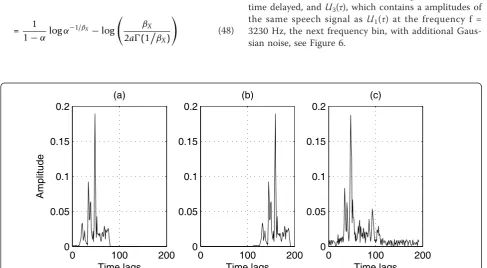
Since information theoretic similarity measures make use only of the pdfs of the signals, a question may arise, as to whether temporal dependence structures of the signals are utilized at all in the suggested framework. The temporal structure is taken into account indirectly in the applied similarity measures, since each of the measures contains a term where either the joint prob-ability, the pdf of the mean value of the random vari-ables (Equation (37)), the mean of the pdf or a quotient of the pdfs is considered. These are the terms where the values of the distribution functions produced at the same time domain window are“compared”.
To demonstrate this issue, the following example was constructed: We compare signalU1(τ), which contains
amplitudes of a speech signal at the frequency f = 3219.2 Hz, U2(τ) which is the same signal asU1(τ) but
time delayed, andU3(τ), which contains a amplitudes of
the same speech signal as U1(τ) at the frequency f =
3230 Hz, the next frequency bin, with additional Gaus-sian noise, see Figure 6.
0 100 200
0 0.05 0.1 0.15 0.2
Time lags
Amplitude
(a)
0 100 200
0 0.05 0.1 0.15 0.2
Time lags (b)
0 100 200
0 0.05 0.1 0.15 0.2
Time lags (c)
Figure 6Constructed signals for demonstration. (a) SignalU1(τ) is a speech signal at the frequencyf= 3, 219.2 Hz, (b)U2(τ) is the same
signal asU1(τ) but time delayed and (c) signalU3(τ) contains amplitudes of the same speech signal asU1(τ) at the frequencyf= 3, 230 Hz (the
For each signal pair 〈U1(τ), U2(τ)〉,〈U1(τ), U3(τ)〉, 〈log
(U1(τ)), log(U2(τ))〉and〈log(U1(τ)), log(U3(τ))〉, the
simi-larity measures from Equations (21), (29), (30), and (37) were applied. The results of the signal comparison can be found in Tables 8 and 9.
As can be seen, for this example each similarity measure that was considered in this article ratesU1(τ) more similar
toU3(τ) than toU2(τ),fwhich implies that the temporal
dependencies and correlations were not ignored during the computation of the probability distribution functions.
In contrast to the other measures, in the case of the Rényi generalized divergence defined in Equation (21), and in its special cases of the Kullback-Leibler diver-gence and the log maximum ratio, the time dependency can not be taken into account in this manner. Still, these similarity measures can also be used for permuta-tion correcpermuta-tion, since the situapermuta-tion we considered in the example above is rather artificial and cannot be expected for realistic situations with two speech signals as the desired sources.
Endnotes a
In the cases where no permutation correction by the means of the comparison of the GGD parameters is
possible, the problem is handled by applying the correla-tion based permutacorrela-tion correccorrela-tion approach.bEquation (7) is a special case of the multivariate Weibull distribu-tion with a = 1 and ci = 2 [32, Equation (14)]. cE.g.
dJRα(X1,X2) =dJRα(X2,X1). dThe proposed algorithm
solves the permutations problem starting with the higher frequency bins. The first frequency bin in this case is the bin with k =NFFT/2 + 1. Since there is no
other definition of the correct order of the signals, the signal order in frequency bin k = NFFT/2+1 will be
assumed as correct.eFor the experiments from the Sec-tion 4 the parameterbwas calculated using the approxi-mation for the inverse function as proposed in [34].
f
The more dependent the signals are, the higher the value of the mutual information Equation (29) becomes, while simultaneously, the values of the similarity mea-sures from (21), (30), and (37) decrease.
Competing interests
The authors declare that they have no competing interests.
Received: 31 October 2011 Accepted: 3 April 2012 Published: 3 April 2012
Table 8 Comparison of signal pairs〈U1(τ),U2(τ)〉and〈U1(τ),U3(τ)〉with each distance measure
Distance measure 〈U1(τ),U2(τ)〉 〈U1(τ),U3(τ)〉
Bhattacharyya coefficient 0,09 0,59
Kullback-Leibler divergence 0,00 0,16
Log of the maximum ratio 0,00 0,16
Jensen-Rényi divergence witha= 0.5 0,43 0,23
Jensen-Rényi divergence witha= 1 1,92 0,22
Jensen-Rényi divergence witha= 2 68,35 45,4
Modified Jensen-Rényi divergence witha= 0.5 0,12 0,02
Modified Jensen-Rényi divergence witha= 1 0,35 0,04
Modified Jensen-Rényi divergence witha= 2 31,06 2,50
Mutual information 15,53 16,46
The most dependent value of each distance measure is marked in bold.
Table 9 Comparison of signal pairs〈log(U1(τ)), log(U2(τ))〉and〈log(U1(τ)), log(U3(τ))〉with each distance measure
Distance measure 〈log(U1(τ)), log(U2(τ))〉 〈log(U1(τ)), log(U3(τ))〉
Bhattacharyya coefficient 0,03 0,71
Kullback-Leibler divergence 0,0 0,03
Log of the maximum ratio 0,0 0,30
Jensen-Rényi divergence,a= 0.5 17,83 7,48
Jensen-Rényi divergence,a= 1 7,54 1,58
Jensen-Rényi divergence,a= 2 0,99 0,01
Mod. Jensen-Rényi divergence,a= 0.5 4,79 1,26
Mod. Jensen-Rényi divergence,a= 1 1,23 0,26
Mod. Jensen-Rényi divergence,a= 2 0,11 0,01
Mutual information 4,59 6,43
References
1. A Mansour, M Kawamoto, ICA papers classified according to their applications and performances. IEICA Trans. Fundam.E86-A(3), 620–633 (2003)
2. MS Pedersen, J Larsen, U Kjems, LC Parra, Convolutive blind source separation methods,Springer Handbook of Speech Processing and Speech Communication, Springer Verlag, Berlin/Heidelberg, pp. 1065–1094 (2008) 3. J Anemüller, B Kollmeier, Amplitude modulation decorrelation for convolutive
blind source separation, inProc. ICA 2000, Helsinki, pp. 215–220 (2000) 4. C Mejuto, A Dapena, L Castedo, Frequency-domain infomax for blind
separation of convolutive mixtures, inProc. ICA 2000, Helsinki, pp. 315–320 (2000)
5. N Murata, S Ikeda, A Ziehe, An approach to blind source separation based on temporal structure of speech signals. Neurocomputing.41(1-4), 1–24 (2001) 6. VG Reju, SN Koh, IY Soon, Partial separation method for solving
permutation problem in frequency domain blind source separation of speech signals. Neurocomputing.71, 2098–2112 (2008)
7. L Parra, C Spence, B De Vries, Convolutive blind source separation based on multiple decorrelation, inProc. IEEE NNSP Workshop, (Cambridge, UK, 1998), pp. 23–32
8. K Kamata, X Hu, H Kobatake, A new approach to the permutation problem in frequency domain blind source separation, inProc. ICA 2004, Granada, Spain, pp. 849–856 (Sept 2004)
9. D-T Pham, C Servière, H Boumaraf, Blind separation of speech mixtures based on nonstationarity, inIEEE Signal Processing and Its Applications, Proceedings of the Seventh International Symposium, pp. 73–76 (2003) 10. W Baumann, D Kolossa, R Orglmeister, Maximum likelihood permutation
correction for convolutive source separation, inICA 2003, pp. 373–378 (2003)
11. S Kurita, H Saruwatari, S Kajita, K Takeda, F Itakura, Evaluation of frequency-domain blind signal separation using directivity pattern under reverberant conditions, inICASSP2000, pp. 3140–3143 (2000)
12. M Ikram, D Morgan, A beamforming approach to permutation alignment for multichannel frequency-domain blind speech separation, inICASSP02, pp. 881–884 (2002)
13. N Mitianoudis, M Davies, Permutation alignment for frequency domain ICA using subspace beamforming methods, inProc. ICA 2004, LNCS 3195, pp. 669–676 (2004)
14. H Sawada, R Mukai, S Araki, S Makino, A robust approach to the permutation problem of frequency-domain blind source separation, inIEEE International Conference on Acoustics, Speech, and Signal Processing (ICASSP 2003).V, 381–384 (2003)
15. D-T Pham, C Servière, H Boumaraf, Blind separation of convolutive audio mixtures using nonstationarity, inProc. ICA2003, pp. 981–986 (2003) 16. P Sudhakar, R Gribonval, A sparsity-based method to solve permutation
indeterminacy in frequency-domain convolutive blind source separation, in
Independent Component Analysis and Signal Separation: 8th International Conference, ICA 2009, Proceedings, (Paraty, Brazil, 2009)
17. W Baumann, B-U Köhler, D Kolossa, R Orglmeister, Real time separation of convolutive mixtures, inIndependent Component Analysis and Blind Signal Separation: 4th International Symposium, ICA 2001, Proceedings, (San Diego, USA, 2001)
18. F Asano, S Ikeda, M Ogawa, H Asoh, N Kitawaki, Combined approach of array processing and independent component analysis for blind separation of acoustic signals, inIEEE Trans. Speech Audio Proc.11(3), 204–215 (2003) 19. H Sawada, S Araki, R Mukai, S Makino, Blind extraction of a dominant
source from mixtures of many sources using ICA and time-frequency masking, inProc. ISCAS 2005, pp. 5882–5885 (2005)
20. W Wang, JA Chambers, S Sanei, A novel hybrid approach to the permutation problem of frequency domain blind source separation, inProc. 5th International Conference on Independent Component Analysis and Blind Signal Separation, ICA 2004, Granada, Spain, pp. 530–537 (2004)
21. N Mitianoudis, ME Davies, Audio source separation of convolutive mixtures. IEEE Trans. Audio Speech Process.11(5), 489–497 (2003)
22. Y Ephraim, D Malah, Speech enhancement using a minimum mean square error log-spectral amplitude estimator. IEEE Trans. Acoust. Speech Signal Process.33, 443–445 (1985)
23. R Mazur, A Mertins, Solving the permutation problem in convolutive blind source separation, inProc. ICA 2007, LNCS 4666, pp. 512–519 (2007) 24. S Ikeda, N Murata, A method of blind separation based on temporal
structure of signals, inProc. Int. Conf. on Neural Information Processing, pp. 737–742 (1998)
25. J-F Cardoso, High order contrasts for independent component analysis. Neural Comput.11, 157–192 (1999)
26. A Bell, T Sejnowski, An information-maximization approach to blind separation and blind deconvolution. Neural Comput.7, 1129–1159 (1995) 27. A Hyvärinen, E Oja, A fast fixed-point algorithm for independent
component analysis. Neural Comput.9, 1483–1492 (1997)
28. N Mitianoudis, M Davies, New fixed-point solutions for convolved mixtures, inProc. ICA2001, (San Diego, CA, 2001), pp. 633–638
29. JB Allen, LR Rabiner, A unified approach to short-time Fourier analysis and synthesis. Proc. IEEE.65, 1558–1564 (1977)
30. KR Lee, CH Kapadia, DB Brock, On estimating the scale parameter of the Rayleigh distribution from doubly censored samples. Statistische Hefte. 21(1), 14–29 (1980)
31. WC Hoffman, The joint distribution of n successive outputs of a linear detector. J. Appl. Phys.25, 1006–1007 (1954)
32. GA Darbellay, I Vajda, Entropy expressions for multivariate continuous distributions. IEEE Trans. Inf. Theory.46(2), 709–712 (2000)
33. L Boubchir, JM Fadili, Multivariate statistical modeling of images with the curvelet transform, inIEEE Signal Processing and Its Applications, 2005. Proc. of the Eighth International Symposium.2, 747–750 (28-31 Aug 2005) 34. JA Dominguez-Molina, G Gonzalez-Farias, RM Rodriguez-Dagnino, A
practical procedure to estimate the shape parameter in the generalized Gaussian distribution. CIMAT Tech. Rep. I-01-18_eng.pdf http://www.cimat. mx/reportes/enlinea/I-01-18_eng.pdf. [Online]
35. R Prasad, Fixed-point ICA based speech signal separation and enhancement with generalized Gaussian model. PhD Thesis http://citeseer.ist.psu.edu/ prasad05fixedpoint.html (2005)
36. A Rényi, On measures of entropy and information, inSelected Papers of Alfred Rényi, vol. 2. (Akaemia Kiado, Budapest, 1976), pp. 565–580 37. JC Principe, D Xu, JW Fisher III, Information-theoretic learning, in
Unsupervised Adaptive Filtering, ed. by Haykin S (Wiley, New York, 2000), pp. 265–319
38. TM Cover, JA Thomas,Elements of Information Theory(Wiley, New York, 1991) 39. AO Hero, B Ma, O Michel, JD Gorman, Alpha divergence for classification,
indexing and retrieval, inTechnical Report 328, Comm. and Sig. Proc. Lab., Dept. EECS, Univ. Michigan(2001)
40. AB Hamza, H Krim, Jensen-Rényi divergence measure: theoretical and computational perspectives, inProc. ISlT 2003, (Yokohama, Japan, 2003) 41. AFT Martins, MAT Figueiredo, PMQ Aguiar, NA Smith, EP Xing, Nonextensive
entropic kernels, inICML 08: Proc. of the 25th International Conference on Machine Learning, ACM.307, 640–647 (2008)
42. Y He, AB Hamza, H Krim, A generalized divergence measure for robust image registration. IEEE Trans. Signal Process.51(5), 1211–1220 (2003) 43. C Arndt, Information measures: information and its description in science
and engineering, inSignals and Communication Technology, 2nd edn. (Springer, Berlin, 2004)
44. F Barthe, Optimal Youngs inequality and its converse: a simple proof. Geom. Funct. Anal.8(2), 234–242 (1998)
45. JF Bercher, C Vignat, A Renyi entropy convolution inequality with application, inProc. EUSIPCO, (Tolouse, France, 2002)
46. RG Leonard, A Database for speaker-independent digit recognition, inProc. ICASSP 84.3, 42.11 (1984)
47. H Sawada ,http://www.kecl.ntt.co.jp/icl/signal/sawada/demo/bss2to4/index. html
48. MG Jafari, MD Plumbley, The role of high frequencies in convolutive blind source separation of speech signals, inProc. 7th Int. Conf. on Independent Component Analysis and Signal Separation, ICA 2007, (London, UK, 2007) 49. HR Schwarz,Numerische Mathematik(B.G. Teubner, Stuttgart, 1997) 50. E Hoffmann, D Kolossa, R Orglmeister, A batch algorithm for blind source
separation of acoustic signals using ICA and time-frequency masking, in
Proc. 7th Int. Conf. on Independent Component Analysis and Signal Separation, ICA 2007, (London, UK, 2007)
51. H Sawada, S Araki, S Makino, Measuring dependence of bin-wise separated signals for permutation alignment in frequency-domain BSS, inCircuits and Systems, 2007. ISCAS 2007. IEEE International Symposium on (2007), pp. 3247–3250 (2007)
doi:10.1186/1687-4722-2012-14