R E S E A R C H
Open Access
A memory efficient finite-state source coding
algorithm for audio MDCT coefficients
Sumxin Jiang
*, Rendong Yin and Peilin Liu
Abstract
To achieve a better trade-off between the vector dimension and the memory requirements of a vector quantizer (VQ), an entropy-constrained VQ (ECVQ) scheme with finite memory, called finite-state ECVQ (FS-ECVQ), is presented in this paper. The scheme consists of a finite-state VQ (FSVQ) and multiple component ECVQs. By utilizing the FSVQ, the inter-frame dependencies within source sequence can be effectively exploited and no side information needs to be transmitted. By employing the ECVQs, the total memory requirements of the FS-ECVQ can be efficiently decreased while the coding performance is improved. An FS-ECVQ, designed for the modified discrete cosine transform (MDCT) coefficients coding, was implemented and evaluated based on the Unified Speech and Audio Coding (USAC) scheme. Results showed that the FS-ECVQ achieved a reduction of the total memory requirements by about 11.3%, compared with the encoder in USAC final version (FINAL), while maintaining a similar coding performance.
1 Introduction
It is well known that a memoryless vector quantizer (VQ) can achieve performance arbitrarily close to the rate-distortion (R/D) function of the source, if the codevector dimension is large enough [1]. However, with the increase of the codevector dimension, the memory requirements and the computational complexity of the VQ will also increase exponentially. Furthermore, it will be difficult to design a practical VQ with high performance in a high-dimensional space. Consequently, various product code-vector quantization methods [2-5] have been proposed as alternative solutions. These methods cut down the mem-ory requirements and reduce the computational complex-ity with a moderate loss of quantization performance. Among the widely reported product code techniques, split vector quantizer (SVQ), which was first proposed by Paliwal and Atal [6] for linear predictive coding (LPC) parameters quantization, receives extensive attention. In a SVQ, the input vector is first split into multiple subvectors [7], and then the resulting subvectors are quantized inde-pendently [8,9]. Although the SVQ cuts down the memory requirements and reduces the computational complexity of a memoryless VQ, it ignores the correlations between
*Correspondence: [email protected]
Department of Electronic Engineering, Shanghai Jiao Tong University, Shanghai 200241, China
the subvectors and, hence, leads to a coding loss, referred to as ‘split loss’ [10].
In order to recover the split loss, many techniques have been developed. So and Paliwal [2,11] have proposed a switched SVQ (SSVQ) method, which adds multiple dif-ferent SVQs to the input vector space so as to exploit the global dependencies. Based on SSVQ, a Gaussian mixture model (GMM)-based SSVQ (GMM-SSVQ) was proposed by Chatterjee et al. [12], where the distribution of the source is modeled by a GMM. Furthermore, a GMM-based Karhunen-Loève transform (KLT) domain SSVQ was proposed by Lee et al. [13], which was constructed by adding a region-clustering algorithm to the GMM-SSVQ. To better exploit the probability density function (pdf ) of the source, Chatterjee and Sreenivas [14] devel-oped a switched conditional pdf-based SVQ where the vector space is partitioned into non-overlapping Voronoi regions, and the source pdf of each switching Voronoi region is modeled by a multivariate Gaussian. Although these methods efficiently recover the split loss, most of them simply focus on removing intra-frame redundancies and fail to exploit inter-frame redundancies.
In addition, ordinary VQs can generally be divided into two groups: entropy-constrained VQ (ECVQ) [15] and resolution-constrained VQ (RCVQ) [16], and the above-mentioned methods are mainly proposed for the RCVQ and can hardly be applied on the ECVQ [17]. In the other
side, an ECVQ usually achieves better R/D performance than a RCVQ does [18]. This is mainly owing to the length function contained in the ECVQ which allocates a different number of bits to different vector indices accord-ing to the probability of their appearance. Therefore, an ECVQ with recovered split loss would achieve a higher R/D performance than a RCVQ does.
To better recover the split loss of a SVQ, the finite-state VQ (FSVQ) can usually be resorted to, which is able to efficiently take advantage of the inter-frame dependen-cies. FSVQ [19,20], which incorporates memory into a memoryless VQ, is intrinsically a prediction-based tech-nique. An FSVQ can be regarded as a finite-state machine [21], which contains multiple states, each corresponding to a certain state codebook. The state transition is deter-mined by a next-state function based on the information obtained from the previously encoded vectors. Thus, the FSVQ utilizes the previous encoded vectors to predict the current input [22] and, therefore, efficiently exploits the redundancies among the input vectors and achieves a considerable increase in the R/D performance over a memoryless VQ.
In this paper, a composite quantizer, called FS-ECVQ, is introduced, in which multiple ECVQs are combined with a FSVQ. In FS-ECVQ [23], this FSVQ serves as a classifier which splits the source sequence into multiple clusters. To achieve better classification performance, the FSVQ draws the current decision based on information obtained from a number of previous adjacent vectors, even from those in previous frames, and thus better exploits the inter-frame redundancies than an ordinary SVQ does. After that, a specially designed ECVQ is applied on each cluster derived from the FSVQ. Among the result-ing clusters, the more frequently a cluster occurred, the higher vector dimension it will be assigned. Through this method, the total memory requirements can be sig-nificantly reduced and the coding performance can be obviously improved. Moreover, within each component ECVQ, multiple length functions are devised for cod-ing the indices of input vectors, each correspondcod-ing to a certain pdf model. To select the optimal length function for each vector index, another FSVQ is introduced. This FSVQ predicts the source pdf of the current vector index based on the information obtained from its previous adja-cent ones, and then the length function with the highest matching probability is chosen. Through this method, the ‘mismatch’ between the designed pdf and the source pdf can be efficiently decreased. Thus, the FS-ECVQ will be more robust than an ordinary SVQ.
The organization of this paper is as follows. In Section 2, some fundamentals about VQ, FSVQ, and ECVQ are introduced. Section 3 deals with the design of the FS-ECVQ. Then, in Section 4, a practical FS-ECVQ aimed at coding the audio-modified discrete cosine transform
(MDCT) coefficients in the MPEG Unified Speech and Audio Coding (USAC) [24] is implemented and tested. Finally, conclusions are presented in Section 5.
2 Preliminaries
Since FS-ECVQ is based on FSVQ and ECVQ, in this section we will review the classical results of these vector quantization theories under the high rate assumption.
2.1 Vector quantization
Generally, a VQ,q, consists of four elements: encoderφ, decoderψ, index coderζ, and codebookC. Suppose that random vector, x, with pdf,f, is quantized by quantizer
qand the corresponding reconstructed vector isxˆ. Then, for a given measurable space (,F) consisting of a k -dimensional Euclidean spaceand its Borel subset, the mappings of quantizerqcan be described as follows:
• Encoderφ:→I, whereIis a countable index set. Each element inIcorresponds to a different codevector contained in codebookC. The aim of encoderφis to find the index of the best matching vector in codebookCfor input vectorxaccording to a given distortion criterion
• Decoderψ:I→, which is used to reconstruct the vector in spaceaccording to the received vector index
• Index coderζ:I→ {bitstream}, which transforms the index sequence generated from encoderφto a bitstream
• CodebookC, which is used by both encoderφand decoderψto generate the optimal codevector indices or to find the corresponding codevectors
The average rate and the entropy of quantizerqare
Rf(q)=E(ζ (φ (x)))=
i
piζ (i) (1)
Hf(q)= −
i
pilnp(i) (2)
respectively, wherepidenotes the occurrence probability of indexi. According to the result in [25], it implies that
Rf(q)≥Hf(q) (3)
with equality if and only ifζ (i) = −lnpi. Therefore, the optimal length function of quantizerqfor pdff is
ζ (i)= −lnpi. (4)
The performance of quantizerqcan be measured by an average distortion
Df(q)=E(d(xn,xˆn)). (5)
In our work, Euclidean distance, d(x,x)ˆ = x− ˆx2, is used as the distortion measure, where·denotes the
2.2 Finite-state vector quantization
FSVQ is a VQ with a time-varying encoder and decoder pair [21], which is realized by means of a finite-state machine. Assume that a FSVQ containsMdistinct states,
S1,. . .,SM, whose corresponding state codebooks are, C1,. . .,CM, respectively. Suppose thatxnis the input vec-tor, whose current state is sn ∈ {S1,. . .,SM}. Then, by
searching the codebookCm, corresponding to the current statesn, for the best matching codevector xˆn, the input vectorxncan be quantized, whose vector index is denoted asin.
In FSVQ, the current statesnis achieved using a next-state function [26],γ, which can be written as
sn=γ (in−1,sn−1) (6)
where in−1 andsn−1 are the index and state of the last vector xn−1, respectively. Thus, the state transition is determined by the next-state function, and the current statesncan be considered as a prediction to the input vec-torxnbased on the previously encoded vectors. Once the current statesnis obtained, the encoding procedure of the FSVQ [20] can be written as
in=φ (xn,sn) (7)
which implies that the input vectorxnis quantized in the codebookCmcorresponding to the current statesn.
Similarly, the decoding procedure of the FSVQ is also based on the current state sn. In this procedure, the received vector indexinand its current statesnare com-bined to reconstruct the input vectorxn. The decoding procedure can be shown as
ˆ
xn=ψ (sn,in) (8)
which implies that the received vector index, in, is decoded in the codebookCmcorresponding to the current statesn.
In FSVQ, encoderφ and decoderψ are synchronized using the following coding rule:
in=argmin i∈Cm
d(xn,ψ (i,sn)). (9)
2.3 Entropy-constrained vector quantization
The design of an ECVQ is to find a set of reconstruction vectors which minimizes the average distortion between the source and its reconstruction, subject to a con-straint on the index entropy [15]. To obtain a common conclusion, Gray et al. [25,27] investigated the variable-rate ECVQ using a Lagrangian formulation in which a Lagrangian multiplierλ >0 is defined for each rate.
Assume that the pdf, f, of random vector xis abso-lutely continuous with respect to Lebesgue measure, that
h(f)= −f(x)lnf(x)dx exists and is finite and that
Hf(q1) < ∞, whereq1 is a cubic lattice quantizer with
unit volume cells, the Lagrangian distortion of ECVQ,q, can be given by
Jf(λ,q)=Df(q)+λRf(q) (10)
and the optimal performance can be written as
Jf∗(λ)=inf
q Jf(λ,q)=infq{Df(q)+λRf(q)} (11)
where Df(q) and Rf(q), obtained from (5) and (1), are the average rate and average distortion of quantizer q, respectively.
In order to demonstrate the variable-rate results of the research done by Gray et al. in a simplified form, we introduce the following notations:
ξ(f,λ,q)= Jf(λ,q)
λ +
k
2lnλ−h(f) (12)
ξ(f,λ)= J ∗
f(λ)
λ +
k
2lnλ−h(f) (13)
ξk = inf
λ>0
Jμ1(λ)
λ +
k
2lnλ
(14)
whereξkis a finite constant andμ1is the uniform pdf on
thek-dimensional unit cubeC1=[ 0, 1)k. Then, the main
result of the researches done by Gray et al. [25] is the following:
lim
λ→0ξ(f,λ)=ξk. (15)
This result guarantees that if a pdff satisfies the condi-tions of (15), then there exists an optimal quantizerqforf
in the sense that for any decreasingλconverging to 0, its optimal performance isξk.
Mismatch appears if there exists any difference between the designed pdf and the source pdf. Suppose that the designed pdf isgand the source pdf isf, then according to the mismatch theorem proposed in [28], the minimal distortion of quantizerqcan be given as
lim
λ→0ξ(f,λ,q)=ξk+I(f||g) (16)
whereI(f||g)is the relative entropy and can be given as
I(f||g)=
f(x)lnf(x)
g(x)dx. (17)
Compared with (15), it can be seen that the mismatch resulted from applying an asymptotically optimal quan-tizer for pdfgto a source sequence with pdff is exactly the relative entropy of the source pdff to the design pdfg,
I(f||g).
3 Quantizer design
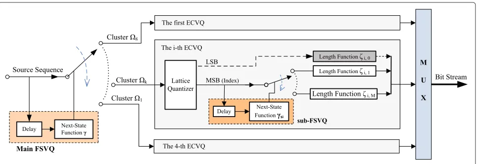
described in details in Section 4, the FS-ECVQ can be taken as a super-ECVQ, in which multiple component ECVQs are contained and all of them are combined to a FSVQ. Thus, the FS-ECVQ is composed of two steps. The first step is to split the source sequence into multi-ple clusters using the FSVQ (main FSVQ), and the second step is to apply a dedicated conventional ECVQ to each cluster. Suppose that the largest available vector dimen-sion is 8, the whole coding scheme of a FS-ECVQ can be demonstrated as Figure 1.
3.1 Main FSVQ
The major function of the main FSVQ is to partition the input space into four non-overlapped clusters according to the four states contained. For each resulting cluster, a component ECVQ is constructed holding a different vector dimension and different memory requirements. By this means, the total memory requirements could be efficiently decreased. The state transition is determined by a next-state function, which is the key component of the main FSVQ. In the following part of this section, we will mainly discuss the construction of the next-state function.
The next-state function of the main FSVQ is built on the dependencies among audio MDCT coefficients. In prac-tice, audio signals are usually divided into a series of time intervals (often referred to as ‘frames’) due to their long-term time-varying property, and over a specified frame they are assumed to be stationary. Thus, as an expres-sion of the audio signal in MDCT domain, there are high dependencies among the MDCT coefficients of the adja-cent frames as well as among the coefficients within one frame. As a result, based on the inter- and intra-frame correlations, the MDCT coefficients of current frame could be estimated through prediction methodology. In our work, the audio MDCT coefficient frames are fur-ther divided into small blocks, and then, by estimating the
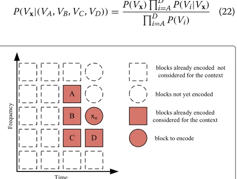
shape properties of these blocks among multiple sequen-tial frames, the next-state function is constructed in order to exploit both the intra- and inter-frame dependencies. In fact, within an audio MDCT coefficient sequence, the occurrence frequency of a block is highly related to its shape features. Suppose the block size is 4, then the rela-tionship of the shape feature and the occurrence of a block are demonstrated in Figure 2.
To characterize the shape of a block, three statistical parameters block energy,e, block deviation,σ, and block skewness,g, are employed in our work. Letμbe the mean value of blockx. Then the parameterse,σ, andgcan be written as
e= 1
N
N
i=1
x2i (18)
σ= 1 N
N
i=1
(xi−μ)2 (19)
g= 1
N
N
i=1(xi−μ)3
1
N N
i=1(xi−μ)2
3/2 (20)
wherexiandNare theith element and the length of block
x, respectively. To describe the shape feature of blockxin a simplified form, a new statistical parameter,Vx, is defined,
which is given as
Vx=(σ+e)·(1+log(1+ |g|)). (21)
Once a source sequence is split into a series of blocks, the value ofVx will be calculated for each block. Thus,
a mapping can be established between the Vx set,
com-posed of all the possible values ofVx, and the input space . Then, by splitting the possible values ofVxinto two
segments, we can partition the input space into two clusters, k and Ck. Here, k denotes the dimension of
Figure 2Three typical block shapes within an audio MDCT coefficient sequence.The blocks appeared(a)scarcely,(b)moderately, and(c) frequently.
cluster k. To implement the split, a threshold VT is
employed, whose value is obtained by maximizing the coding gain of the FS-ECVQ under the constraint of the total memory requirements using the training data. As for the two resulting clusters,k is supposed to contain the blocks occurring relatively frequently, whereasCk is assumed to hold those occurring relatively scarcely.
To construct the next-state function, four previous blocks,A, B, C, and D, which are adjacent to the cur-rent block, x, can be employed [29]. For simplicity, we assume that the current block and its previous neighbors form a Markov chain [26]. The relative positions of all these blocks are demonstrated in Figure 3. Assume that the shape parameters of the four adjacent blocks are inde-pendent measurements, then according to the research done by Nasrabadi et al. [30], the conditional joint poste-rior probability, which the next-state function is built on, can be given as
P(Vx|(VA,VB,VC,VD))=
P(Vx)Di=AP(Vi|Vx) D
i=AP(Vi)
(22)
Figure 3The input blockxand the previously encoded adjacent blocksA,B,C, andD.These blocks are used to obtain the current statesby the next-state function of the main FSVQ.
whereVxandViare the shape parameters of blockxand its four neighbors A, B, C, and D, respectively. Sup-pose that P(Vx) andP(Vi) are measured independently and considered to be equal, then probabilityP(Vi|Vx)will be equal to probabilityP(Vx|Vi), which represents a con-ditional probability of the parameterVx given one of its
neighborsVi, fori=A, B,C, and D, and can be obtained through recording all the possible cluster pairs occurring together using the training data. Assume that all the shape parameters obey the same probability distribution, then the conditional joint probability,P(Vx|(VA,VB,VC,VD)), will only depend on the four conditional probabilities
P(Vx|Vi), fori = A, B, C, andD, and the other parame-ters in (22) will be constant for any input block. Therefore, we can build the next-state function (6) on these four con-ditional probabilities, and the current state of the main FSVQ,s, can be given by
s=γ (VA,VB,VC,VD)= max
x∈{k,Ck} D
i=A
P(Vx|Vi) (23)
which denotes an estimation of the cluster to which the current block is most likely to be classified.
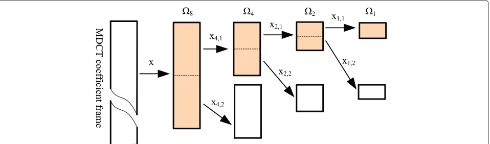
To split the source sequence into smaller clusters, a pyramidal decomposing algorithm is employed, as demonstrated in Figure 4. In this algorithm, a block,x, is first separated from the source sequence, whose length is set to be the largest available vector dimension, supposed to be 8. Then, the current statesof the obtained blockx, which is calculated through (23), is compared with a given threshold,T8. If current statesis lower thanT8, blockx
will be taken as an element belonging to cluster8. Else, it would be equally decomposed into two smaller blocks,
Figure 4Pyramidal decomposing procedure of input vector (block)x.It is split into subvectors with an optimal vector dimension.
lower thanT4, the blockx(1)4 will be taken as an element
belonging to cluster4. Else, it will be decomposed once more. This procedure continues iteratively until the lowest available vector dimension, supposed to be 1, is reached. Since each threshold can be regarded as the occurrence frequency of a block, then the current blocks considered to be with low-occurrence frequency, will be split iter-atively, until a suitable vector dimension is found. The whole procedure is summarized in Algorithm 1.
Algorithm 1The method to split the source sequence into 4 non-overlapped clusters.
Require:
The source sequence, the largest available vector dimension 8, and the thresholdsTk, fork∈ {8, 4, 2, 1};
Ensure:
1: Set the vector dimensions of current block,x, and its four previous neighbors,A,B,C, andD, to be 8; And setk=8.
2: Calculate current state,s, according to (23);
3: Ifs≥Tk, thenk←k/2; else goto step 5;
4: Equally split current block xinto x(1)k andx(2)k , and
let x(1)k be the new current block x. And then, set the dimension of its four previous neighbors,
A, B, C, andDall to bek, and go back to step 2;
5: Clusterkis selected and the current blockxbelongs tok;
6: If the source sequence is unfinished, go back to step 1; 7: return Clusterk, fork=8, 4, 2, 1;
At beginning, there is no previous block, and therefore, an original state,s0, ought to be initialized by the main
FSVQ.
3.2 ECVQ
Based on the research done by Gray et al. [25], in our work,
Zn lattice quantizer and arithmetic coder are selected as
the lattice quantizer and the length function of each com-ponent ECVQ, respectively. Unlike conventional ECVQ [15,17], where all the vector indices generated from the lattice quantizer share a same length function regardless of their possible differences, in our work multiple length functions are available and the optimal one is selected by another FSVQ (sub-FSVQ) for each generated vec-tor index. Moreover, to improve the robustness and, at the same time, decrease the memory requirements of each component ECVQ, the design of sub-FSVQ is opti-mized and an iterative method to merge the similar length functions is proposed.
The length functions are implemented by an arithmetic coder, which are based on the pdf model of the input index. Hence, the main work of the sub-FSVQ is to search for the optimal one among a predesigned collection of pdf models based on the information obtained from previous indices.
3.2.1 Lattice quantizer
The issue whether an optimal ECVQ has a finite or infinite number of codevectors has been in-depth investigated by Gyärgy and Linder [31]. They found that ECVQ has a finite number of codevectors only if the tail of the source distribution is lighter than the tail of a Gaussian distri-bution. With respect to the probability distribution of an audio MDCT coefficient sequence, Yu et al. [32] show that the generalized Gaussian function with distribution parameterr=0.5 provides a good approximation. More-over, in practice, the possible values of the audio MDCT coefficients are always finite and concentrated in a finite range. Therefore, in our work, all codevectors of the lattice quantizer are simply constrained in the range
P{||X|| ≤t0} ≥p0 (24)
where Xdenotes an input vector, andt0 andp0are two
Since all the codevectors are constructed within the range (24), the input vectors outside the range will suf-fer a larger quantization loss than those inside the range. Such circumstances are usually required to be avoided for audio MDCT coefficients quantization. To keep the pos-sible quantization error constant, the input vector which falls outside the range (24) will be split into two parts, the least significant bits (LSB) and the most significant bits (MSB), and then the two parts are encoded separately. Letx = (x1,. . .,xk)be a candidate vector, whose vector dimension isk. Assume that after each split the generated MSB and LSB are denoted byx∗andBi=(bi0,bi1,. . .,bik), respectively, whereidenotes thei-th split. To indicate an overflow happens, a symbol,escape symbol, is employed. The whole procedure is demonstrated in Algorithm 2.
Algorithm 2The split of an overflowed vectorxinto the LSB and MSB parts.
Require:
The overflowed vectorx= (x1,. . .,xk)and an array,
Bi, fori=0, 1, 2,. . ., to preserve the resulting LSBs.
Ensure:
1: SetB0=0 andi=0;
2: If ||x|| ≤ t0, then exit; {not overflowed, no split is
needed}
3: Split vectorxinto the LSB and MSB parts:
Bi=(bi0=x0& 1,. . .,bik=xk& 1),
x∗=(x01,. . .,xk 1);
And then,i←i+1 and setBi=0;
4: If ||x∗|| > t0, x ← x∗, go back to step 3; {still
overflowed, split it again}
5: MSB is the resulting vector x∗ and LSBs areBi, for
i=0,. . .,I, whereIis the number of split;
6: return The LSB sequenceB0,. . .,BI, MSBx∗, andI, which denotes the number ofescape symbol;
3.2.2 Sub-FSVQ
This FSVQ is used to search for the optimum in a pre-designed collection of length functions, which are used to encode the current vector index generated from the lat-tice quantizer. The next-state function of the sub-FSVQ,
γsi, is built on the four previous indexesIA, IB, IC, and
ID, adjacent to the current input, Ix. Since the ECVQ
holds a finite number of codevectors, the simplest way to construct the next-state function is to enumerate all the possible combinations of the four neighbors, each denot-ing a certain state. But with the increase of the number of codevectors, the possible number of current states will be extremely large, and thus, the memory requirements and the computation cost skyrocket.
To reduce the number of possible current states, the different dependencies between the current index and its
four previous neighbors must be taken into account. In practice, less emphasis is placed on indicesIAandICthan on indicesIBandID. This is due to the fact that among the four neighbors, current vectorxis less relevant to vectors
AandCthan to vectorsBandD. Thus, we apply the oper-ation|| · ||2to vectorsAandC, so as to reduce the number
of their possible values.
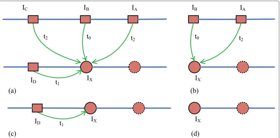
The location of the current vector should also be consid-ered. The frame, current vector located, can be generally classified into two types: the normal frame and the reset frame. In addition, within a frame the current vector can be located at the normal position or the starting position. Thus, there exist four cases, as demonstrated in Figure 5. Specially, if the current vector is located at the starting position of a reset frame, there will be no adjacent vector to build the next-state function, then a special state,ss0,
should be assigned.
As a result, the next-state function of the sub-FSVQ can be written as
ssi=γsi(IB,ID,I||A||2,I||C||2)
= ⎧ ⎪ ⎪ ⎪ ⎪ ⎨ ⎪ ⎪ ⎪ ⎪ ⎩
t0IB+t1ID+t2(I||C||2+I||A||2) Case:(a)
t0IB+t2I||A||2 Case:(b)
t1ID Case:(c)
ss0 Case:(d)
(25)
where i denotes that the sub-FSVQ belongs to the i-th ECVQ andt0,t1, andt2are three constants making each
combination of the four indices corresponding to a differ-ent currdiffer-ent state. This is feasible since for an audio MDCT coefficient sequence, the values of the four variables,IB,
ID, I||A||2, and I||C||2, are all finite, and then according
to their maximum possible values, it is easy to find the possible values of the three constants.
3.2.3 Length function
The length functions are realized by an arithmetic coder holding multiple pdf models. There are two difficulties in building an optimal arithmetic coder for an optimal ECVQ. First, the memory requirements for saving the pre-designed pdf models will become infeasible as the number of states derived from (25) increases. Second, as the vol-umes of the partitions split by the sub-FSVQ shrink, the available data may not provide credible pdf estimation. Popat and Picard [33] proposed a solution to the sec-ond problem using a Gaussian mixture model (GMM) for describing the source pdf. Thus, this work mainly focuses on reducing the memory requirements for saving the pdf models necessary for the arithmetic coder.
Figure 5Possible previous adjacent indexes used to calculate the current statessiby sub-FSVQ in four situations.(a)Normal frame and normal position.(b)Normal frame but starting position.(c)Reset frame and normal position.(d)Reset frame but starting position.
take place. Letg be the true pdf of the input signal and suppose thatgis its support. Assume that{Sm;m∈U}, whose corresponding pdf model is{gm;m ∈ U}forU = {1,. . .,M}, is a finite partition ofg and thatPg(Sm) ≤ 0 for all m. Assume also that model gm is replaced by another model,gn, then according to (17) the mismatch of the pdf model pair,gmandgn, denoted bydmis(m,n), can
be given as
dmis(m,n)=
Sm
ρmgm(x)ln
gm(x)
gn(x)
dx
=ρmI(gm||gn) (26)
whereρm, which equals to the probabilityPg(Sm), is the weight of model gm. Thus, the mismatch dmis can be
seen as a distance measure of a pdf model pair. The more similar the two models are, the smaller is the mis-match. Therefore, we can efficiently decrease the memory requirements for saving the pdf models by merging the model pairs, which hold small enough mismatches, into a new pdf model with a negligible loss of the coding performance.
For a pdf model collection, once we have obtained the
dmis values of each model pair, we can merge the ones
with minimal dmisvalues into a new pdf model so as to
reduce the memory requirements. If the memory size is still above the requirements, the mergence of the simi-lar pdf models should be continued. But once a new pdf model is generated, the mismatches among pdf models should be updated first. And then, a new merge can be
executed. The whole procedure will be carried out iter-atively, until the memory size reaches the requirements. Once the final pdf models are obtained, a remapping between these models and their corresponding states is needed.
4 Results
In USAC [34], an up-to-date MPEG standardization, MDCT plays an important role [35]. In the USAC encoder, the MDCT coefficients are firstly companded with a power low function before scalar quantization, achieving in effect a non-uniform scalar quantization. And then, the residuals are further entropy coded. To improve the per-formance of MDCT coefficients quantization and coding, a novel scheme [29], which combined a scalar quantiza-tion with a context-based entropy coding, was developed in the USAC. In this new scheme, the input tuples (blocks) were first quantized by a scalar quantizer (SQ), and then the generated tuple indices were further encoded through a context-based arithmetic encoder. In the USAC final version (FINAL), the tuple length of this scheme was selected to be 2, in order to decrease the total memory requirements.
To make an easy comparison with the FINAL, the FS-ECVQ was divided into two parts, SQ, which was formed by merging the scaling steps contained in the three com-ponent ECVQs and constructed just the same as the one in the FINAL, and the core module of FS-ECVQ, which was referred to FS-ECVQ for simplicity. Thus, the FS-ECVQ and the FINAL would share the same source sequence and the same quantization error and only differ in their coding performance. Therefore, the remainder of this section was mainly focused on evaluating the coding performance of the FINAL and the FS-ECVQ.
4.1 Memory requirements
The total memory requirements of the FINAL and the FS-ECVQ were demonstrated in Table 1. From Table 2, it could be seen that the number of codevectors in FS-ECVQ and FINAL were 85 and 17, respectively. This implied that the equivalent vector dimension of FS-ECVQ would be slightly higher than 2, the dimension of FINAL. Generally, fewer codevectors would lead to a smaller num-ber of vector indices and a smaller memory requirements of each cumulative distribution function (cdf ) model. Thus, compared with the FINAL, the FS-ECVQ held a much higher memory requirements for preserving the cdf models.
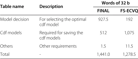
Compared with FINAL, the FS-ECVQ was less memory exhausting in cdf model decision. This was mainly due to the two FSVQs (main FSVQ and sub-FSVQ), which adap-tively reshaped the input blocks and merged the states with similar cdf models to be a new one, while at the same time no side information was needed to be transmit-ted. Thus, the number of states needed to be conserved contained in sub-FSVQ would be much fewer than those contained in the context-model of the FINAL. As a result, the FS-ECVQ further reduced the total memory require-ments of the FINAL by up to 11.3%.
The number of codevectors (codebook size) and the memory requirements for saving the cdf models of FINAL and FS-ECVQ were demonstrated in Table 2. It could be seen that the FS-ECVQ employed three different code-books, whose dimensions were 4, 2, and 1, respectively.
Table 1 Memory requirements for the two methods: FINAL and FS-ECVQ
Table name Description Words of 32 b FINAL FS-ECVQ
Model decision For selecting the optimal cdf model
927.5 192
Cdf models Required for saving the cdf models
512 1,075
Others Other requirements 1.5 11.5
Total - 1,441.0 1,278.5
Table 2 Number of codevectors, models, and memory requirements for FINAL and FS-ECVQ
Codebook FINAL FS-ECVQ
Vector Model ROM Vector Model ROM
Dimension 1 - - - 10 27 108
Dimension 2 17 64 512 26 31 264
Dimension 4 - - - 49 27 703
Total 17 64 512 85 85 1,075
Among these codebooks, the 4-dimensional codebook was assigned the largest number of codevectors, whereas the 1-dimensional one was assigned the least. Through this means, the equivalent vector dimension of the FS-ECVQ would be reduced, and therefore, its memory requirements would be efficiently decreased.
4.2 Average computational complexity
The average computational complexities of the FINAL and the FS-ECVQ, whose units were the weighted million operations per second (WMOPS), were shown in Table 3. From this table, it could be seen that the FS-ECVQ and FINAL held a similar average complexity. The average complexity of FS-ECVQ was mainly due to its main FSVQ. In FS-ECVQ, the main FSVQ was used to estimate which cluster the current block would be classified into accord-ing to the shape parameters of its four previous adjacent blocks. To obtain these shape parameters, cubic terms were introduced which obviously increased the total com-putational complexity.
As the cubic terms usually led to a large computation, to reduce the computational complexity, a look-up table was employed in the FS-ECVQ so that the FS-ECVQ held a similar computational complexity as the FINAL. In prac-tice, the size of the look-up table was dependent on the selection of the threshold of the main FSVQ. In our work, to calculate the threshold of current block, four previous neighbors were employed. Since the current block and its four neighbors were highly correlated and usually hold a similar envelope shape, the largest element of all the code-vectors could be constrained to a small value, such as 8. Thus, the size of the look-up table for storing the cubic terms would be very small, about two words.
4.3 Rate performance
Nine audio items, covering speech, music, and mixed speech/music signals, were used for the training of the
Table 3 Average complexity numbers for decoding 32 kbps stereo reference quality bitstreams for quantizers FINAL and FS-ECVQ
Operating mode USAC-FINAL FS-ECVQ
main-FSVQ, sub-FSVQ, and cdf models, of which the bitrates ranged from 12 to 64 kbps, and the length of every item was about 2 h. And among them, four were mono while the others were stereo items. Another nine audio items, also covering speech, music, and mixed speech/music signals, were chosen as the testing set for the FINAL and the FS-ECVQ, of which the bitrates ranged from 12 to 64 kbps and the length of every item was about 3 min. Among them, four were mono while the others were stereo. The testing results were shown in Table 4, where the percentage column represented the increment of the coding gain of the current method over the FINAL. The table demonstrated that the FINAL and the FS-ECVQ achieved a similar coding performance in all the nine items. This denoted that the FINAL and the FS-ECVQ both could efficiently remove the redundancies within audio MDCT coefficient sequences. Moreover, both FINAL and FS-ECVQ obtained more coding gains in the low bitrate items than in the high bitrate items. These phenomena were mainly due to the fact that the nine items have different pdf of MDCT coefficients. In FS-ECVQ, a different source distribution would lead to a different calling ratio of its three component ECVQs.
4.4 Main FSVQ
The main FSVQ split the input vectors into subvectors according to a pyramidal decomposing method, by which the MDCT coefficient sequence was partitioned into three clusters,4,2, and 1. The component ECVQs
applied on these resulting clusters were ECVQ_D4, ECVQ_D2, and ECVQ_D1, respectively. To decompose an input vector, in cluster 4 and2, the main FSVQ
would first calculate two shape parameters from the two pairs of previous adjacent blocks B, D and A, C, respectively, via their corresponding block energies and block skewness, and then, compare them with the two
Table 4 Bitrates of quantizers FINAL and FS-ECVQ for nine audio items
Operating mode FINAL FS-ECVQ
(kbps) (kbps) (%)
Test 1, 64 kbps stereo 48.59 48.77 −0.33
Test 2, 32 kbps stereo 24.56 24.55 0.04
Test 3, 24 kbps stereo 17.59 17.57 0.11
Test 4, 20 kbps stereo 14.87 14.86 0.09
Test 5, 16 kbps stereo 11.71 11.69 0.17
Test 6, 24 kbps mono 18.97 18.98 −0.05
Test 7, 20 kbps mono 15.41 15.42 −0.06
Test 8, 16 kbps mono 12.18 12.17 0.08
Test 9, 12 kbps mono 8.78 8.76 0.23
Average 19.18 19.18 0.03
thresholds, Tbd and Tac, respectively. Thus, a different combination of the thresholds would lead to a different distribution of the MDCT coefficients among the three component ECVQs, and consequently a different coding gain of the FS-ECVQ. The different combinations ofTbd andTacin the two clusters and their corresponding results were all demonstrated in Table 5. From the table, at least two points could be derived.
First, the thresholds of cluster 4 had a larger impact on the coding gain than cluster 2 did, which could be explained by the fact that the variation range of the coding gains on4was much wider than that on2. Further-more, within a level threshold Tbd had a larger impact on the coding gain than thresholdTacdid. SinceTbdand
Tac were obtained from adjacent blocksB, DandA, C, respectively, this proved the assumption thatB, Dwere more significant thanA, C.
Second, the component ECVQ, ECVQ_D4, gains than the two others. From Table 5, it could be observed that most of the MDCT coefficients were encoded by ECVQ_D4. Therefore, to obtain the optimal performance, the promotion of performance of ECVQ_D4 should be of the highest priority.
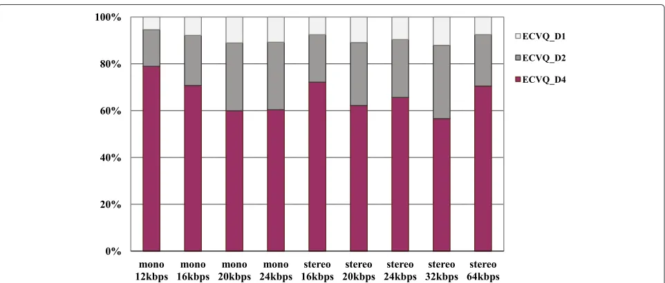
The calling ratios of the three component ECVQs in the nine testing items were demonstrated in Figure 6. It could also be observed that among all the nine items, the calling frequency of ECVQ_D4 was the highest, whereas the frequency of ECVQ_D1 was the lowest. As the vec-tor dimensions ECVQ_D4, ECVQ_D2, and ECVQ_D1, were 4, 2, and 1, respectively, the calling rations of them implied that most of the MDCT coefficients in each test-ing item were encoded by the 4-dimensional ECVQ and only a very small amount of them were encoded by the 1-dimensional one. Through this way, FS-ECVQ achieved a relatively high coding performance. Furthermore, among all the nine items, the more frequently ECVQ_D4 was called, the larger coding gains the FS-ECVQ obtained. This explained why FS-ECVQ was more efficient in cod-ing low bitrate items than the high bitrate ones.
4.5 ECVQ
As each component ECVQ contained two stages, lattice quantization and entropy coding, we would first assess the quantization stage and then, the entropy coding stage.
4.5.1 Quantization stage
Table 5 The effects on the three component ECVQs and coding gains
Pyramidal Threshold ECVQ_D4 ECVQ_D2 ECVQ_D1 Gains (%)
decomposition Tbd Tac Ratio (%) LSB (%) Ratio (%) LSB (%) Ratio (%) LSB (%)
4a 9
30
77.395 1.403 16.769 1.873 5.837 9.883 3.0626
10 79.276 1.623 14.895 2.075 5.830 9.895 2.9917
12 82.300 2.104 11.884 2.501 5.816 9.914 2.7091
17 82.517 2.159 11.669 2.529 5.814 9.916 2.6779
24 83.410 2.403 10.785 2.673 5.805 9.925 2.5094
∞ 87.733 4.947 7.728 2.672 4.539 10.129 0.9096
10
24 78.733 1.579 15.436 2.014 5.832 9.892 3.0123
27 78.836 1.588 15.333 2.025 5.831 9.893 3.0094
33 79.520 1.645 14.651 2.105 5.829 9.896 2.9834
36 79.606 1.654 14.566 2.117 5.829 9.896 2.9812
∞ 81.651 1.917 12.624 2.363 5.725 10.062 2.7537
2b 32
243 79.276 1.623
13.849 1.647 6.875 8.455 2.9771
45 14.542 1.880 6.183 9.363 3.0022
67 15.219 2.241 5.505 10.443 2.9449
75 15.496 2.436 5.228 10.950 2.8997
∞ 17.364 6.231 3.360 12.663 1.4433
65
189
79.276 1.623
14.727 2.021 5.997 9.634 2.9563
216 14.776 2.036 5.948 9.707 2.9535
249 14.922 2.085 5.802 9.941 2.9929
257 14.942 2.098 5.782 9.972 2.9916
∞ 15.537 2.548 5.817 10.975 2.8963
aSet the thresholds of
2to beTbd=65,Tac=243;bset the thresholds of4to beTbd=10,Tac=30. Meanwhile, the main FSVQ is of different thresholds in 24 kbps stereo.
higher coding gain achieved by the component ECVQ. Second, by adjusting the thresholdTbdandTac, we could achieve different occurrence frequency of LSB and thus make different trade-off between the coding gain and the memory requirements. At last, the ratio among the three LSB occurrence frequencies is correlated with the distri-bution of quantization errors among the three component ECVQs. A higher LSB occurrence frequency denoted more quantization errors distributed to the corresponding component ECVQ.
The LSB occurrence in each component ECVQ signif-icantly influenced the final coding gain of the FS-ECVQ, which could be seen from the Table 5. For an input vector, if the LSB appeared, the ECVQ would consume much more bits than that for encoding it directly. There
were two methods for reducing the appearance of LSB: to enlarge the range of the corresponding codebook or to shrink the range constrained by the threshold. However, the first method would lead to an increase in the memory requirements, while the second would degrade the cod-ing gain. Therefore, a trade-off must be made between the memory requirements and the coding gain. Among the three ECVQs, ECVQ_D4 had the least percentage of LSBs while ECVQ_D1 had the largest. By this means, the FS-ECVQ could save the memory requirements while keeping the coding gain as high as possible.
4.5.2 The length functions
In each component ECVQ, the length function was realized by an arithmetic coder, which employed the
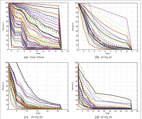
sub-FSVQ to search for the optimum in a predesigned cdf model collection. The cdf models of FINAL and FS-ECVQ were demonstrated in Figure 7. From the figure, it could be seen that the cdf model numbers of the FINAL and FS-ECVQ were 64 and 85, respectively. Essen-tially, the cdf models contained were used to fit the pdf of the MDCT coefficient sequence. A larger number of cdf models generally would provide a higher accu-racy fitting of the source pdf. Therefore, the FS-ECVQ could obtain a higher performance than the FINAL, theoretically.
Although the FINAL contained less cdf models than the FS-ECVQ did, it obtained similar coding perfor-mance to the FS-ECVQ. This was mainly owing to the cdf model selection method used in FINAL, which accu-rately selected the optimal cdf model for each input vector index. However, it was more complicated than that used in FS-ECVQ. This could be seen from the fact that the mem-ory requirements for the cdf model selection in FINAL was much larger than those in FS-ECVQ, as demonstrated in Table 1.
5 Conclusions
In this paper, an ECVQ with finite memory, called FS-ECVQ, is proposed. In the FS-FS-ECVQ, a FSVQ, namely the main FSVQ, is used to partition the source sequence into multiple non-overlapped clusters. Then to each clus-ter, an ECVQ is applied. Within each ECVQ, its length function is taken by an arithmetic coder holding mul-tiple predesigned cdf models. To select the optimal cdf model for each input vector, another FSVQ, namely the sub-FSVQ, is employed.
Owing to the main FSVQ which effectively exploits the inter-frame dependencies, the source sequence is split into multiple clusters and no side information is needed to be transmitted. Moreover, the main FSVQ assigned differ-ent vector dimensions to the resulting clusters. The more frequently a cluster appears, the higher vector dimen-sion is allocated. This helps the FS-ECVQ to efficiently reduce its total memory requirements while, at the same time, maintaining a relatively high coding performance. Finally, for each input vector, the sub-FSVQ selects the best matching cdf model, which adds robustness to the FS-ECVQ.
There are multiple ways to realize the proposed FS-ECVQ. First of all, if the quantizing errors generated from the lattice quantizer are directly discarded, then the FS-ECVQ is equivalent to an ordinary FS-ECVQ. However, if the quantizing errors are taken as the LSBs and encoded by an additional length function, the FS-ECVQ will be equal to an uniform quantizer. In addition, if the quantization steps of all the component ECVQs are separated from the FS-ECVQ, then the FS-ECVQ becomes an entropy encoder. The FS-ECVQ can also be used in coding the
speech, image, and video signals, and even any other source sequence with non-uniform distribution.
Competing interests
The authors declare that they have no competing interests.
Acknowledgements
The authors wish to thank the anonymous reviewers for their detailed comments and suggestions, which have been extremely helpful in improving the clarity and quality of this paper. This work was supported by the National Natural Science Foundation of China under Grant No. 61171171.
Received: 18 December 2013 Accepted: 16 April 2014 Published: 12 May 2014
References
1. A Gersho, RM Gray,Vector Quantization and Signal Compression. (Wiley, New York, 1994)
2. S So, KK Paliwal, Efficient product code vector quantisation using the switched split vector quantiser. Digit Signal Process.17, 138–171 (2007) 3. R Gray, D Neuhoff, Quantization. Inform. Theory, IEEE Trans.44(6),
2325–2383 (1998)
4. A Subramaniam, B Rao, PDF optimized parametric vector quantization of speech line spectral frequencies. Speech Audio Process IEEE Trans.11(2), 130–142 (2003)
5. S So, K Paliwal, Multi-frame GMM-based block quantisation of line spectral frequencies for wideband speech coding, inProceedings in IEEE International Conference on Acoustics, Speech, and Signal Processing, (ICASSP ’05), vol. 1(Philadelphia, March 2005), pp. 121–124
6. K Paliwal, B Atal, Efficient vector quantization of LPC parameters at 24 bits/frame. Speech Audio Process IEEE Trans.1, 3–14 (1993)
7. M Bouzid, S Cheraitia, M Hireche, Switched split vector quantizer applied for encoding the LPC parameters of the 2.4 Kbits/s MELP speech coder, in
7th International Multi-Conference on Systems Signals and Devices(Amman, Jordan, June 2010), pp. 1–5
8. J Leis, S Sridharan, Adaptive vector quantization for speech spectrum coding. Digit Signal Process.9(2), 89–106 (1999)
9. S Chatterjee, T Sreenivas. Optimum switched split vector quantization of LSF parameters.Signal Process.88(6), 1528–1538 (2008)
10. F Nordin, T Eriksson, On split quantization of LSF parameters, in
Proceedings on IEEE International Conference on Acoustics, Speech, and Signal Processing (ICASSP ’04), vol. 1(Montreal, May 2004), pp. I–157–60 11. S So, KK Paliwal, A comparative study of LPC parameter representations
and quantisation schemes for wideband speech coding. Digit Signal Process.17, 114–137 (2007)
12. S Chatterjee, T Sreenivas, Gaussian mixture model based switched split vector quantization of LSF parameters, inIEEE International Symposium on Signal Processing and Information Technology(Giza, December 2007), pp. 1054–1059
13. Y Lee, W Jung, MY Kim, GMM-based KLT-domain switched-split vector quantization for LSF coding. Signal Process Lett. IEEE.18(7), 415–418 (2011)
14. S Chatterjee, T Sreenivas, Switched conditional PDF-based split VQ using gaussian mixture model. Signal Process Lett. IEEE.15, 91–94 (2008) 15. P Chou, T Lookabaugh, R Gray, Entropy-constrained vector quantization.
Acoustics Speech Signal Process. IEEE Trans.37, 31 –42 (1989)
16. T Lookabaugh, R Gray, High-resolution quantization theory and the vector quantizer advantage. Inform Theory IEEE Trans.35(5), 1020–1033 (1989) 17. D Zhao, J Samuelsson, M Nilsson, On entropy-constrained vector
quantization using gaussian mixture models. Commun IEEE Trans.56(12), 2094–2104 (2008)
18. A Vasilache, Rate-distortion models for entropy constrained lattice quantization, inIEEE International Conference on Acoustics Speech and Signal Processing, (ICASSP ’10)(Dallas, March 2010), pp. 4698–4701 19. J Foster, R Gray, M Dunham, Finite-state vector quantization for waveform
coding. Inform Theory IEEE Trans.31(3), 348–359 (1985) 20. BS Andras Cziho, IL ETC, An optimization of finite-state vector
quantization for image compression. Signal Process Image Commun.
15(6), 545–558 (2000)
22. RF Chang, YL Huang, Finite-state vector quantization by exploiting interband and intraband correlations for subband image coding. Image Process IEEE Trans.5(2), 374–378 (1996)
23. S Jiang, R Yin, P Liu, A finite-state entropy-constrained vector quantizer for audio MDCT coefficients coding, inInternational Conference on Audio, Language and Image Processing, (ICALIP 2012)(Shanghai, July 2012), pp. 218–223
24. ISO/IEC JTC1/SC29/WG11, Call for proposals on unified speech and audio coding (2007). [http://mpeg.chiariglione.org/standards/mpeg-d/unified-speech-and-audio-coding]
25. R Gray, T Linder, J Li, A Lagrangian formulation of Zador’s
entropy-constrained quantization theorem. Inform Theory IEEE Trans.
48(3), 695–707 (2002)
26. N Nasrabadi, S Rizvi, Next-state functions for finite-state vector quantization. Image Process IEEE Trans.4(12), 1592–1601 (1995) 27. R Gray, J Li, On Zador’s entropy-constrained quantization theorem, in
Proceedings on Data Compression Conference, (DCC 2001)(Snowbird, March 2001), pp. 3–12
28. R Gray, T Linder, Mismatch in high-rate entropy-constrained vector quantization.Inform. Theory IEEE Trans.49(5), 1204–1217 (2003) 29. G Fuchs, V Subbaraman, M Multrus, Efficient context adaptive entropy
coding for real-time applications, inIEEE International Conference on Acoustics, Speech and Signal Processing, (ICASSP ’11)(Prague, May 2011), pp. 493–496
30. N Nasrabadi, C Choo, Y Feng, Dynamic finite-state vector quantization of digital images. Commun IEEE Trans.42(5), 2145–2154 (1994)
31. A Gyorgy, T Linder, P Chou, B Betts, Do optimal entropy-constrained quantizers have a finite or infinite number of codewords Inform Theory IEEE Trans.49(11), 3031–3037 (2003)
32. R Yu, X Lin, S Rahardja, C Ko, A statistics study of the MDCT coefficient distribution for audio, inIEEE International Conference on Multimedia and Expo, (ICME ’04) vol. 2(Taipei, June 2004), pp. 1483–1486
33. K Popat, R Picard, Cluster-based probability model and its application to image and texture processing. Image Process IEEE Trans.6(2), 268–284 (1997)
34. ISO/IEC JTC 1/SC 29N11510, Information technology - MPEG audio technologies Part 3: unified speech and audio coding (2010). [http:// mpeg.chiariglione.org/standards/mpeg-d/unified-speech-and-audio-coding]
35. M Neuendorf, P Gournay, M Multrus, J Lecomte, B Bessette, R Geiger, S Bayer, G Fuchs, J Hilpert, N Rettelbach, R Salami, G Schuller, R Lefebvre, B Grill, Unified speech and audio coding scheme for high quality at low bitrates, inIEEE International Conference on Acoustics, Speech and Signal Processing, (ICASSP ’09)(Taipei, April 2009), pp. 1–4
doi:10.1186/1687-4722-2014-22
Cite this article as:Jianget al.:A memory efficient finite-state source coding algorithm for audio MDCT coefficients.EURASIP Journal on Audio, Speech, and Music Processing20142014:22.
Submit your manuscript to a
journal and benefi t from:
7Convenient online submission 7Rigorous peer review
7Immediate publication on acceptance 7Open access: articles freely available online 7High visibility within the fi eld
7Retaining the copyright to your article