R E S E A R C H
Open Access
N
-dimensional
N
-microphone sound source
localization
Ali Pourmohammad
*and Seyed Mohammad Ahadi
Abstract
This paper investigates real-timeN-dimensional wideband sound source localization in outdoor (far-field) and low-degree reverberation cases, using a simpleN-microphone arrangement. Outdoor sound source localization in different climates needs highly sensitive and high-performance microphones, which are very expensive. Reduction of the microphone count is our goal. Time delay estimation (TDE)-based methods are common forN-dimensional wideband sound source localization in outdoor cases using at leastN+ 1 microphones. These methods need numerical analysis to solve closed-form non-linear equations leading to large computational overheads and a good initial guess to avoid local minima. Combined TDE and intensity level difference or interaural level difference (ILD) methods can reduce microphone counts to two for indoor two-dimensional cases. However, ILD-based methods need only one dominant source for accurate localization. Also, using a linear array, two mirror points are produced simultaneously (half-plane localization). We apply this method to outdoor cases and propose a novel approach forN-dimensional entire-space outdoor far-field and low reverberation localization of a dominant wideband sound source using TDE, ILD, and head-related transfer function (HRTF) simultaneously and onlyNmicrophones. Our proposed TDE-ILD-HRTF method tries to solve the mentioned problems using source counting, noise reduction using spectral subtraction, and HRTF. A special reflector is designed to avoid mirror points and source counting used to make sure that only one dominant source is active in the localization area. The simple microphone arrangement used leads to linearization of the non-linear closed-form equations as well as no need for initial guess. Experimental results indicate that our implemented method features less than 0.2 degree error for angle of arrival and less than 10% error for three-dimensional location finding as well as less than 150-ms processing time for localization of a typical wideband sound source such as a flying object (helicopter).
Keywords:Sound source localization; ITD; TDE; TDOA; PHAT; ILD; HRTF
1. Introduction
Source localization has been one of the fundamental problems in sonar [1], radar [2], teleconferencing or videoconferencing [3], mobile phone location [4], naviga-tion and global posinaviga-tioning systems (GPS) [5], localizanaviga-tion of earthquake epicenters and underground explosions [6], microphone arrays [7], robots [8], microseismic events in mines [9], sensor networks [10,11], tactile interaction in novel tangible human-computer interfaces [12], speaker tracking [13], surveillance [14], and sound source tracking [15]. Our goal is real-time sound source localization in outdoor environments, which necessitates a few points to be considered. For localizing such sound sources, a far-field assumption is usual. Furthermore, our experiments
confirm that placing localization system in suitable higher heights often reduces the reverberation degree, especially for flying objects. Also, many such sound source signals are wideband signals. Moreover, outdoor high-accuracy sound source localization in different climates needs highly sensitive and high-performance microphones which are very expensive. Therefore, reduction of the number of mi-crophones is very important, which in turn leads to re-duced localization accuracies using conventional methods. Here, we intend to introduce a real-time accurate wide-band sound source localization system in low degree rever-beration far-field outdoor cases using fewer microphones.
The structure of this paper is as follows. After a litera-ture review, we explain HRTF-, ILD-, and TDE-based methods and discuss TDE-based phase transform (PHAT). In Section 4, we explain sound source angle of arrival and location calculations using ILD and PHAT. Section 5 * Correspondence:[email protected]
Electrical Engineering Department, Amirkabir University of Technology, 424 Hafez Ave., Tehran 15914, Iran
covers the introduction of TDE-ILD-based method to two-dimensional (2D) half-plane sound source localization using only two microphones. Section 6 includes simula-tion of this method for 2D cases, where according to simulation results and due to the use of ILD, we introduce source counting. In Section 7, we propose, and in Section 8, we implement our TDE-ILD-HRTF-based method for 2D whole-plane and three-dimensional (3D) entire-space sound source localization. Section 9 includes the imple-mentations. Finally conclusions will be made in Section 10.
2. Literature review
Passive sound source localization methods, in general, can be divided into direction of arrival (DOA) [16], time difference of arrival (TDOA) or TDE or interaural time difference (ITD)- [17-20], ILD- [21-24], and HRTF-based methods [25-30]. DOA-HRTF-based beamforming and sub-space methods typically need a large number of mi-crophones for estimation of narrowband source loca-tions in far-field cases and wideband source localoca-tions in near-field cases. Also, they have higher processing needs in comparison to other methods. Many localization methods for near-field cases have been proposed in the literature, such as maximum likelihood (ML), covariance approximation, multiple signal estimation (MUSIC), and estimation of signal parameters via rotational invariance techniques (ESPRIT) [16]. However, these methods are not applicable to the localization of wideband signal sources in far-field cases with small number of micro-phones. On the other hand, ILD-based methods are mostly applicable to the case of a single dominant sound source (high signal-to-noise ratio (SNR)) [21-24]. TDE-based methods with high sampling rates are commonly used for 2D and 3D high-accuracy wideband near-field and far-field sound source localization. In the case of ILD or TDE-based methods, minimum number of mi-crophones required is three for 2D positioning and four for the 3D case [17-20,31-39]. Finally, HRTF-based methods are applicable only to the case of calculating ar-rival angle in azimuth or elevation [30].
TDE- and ILD-based outdoor far-field accurate wide-band sound source localization in different climates needs highly sensitive and high-performance micro-phones which are very expensive. In the last decade, some papers were published which introduce 2D sound source localization methods using just two microphones in indoor cases using TDE- and ILD-based methods simultaneously. However, it is noticeable that using ILD-based methods requires only one dominant source to be active, and it is known that, by using a linear array in the proposed TDE-ILD-based method, two mirror points will be produced simultaneously (half-plane localization) [40]. In this paper, we apply this method in outdoor (low-degree reverberation) cases for a dominant sound source.
We also propose a novel method to have 2D whole-plane (without producing two mirror points) and 3D entire-space dominant sound source localization using TDE-, ILD-, and HRTF-based methods simultaneously (TDE-ILD-HRTF method). Based on the proposed method, a special reflector for the implemented simple microphone arrangement is designed, and source counting method is used to find that only one dominant sound source is active in the localization area.
In TDE and ILD localization approaches, calculations are carried out in two stages: estimation of time delay or intensity level differences and location calculation. Cor-relation is most widely used for time delay estimation [17-20,31-39]. The most important issue in this ap-proach is high-accuracy time delay estimation between microphone pairs. Meanwhile, the most important issue in ILD-based approach is high accuracy level difference measurement between microphone pairs [21-24]. Also, numerous results were published in the last decades for the second stage, i.e., location calculation. Equation complexities and large processing times are the import-ant obstacles faced at this stage. In this paper, we propose a simple microphone arrangement that solves both these problems simultaneously.
In the above-mentioned first stage, the classic methods of source localization from time delay estimates by de-tecting radio waves were Loran and Decca [31]. How-ever, generalized cross-correlation (GCC) using a ML estimator, proposed by Knapp and Carter [32], is the most widely used method for TDE. Later, a number of techniques were proposed to improve GCC in the pres-ence of noise [3,33-36]. As GCC is based on an ideal signal propagation model, it is believed to have a funda-mental weakness of inability to cope well with reverberant environments. Some improvements were obtained by cepstral prefiltering by Stephenne and Champagne [37]. Even though more sophisticated techniques exist, they tend to be computationally expensive and are thus not well suited for real-time applications. Later, PHAT was proposed by Omologo and Svaizer [38]. More recently, a new PHAT-based method was proposed for high-accuracy robust speaker localization, known as steered response pattern-phase or power-phase transform (SRP-PHAT) [39]. Its disadvantage is higher processing time in com-parison to PHAT, as it requires a search of a large number of candidate locations. According to the fact that in the application of this research, the number of candidate locations is much higher due to direction and distance es-timation; this disadvantage does not allow us to use it in real-time applications.
received signal level at different sensors for source localization. Due to the spatial separation of the sensors, the source signal will arrive at the sensors with different levels so that the level differences can be utilized for source localization. Sheng and Hu [41] followed by Blatt and Hero [42] have proposed different algorithms for lo-cating sources using a sensor network based on energy measurements. Birchfield and Gangishetty [22] applied ILD to sound source localization. While these works used only ILD-based methods to locate a source, Cui et al. [40] tried 2D sound source localization by a pair of microphones using TDE- and ILD-based methods simul-taneously. When the source signal is captured at the sensors, both time delay and signal level information are used for source localization. This technique is applicable for 2D localization with two sensors only. Also, due to the use of a linear array, it generates two mirror points simultaneously (half-plane localization). Ho and Sun [24] addressed a more common scenario of 3D localiza-tion using more than four sensors to improve the source location accuracy.
Human hearing system allows finding sound sources direction of arrival in 3D with just two ears. Pinnas, shoulders, and head diffract the incoming sound waves [43]. These propagation effects collectively are termed the HRTF. Batteau reported that the external ears play an important role in estimating the elevation angle of ar-rival [44]. Roffler and Butler [45], Oldfield and Parker [46], and Hofman et al. [47] have tried to find experi-mental evidence for this claim by using a Plexiglas head-band to flatten the pinna against the head [45]. Based on HRTF measuring, Brown and Duda have made an exten-sive experimental study and provided empirical formulas for the multipath delays produced by pinna [48]. Al-though more sophisticated HRTF models have been pro-posed [49], the Brown-Duda model has the advantage that it provides an analytical relationship between the multipath delays and the azimuth and elevation angles. Recently, Sen and Nehorai considered the Brown-Duda HRTF model as an example to model the frequency-dependent head-shadow effects and the multipath delays close to the sensors for analyzing a 3D direction finding system with only two sensors inspired by the human auditory system [43]. However, they did not consider white noise gain error or spatial aliasing error in their model. They computed the asymptotic frequency do-main Cramer-Rao bound (CRB) on the error of the 3D direction estimate for zero-mean wide-sense stationary Gaussian source signals. It should be noted that HRTF-based works are just able to estimate the azimuth and elevation angles [50]. In the last decades, some papers were published which tried to apply HRTF along with TDE for azimuth and elevation angle of arrival estima-tion [30]. According to this ability, we apply HRTF in
our TDE-ILD-based localization system for solving the ambiguity in the generation of two mirror location points. We named it TDE-ILD-HRTF method.
Given a set of TDEs and ILDs from a small set of mi-crophones using PHAT- and ILD-based methods, re-spectively, the second stage of a two-stage algorithm determines the best point for the source location. The measurement equations are non-linear. The most straight-forward way is to perform an exhaustive search in the so-lution space. However, this is computationally expensive and inefficient. If the sensor array is known to be linear, the position measurement equations are simplified. Carter focused on a simple beamforming technique [1]. However, it requires a search in the range and bearing space. Also, beamforming methods need many more microphones for high-accuracy source localization. The linearization solu-tion based on Taylor-series expansion by Foy [51] involves iterative processing, typically incurs high computational complexity, and for convergence, requires a tolerable ini-tial estimate of the position. Hahn proposed an approach [20] that assumes a distant source. Abel and Smith pro-posed an explicit solution that can achieve the Cramer-Rao Lower Bound (CRLB) in the small error region [52]. The situation is more complex when sensors are distrib-uted arbitrarily. In this case, emitter position is deter-mined from the intersection of a set of hyperbolic curves defined by the TDOA estimates using non-Euclidean geometry [53,54]. Finding the solution is not easy as the equations are non-linear. Schmidt has proposed a formu-lation [18] in which the source location is found as the focus of a conic passing through three sensors. This method can be extended to an optimal closed-form localization technique [55]. Delosme [56] proposed a gra-dient method for search in a localization procedure lead-ing to computation of optimal source locations from noisy TDOA's. Fang [57] gave an exact solution when the num-ber of TDOA measurements is equal to the numnum-ber of unknowns (coordinates of transmitter). This solution, however, cannot make use of extra measurements, avail-able when there are extra sensors, to improve position accuracy. The more general situation with extra measure-ments was considered by Friedlander [58], Schau and Robinson [59], and Smith and Abel [55]. These methods are not optimum in the least-squares sense and perform worse in comparison to the Taylor-series method.
solution. An initial guess close to the true solution is needed to avoid local minima. Selection of such a starting point is not simple in practice. Moreover, convergence of the iterative process is not assured. It also suffers from convergence problem and large LS computational burden as the method is iterative. Within the last few years, some papers were published on improving LS and closed-form methods [16,23,61-65]. Based on closed-form hyperbolic-intersection method, we will explain our proposed method, which using a simple arrangement of two micro-phones for 2D cases and three micromicro-phones for 3D cases, can simplify non-linear equations of this method to have a linear equation. Although there have been attempts to linearize closed-form non-linear equations through alge-braic means, such as [7,16,56,63], our proposed method with simple pure geometrical linearization needs less mi-crophones and features accurate localization and less pro-cessing time.
3. Basic methods 3.1. HRTF
Human beings are able to locate sound sources in three dimensions in range and direction, using only two ears. The location of a source is estimated by comparing dif-ference cues received at both ears, among which are time differences of arrival and intensity differences. The sound source specifications are modified before entering the ear canal. The head-related impulse response (HRIR) is the name given to the impulse response relating the source location and the ear location. Therefore, convolu-tion of an arbitrary sound source with the HRIR leads to what would have been received at the ear canal. The HRTF is the Fourier transform of HRIR and thus repsents the filtering properties due to diffractions and re-flections at the head, pinna, and torso. Hence, HRTF can be computed through comparing the original and modi-fied signals [25-29,43-50]. Consider Xc(k) being the Fourier transform of sound source signal at one ear (modified signal at either left or right ear) and Yc(k) to be that of the original signal. HRTF of that source can be found as [30]:
Hcð Þ ¼k Ycð Þk
Xcð Þk ð
1Þ
In detail:
Hcð Þk
j j ¼jYcð Þk j Xcð Þk
j j ð2Þ
argHcð Þ ¼k argYcð Þk −argXcð Þk ð3Þ
Hcð Þ ¼k jHcð Þk jejargHcð Þk: ð4Þ
In fact,Hc(k) contains all the direction-dependent and direction-independent components. Therefore, in order to have pure HRTF, the direction-independent elements have to be removed from Hc(k). If Cc(k) is the known CTF (common transfer function), then DTF (directional transfer function),Dc(k), can be found as:
Dcð Þ ¼k Yc kð Þ
Ccð ÞXk cð Þk : ð
5Þ
3.2. ILD-based localization
We consider two microphones for localizing a sound source. Signal s(t) propagates through a generic free space with noise and no (or low degree of ) reverber-ation. According to the so-called inverse-square law, the signal received by the two microphones can be modeled as [21-24,40-42]:
s1ð Þ ¼t s tð−T1Þ
d1 þn1ð Þt ð
6Þ
and
s2ð Þ ¼t s tð−T2Þ
d2 þn2ð Þt ; ð
7Þ
where d1 and d2 are the distances and T1 and T2 are time delays from source to the first and second micro-phones, respectively. Also n1(t) and n2(t) are additive white Gaussian noises. The relative time shift between the signals is important for TDE but can be ignored in ILD. Therefore, if we find the delay between the two sig-nals and shift the delayed signal in respect to the other one, the signal received by the two microphones can be modeled as:
s1ð Þ ¼t s tð Þ
d1 þn1ð Þt ð
8Þ
and
s2ð Þ ¼t s tð Þ
d2 þn2ð Þt : ð
9Þ
Now, we assume that the sound source is audible and in a fixed location. Also, it is available during the time interval [0, W] where W is the window size. The energy received by the two microphones can be ob-tained by integrating the square of the signal over this time interval [21-24,40-42]:
E1¼∫wos21ð Þdtt ¼
1
d21
∫w
os2ð Þt dtþ∫own21ð Þdtt ð10Þ
E1¼∫wos22ð Þdtt ¼
1
d22
∫w
According to (10) and (11), the received energy de-creases in relation to the inverse of the square of the dis-tance to the source. These equations lead us to a simple relationship between the energies and distances:
E1⋅d21 ¼E2⋅d22þη; ð12Þ
where η¼∫wo d21n21ð Þ þt d 2 2n22ð Þt
dt is the error term. If (x1,y1) is the coordinates of the first microphone, (x2,y2) is the coordinates of the second microphone and (xs,ys) is the coordinates of the sound source with respect to the origin located at array center, then:
d1¼
ffiffiffiffiffiffiffiffiffiffiffiffiffiffiffiffiffiffiffiffiffiffiffiffiffiffiffiffiffiffiffiffiffiffiffiffiffiffiffi
x1−xs ð Þ2þ
y1−ys ð Þ2
q
ð13Þ
d2¼
ffiffiffiffiffiffiffiffiffiffiffiffiffiffiffiffiffiffiffiffiffiffiffiffiffiffiffiffiffiffiffiffiffiffiffiffiffiffiffi
x2−xs ð Þ2þ
y2−ys ð Þ2
q
: ð14Þ
Now using (12), (13), and (14), we can localize the sound source (Section 4.1.).
3.3. TDE-based localization
Correlation-based methods are the most widely used time delay estimation approaches. These methods use the following simple reasoning for the estimation of time delay. The autocorrelation function of s1(t) can be writ-ten in time domain as [17-20,31-39]:
Rs1s1ð Þ ¼τ ∫
þ∞
−∞s1ð Þt ⋅s1ðt−τÞdt: ð15Þ
Dualities between time and frequency domains for autocorrelation function of s1(t) with the Fourier trans-formS1(f), results in frequency domain presentation as:
Rs1s1ð Þ ¼τ ∫þ−∞∞S1ð Þf ⋅S2ð Þef j
2πfτdf: ð16Þ
According to (15) and (16), if the time delayτis zero, this function's value will be maximized and will be equal to the energy of s1(t). The cross-correlation of two sig-nalss1(t) ands2(t) is defined as:
Rs1s2ð Þ ¼τ ∫þ−∞∞S1ð Þf ⋅S2ð Þef j2πfτdf: ð17Þ
If s2(t) is considered to be the delayed version of s1(t), this function features a peak at the point equal to the time delay. This delay can be expressed as:
τ12¼argmaxτRs1s2ð Þτ : ð18Þ
In an overall view, the time delay estimation methods are as follows [17-20,31-39]:
Correlation-Based Methods: Cross-Correlation (CC), ML, PHAT, Average Square Difference Function (ASDF)
Adaptive Filter-Based Methods: Sync Filter, LMS.
Advantages of PHAT are accurate delay estimation in the case of wideband and quasi-periodic/periodic signals, good performance in noisy and reflective environments, sharper spectrum due to the use of better weighting function and higher recognition rate. Therefore, PHAT is used in cases where signals are detected using arrays of microphones and additive environmental and reflect-ive noises are observed. In such cases, the signal delays cannot be accurately found using typical correlation-based methods as the correlation peaks cannot be pre-cisely extracted. PHAT is a cross-correlation-based method used for finding the time delay between the sig-nals. In PHAT, similar to ML, weighting functions are used along with the correlation function, i.e.,
ϕPHATð Þ ¼f
1
Gs1s2ð Þf
j j; ð19Þ
where Gs1s2ð Þf is the cross-correlation-based power spectrum. The overall function used in PHAT for the es-timation of delay between two signals is defined as:
Rs1s2ð Þ ¼τ ∫
þ∞
−∞ϕPHATð Þf ⋅Gs1s2ð Þef j2πfτdf ð20Þ DPHATð Þ ¼f argmaxτRs1s2ð Þτ ; ð21Þ
whereDPHATis the delay calculated using PHAT.Gs1s2ð Þf is found as:
Gs1s2ð Þ ¼f ∫þ−∞∞rs1s2ð Þeτ j2πfτdf ð22Þ
where
rs1s2ð Þ ¼τ E s½1ð Þst 2ðtþτÞ: ð23Þ
4. ILD- and PHAT-based angle of arrival and location calculation methods
4.1. Using ILD method
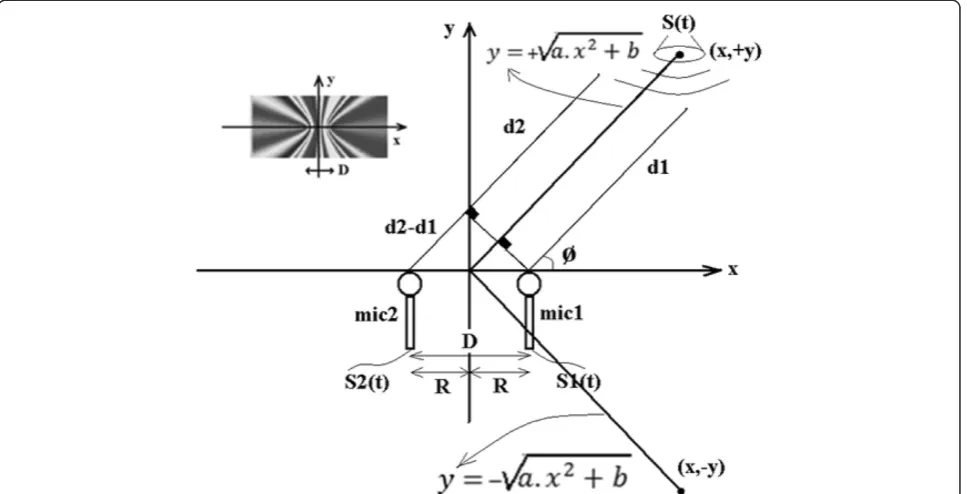
Assuming two microphones are on x-axis and have a distance ofR(R=D/2) from origin (Figure 1), we can re-write (13) and (14) as:
d1¼
ffiffiffiffiffiffiffiffiffiffiffiffiffiffiffiffiffiffiffiffiffiffiffiffiffiffiffi
R−xs ð Þ2þ
ys2
q
ð24Þ
d2¼
ffiffiffiffiffiffiffiffiffiffiffiffiffiffiffiffiffiffiffiffiffiffiffiffiffiffiffiffiffiffi −R−xs
ð Þ2þ
ys2
q
: ð25Þ
Therefore, we can rewrite (12) as:
E1 E2 ⋅d
2 1¼d
2
2þðη=E2Þ: ð26Þ
Assumingm¼E1E2andn=η/E2, (26) is written as:
Usingxandyinstead ofxsandys, (27) will become:
x2− 2R mð þ1Þ m−1
xþy2¼ n m−1−R
2 ð28Þ
x−R mð þ1Þ m−1
2
þy2¼ 1 m−1 nþ
4m m−1R
2
ð29Þ
x−k ð Þ2þ
y2¼l
k¼R mð þ1Þ m−1 l¼ 1
m−1 nþ
4m
m−1R 2
:
8 > > > > < > > > > :
ð30Þ
Therefore, source location is on a circle with center coordinates (k, 0) and radius pffiffil . Now, using a new microphone to find a new equation, in combination with one of the first or second microphones, helps us to have another circle which leads to source location with differ-ent cdiffer-enter coordinates and differdiffer-ent radii relative to the first circle. Intersection of the first and second circles gives us source locationxandy[22,40].
4.2. Using PHAT method
Assuming a single frequency sound source with a wave-length equal to λ to have a distance from the center of two microphones equal to r, this source will be in far-field if [51-65]:
r>2D 2
λ ; ð31Þ
where D is the distance between two microphones. In the far-field case, the sound can be considered as having the same angle of arrival to all microphones, as shown in Figure 1. Ifs1(t) is the output signal of the first micro-phone and s1(t) is that of the second microphone (Figure 1), taking into account the environmental noise, and according to the so-called inverse-square law, the signal received by the two microphones can be modeled as (6) and (7). The relative time shift between the signals is important for TDOA but can be ignored in ILD. Also, the attenuation coefficients (1/d1and 1/d2) are important for ILD but can be ignored in TDOA. Therefore, assum-ingTDis the time delay between the two received signals, the cross-correlation betweens1(t) ands2(t) is [51-65]:
Rs1s2ð Þ ¼τ ∫
þ∞
−∞s1ð Þst 2ðtþτÞdt: ð32Þ
Sincen1(t) andn2(t) are independent, we can write
Rs1s2ð Þ ¼τ ∫þ−∞∞s tð Þs tð−TDþτÞdt: ð33Þ
Now, the time delay between these two signals can be measured as:
τ¼argmaxTDRs1s2ð Þτ : ð34Þ
Correct measurement of the time delay needs the dis-tance between the two microphones to be:
D≤λ
2; ð35Þ
since whenDis greater thanλ2,TDis greater thanπ, and
therefore, time delay is measured as τ=− (TD−π). Ac-cording to Figure 1, the cosine of the angle of arrival is
cosð Þ ¼ϕ d2−d1
D ¼ t2−t1
ð Þvsound
D ¼
TD⋅vsound
D ¼
τ21⋅vsound
D :
ð36Þ
Here,vsoundis sound velocity in air. The delay timeτ21 is measurable using the cross-correlation function be-tween the two signals. However, the location of source cannot be measured this way. We can measure the dis-tance between source and each of the microphones as (13) and (14). The difference between these two dis-tances will be
d2−d1¼τ21⋅vsound: ð37Þ
Usingxandyinstead ofxsandys,τ21will be
τ21¼
ffiffiffiffiffiffiffiffiffiffiffiffiffiffiffiffiffiffiffiffiffiffiffiffiffiffiffiffiffiffiffiffiffiffiffiffiffiffiffi
x−x2 ð Þ2þ
y−y2 ð Þ2−
q ffiffiffiffiffiffiffiffiffiffiffiffiffiffiffiffiffiffiffiffiffiffiffiffiffiffiffiffiffiffiffiffiffiffiffiffi
x−x1 ð Þ2þ
y−y1 ð Þ2
q
vsound :
ð38Þ
This is an equation with two unknowns, x andy. As-suming the distances of both microphones from the ori-gin to beR(D= 2R) and both located onxaxis,
τ21¼
ffiffiffiffiffiffiffiffiffiffiffiffiffiffiffiffiffiffiffiffiffiffiffiffiffiffiffi
xþR ð Þ2þ
y2
q
− ffiffiffiffiffiffiffiffiffiffiffiffiffiffiffiffiffiffiffiffiffiffiffiffiðx−RÞ2þy2
q
vsound : ð
39Þ
Simplifying the above equation will result in:
y2¼a:x2þb
a¼ 4R
2
vsound⋅τ212−
1
b¼vsound 2⋅τ
212
4 −R
2 ; 8 > > > > < > > > > :
ð40Þ
where y has hyperbolic geometrical location relative to
x, as shown in Figure 1. In order to find x and y, we need to add another equation to (38) for the first and a new (third) microphone so that:
τ21¼
ffiffiffiffiffiffiffiffiffiffiffiffiffiffiffiffiffiffiffiffiffiffiffiffiffiffiffiffiffiffiffiffiffiffiffiffi
x−x2 ð Þ2þ
y−y2 ð Þ2
q
− ffiffiffiffiffiffiffiffiffiffiffiffiffiffiffiffiffiffiffiðx−x1Þ2þ
q
y−y1 ð Þ2 vsound
τ31¼
ffiffiffiffiffiffiffiffiffiffiffiffiffiffiffiffiffiffiffiffiffiffiffiffiffiffiffiffiffiffiffiffiffiffiffiffi
x−x2 ð Þ2þ
y−y3 ð Þ2
q
− ffiffiffiffiffiffiffiffiffiffiffiffiffiffiffiffiffiffiffiffiffiffiffiffiffiffiffiffiffiffiffiffiffiffiffiffiðx−x1Þ2þðy−y1Þ 2 q vsound : 8 > > > > < > > > > :
ð41Þ
It is noticeable that these are non-linear equations (Hyperbolic-intersection Closed-Form method) and nu-merical analysis should be used to calculate x and y, which will increase localization processing times. Also in this case, the solution may not converge.
5. TDE-ILD-based 2D sound source localization Using either TDE or ILD to calculate source location (xand y) in 2D cases needs at least three microphones. Using TDE and ILD simultaneously helps us calculate source location using only two microphones. According to (26) and (37) and this fact that in a high SNR envir-onment, the noise term η/E2 can be neglected, after some algebraic manipulations, we derive [40]
xs−x1 ð Þ2þ
ys−y1
ð Þ2¼ τ21⋅vsound
1−pffiffiffiffim
2
¼r2
1 ð42Þ
and
xs−x2 ð Þ2þ
ys−y2
ð Þ2¼ τ21⋅vsound⋅
ffiffiffiffi
m p
1−pffiffiffiffim
2
¼r22 ð43Þ
Intersection of two circles determined by (42) and (43), with center (x1,y1)and (x1,y1), and radius r1and r2, respectively, gives the exact source position. In E1=E2 (m−1) case, both the hyperbola and the circle deter-mined by (26) and (37) degenerate a line perpendicular bisector of microphone pair. Consequently, there will be no intersection to determine source position. Trying to obtain a closed-form solution to this problem, we trans-form the expression by [40]:
x1xsþy1ys¼
1 2 k
2
1−r21þR2s
ð44Þ
and
x2xsþy2ys¼
1 2 k
2
2−r2sþR2s
; ð45Þ
where
k21¼x21þy21;k 2
2¼x22þy22andRs2¼x2s þy2s: ð46Þ
Rewriting (44) and (45) into matrix form results in:
x1 y1 x2 y2
xs ys ¼
1 2
k21−r21 k22−r22
þR2 s
1 1
ð47Þ
and
xs ys ¼
x1y1 x2 y2
−1
1 2
k21−r21 k22−r22
þR2s
1 1
:
ð48Þ
If we define
p¼ p1 p2
¼1
2
x1 y1
x2y2
−1
1
1 ð49Þ
and
q¼ q1 q2
¼1
2
x1 y1 x2 y2
−1
k21−r12 k22−r22
then the source coordinates can be expressed with re-spect toRs:
X¼ xs ys ¼
q1þp1R2s q2þp2R2s
: ð51Þ
Inserting (46) into (51), the solution toRsis obtained as:
R2s ¼
0102
03 ; ð
52Þ
where
01¼1−p1q1þp2q2;
02¼
ffiffiffiffiffiffiffiffiffiffiffiffiffiffiffiffiffiffiffiffiffiffiffiffiffiffiffiffiffiffiffiffiffiffiffiffiffiffiffiffiffiffiffiffiffiffiffiffiffiffiffiffiffiffiffiffiffiffiffiffiffiffiffiffiffiffiffiffiffiffiffiffiffiffiffiffiffiffiffi 1−p1q1þp2q2
ð Þ2þ
p2 1þp22
ð Þ q2
1þq22
ð Þ;
q
03¼p21þp22:
The positive root gives the square of distance from source to origin. Substituting Rs into (51), the final source coordinate will be obtained [40].
However, a rational solution requires prior information of evaluation regions. It is known to us that, by using a linear array, two mirror points will be produced sim-ultaneously. Assuming two microphones are on x-axis (y1= y2= 0) and have distanceRfrom origin (Figure 1), According to (49) and (50), we cannot find p and q. Therefore, we cannot consider such a microphone ar-rangement. However, using this microphone arrange-ment simplifies equations. According to (26) and (37), we can intersect circle and hyperbola to find source location, x andy. For intersection of circle and hyper-bola, firstly we rewrite (42) and (43), respectively, as
xs−x1 ð Þ2þ
ys−y1 ð Þ2¼
r21 ð53Þ
and
xs−x2 ð Þ2þ
ys−y2 ð Þ2¼
r22: ð54Þ
Using microphones coordinate values x and y instead ofxsandys, we will have
x−R ð Þ2þ
y−0
ð Þ2¼
r21 ð55Þ
and
xþR ð Þ2þ
y−0 ð Þ2¼
r22; ð56Þ
therefore,
r21−ðx−RÞ 2¼
r22−ðxþRÞ
2 ð
57Þ
which results in
r22−r21¼4Rx: ð58Þ
Hence, the sound source location can be calculated as:
x¼ r22−r21
=4R ð59Þ
and
y¼
ffiffiffiffiffiffiffiffiffiffiffiffiffiffiffiffiffiffiffiffiffi
r2 1−ðx−RÞ
2
q
ð60Þ
We remember again that by using a linear array, two mirror points will be produced simultaneously. This means that we can localize 2D sound source only in half-plane.
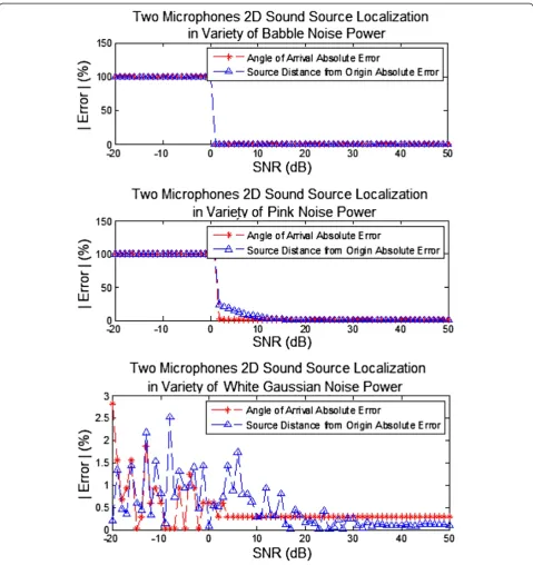
6. Simulations of TDE-ILD-based method and discussion
In order to use the introduced method for sound source localization in low reverberant outdoor cases, firstly we performed simulations. We tried to evaluate the accur-acy of this method in a variety of SNRs for some environ-mental noises. We considered two microphones onx-axis (y1=y2= 0) with 1-m distance from the origin (x1= 1m, x2=−1m (D = 2R = 2)) (Figure 1). In order to use PHAT for the calculation of time delay between the signals of the two microphones, we used a helicopter sound (wideband and quasi-periodic signal) with a length of approximately 4 s, downloaded from the internet (www.freesound.com) as our sound source. For different source locations and for an ambient temperature of 15°C, first we calculated sound speed in air using:
vsound¼20:05
ffiffiffiffiffiffiffiffiffiffiffiffiffiffiffiffiffiffiffiffiffiffiffiffiffiffiffiffiffiffiffiffiffiffiffiffiffiffiffiffiffiffiffiffiffiffiffiffiffiffiffiffiffiffiffiffiffiffiffiffiffiffiffiffiffiffiffiffiffiffi 273:15þTemperature Centigradeð Þ p
: ð61Þ
Then, we calculatedd1andd2using (24) and (25), and using (37), we calculated time delay between the re-ceived signals of the two microphones. For time delay positive values, i.e., sound source nearer to the first microphone (mic1 in Figure 1), we delayed second microphone signal with respect to the first microphone signal, and for negative values, i.e., sound source nearer to the second microphone (mic2 in Figure 1), did the opposite. Then using (6) and (7), we divided the first microphone signal by d1 and the second microphone signal by d2 to have correct attenuation in signals ac-cording to the source distances from microphones. Fi-nally, we tried to calculate source location using the proposed TDE-ILD method (Section 5) in a variety of SNRs for some environmental noises.
Assuming a high audio sampling rate, fractional delays are negligible and delays are rounded to nearest sampling point. Simulation results show larger localization error for SNRs lower than 10 dB. This issue occurs due to the use of ILD. Hence, we have to use this method for the case of only a dominant source to have accurate localization. Using spectral subtraction and source counting are useful for reducing localization error in SNRs lower than zero.
7. Our proposed TDE-ILD-HRTF method
Using TDE-ILD-based method, dual microphone 2D sound source localization is applicable. However, it is known that, by using a linear array in TDE-ILD-based method, two mirror points will be produced simultaneously (half-plane localization) [40]. Also, according to TDE-ILD-based simulation results (Section 6), it is noticeable that using ILD-based method needs only one dominant
high SNR source to be active in localization area. Our proposed TDE-ILD-HRTF method tries to solve these problems using source counting, noise reduction using spectral subtraction, and HRTF.
7.1. Source counting method
According to previous discussions, ILD-based method needs to use source counting to find that one dominant source is active for high-resolution localization. If more than one source is active in localization area, it cannot calculate m=E1/E2correctly. Therefore, we would need to count active and dominant sound sources and decide on localization of one sound source if only one source is dominant enough. PHAT gives us the cross-correlation vector of two microphone output signals. The number of dominant peaks of the cross-correlation vector gives us the number of dominant sound sources [66]. We consider only one source signal to be a periodic signal as:
s tð Þ ¼s tð þTÞ: ð62Þ
If the signals window is greater than T, calculating cross-correlation between the output signals of the two microphones gives us one dominant peak and some weak peaks with multiples of T distances. However, using signals window of approximately equal to T or using non-periodic source signal would lead to only one dominant peak when calculating cross-correlation be-tween the output signals of the two microphones. This peak value is delayed equal to the number of samples between the two microphones' output signals. Therefore, if one sound source is dominant in the localization area, only one dominant peak value will be in cross-correlation vector. Now, we consider having two sound sources s(t) and s'(t) in high SNR localization area. Ac-cording to (6) and (7), we have
s1ð Þ ¼t s tð−T1Þ þs0 t−T01
ð63Þ
s2ð Þ ¼t s tð−T2Þ þs0 t−T02
: ð64Þ
According to (32), we have
Rs1s2ð Þ ¼τ ∫þ−∞∞ s tð−T1Þ þs0 t−T01
ðs tð −T2þτÞ þs0
t−T02þτ
Þdt
ð65Þ
Rs1s2ð Þ ¼τ R1s1s2ð Þ þτ R2s1s2ð Þ þτ R3s1s2ð Þ þτ R4s1s2ð Þτ ð66Þ
where
R1s1s2ð Þ ¼τ ∫
þ∞
−∞ðt−T1Þ⋅s tð−T2þτÞdt ð67Þ
R2s1s2ð Þ ¼τ ∫
þ∞
−∞ðt−T1Þ⋅s0 t−T02þτ
dt ð68Þ
R3s1s2ð Þ ¼τ ∫
þ∞
−∞s0 t−T01
⋅s tð−T2þτÞdt ð69Þ
R4s1s2ð Þ ¼τ ∫
þ∞
−∞s0 t−T01
⋅s0 t−T02þτ
dt: ð70Þ
Using (34),τ1=T2−T1gives us a maximum value for R1s1s2ð Þτ ;τ2¼T02−T1, gives us a maximum value for R2s1s2ð Þτ ;τ3¼T2−T01, gives us a maximum value for R3s1s2ð Þτ andτ4¼T02−T01, and gives us a maximum value
for R4s1s2ð Þτ . Therefore, we will have four peak values in cross-correlation vector. However, according to this fact that (67) and (70) are cross-correlation functions of a sig-nal with delayed version of itself, and (68) and (69) are cross-correlation functions of two different signals,τ1and
τ4maximum values are dominant with respect toτ2andτ3 values. Now, we conclude in two dominant sound sources area, cross-correlation vector will have two dominant values and therefore equal count dominant values for more than two dominant sound sources signals as multiple power spectrum peaks in DOA-based multiple sound source beamforming methods [16]. Therefore, counting dominant cross-correlation vector values, we can find the number of active and dominant sound sources in localization area.
7.2. Noise reduction using spectral subtraction
In order to apply ILD in TDE-ILD-based dual microphone 2D sound source localization, source counting is used to find that one dominant high SNR source is active in localization area. Source counting was proposed to calcu-late the number of active sources in localization area. Fur-thermore, spectral subtraction can be used for noise reduction and therefore increasing active source's SNR. Also, according to the background noise, such as wind, rain, and babble, we can consider a background spectrum estimator. In the most practical cases, we can assume that the noisy signal can be modeled as the sum of the clean signal and the noise [67]:
snð Þ ¼t s tð Þ þn tð Þ: ð71Þ
Also according to this fact that the signal and noise are generated by independent sources, they are considered un-correlated. Therefore, the noisy spectrum can be written as:
Snð Þ ¼w S wð Þ þN wð Þ: ð72Þ
there can be used an adaptive background noise spectrum estimation procedure [67].
7.3. Using HRTF method
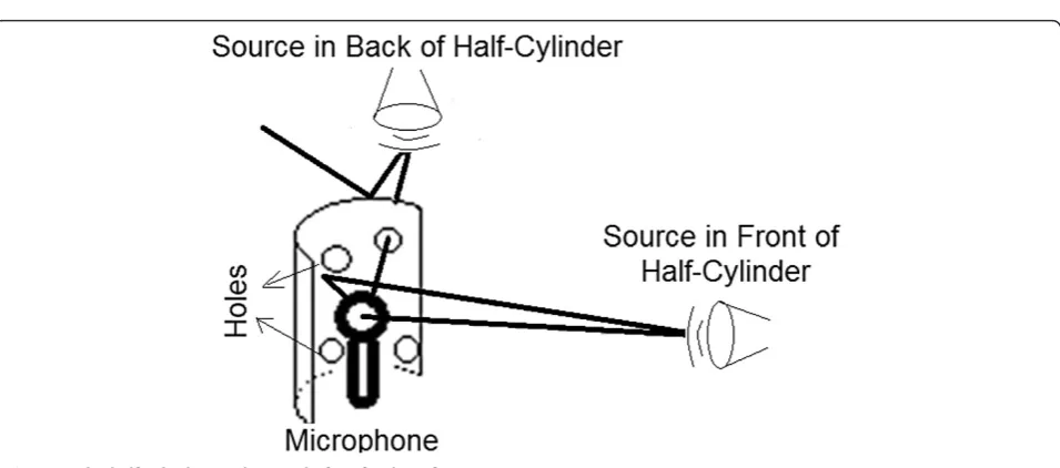
Using a linear array in TDE-ILD-based dual microphone 2D sound source localization method leads to two mir-ror points produced simultaneously. Adding an HRTF-inspired idea, whole-plane dual microphone 2D sound source localization would be possible. This idea was published in [68], and it is reviewed here again. Re-searchers have used an artificial ear with a spiral shape. This is a special type of pinna with a varying distance from a microphone placed in the center of its spiral [30]. However, we consider a half-cylinder instead of artificial ear [68]. Due to the use of such a reflector, a constant notch position is created for all variations (0 to180°) of sound signal angle of arrival (Figure 3). However, clearly, and as shown in the figure, a complete half-cylinder scatters the sound waves from sources behind it. In order to overcome this problem we consider slits on the surface of the half-cylinder (Figure 3). Ifdis the distance between the reflector (half-cylinder) and the microphone (placed at the center), a notch will be created when it is equal to quarter of the wavelength of sound,λ, plus any multiples of λ/2. For such wavelengths, the incident waves are reduced by reflected waves [30]:
n⋅ λ
2 þ
λ
4 ¼d n¼0;1;2;3:::: ð73Þ
These notches will appear at the following frequencies:
f ¼cλ¼ð2nþ1Þ:c
4d : ð74Þ
Covering only microphone 2 in Figure 1 by reflector, calculating the interaural spectral difference results in
ΔHð Þf
j j ¼10 log10H1ð Þf −10 log10H2ð Þf ¼ 10 log10H1ð Þf
H2ð Þf
: ð75Þ
High |ΔH(f)| values indicate that the sound source is in front, while negligible values indicate that sound source is at the back. One important point is that in order to have the same spectrum in both microphones when the sound source is at the back, careful design of the slits is necessary.
7.4. Extension of dimensions to three
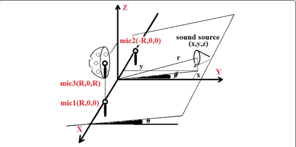
According to the use of half-cylinder reflector in the proposed localization system, this approach is only ap-plicable in 2D cases. Using a half-sphere reflector instead of the half-cylinder makes it usable in 3D sound source localization (Figure 4). Adding the half-sphere reflector only to microphone 2 in Figure 5 allows the localization system to localize sound sources in 3D cases.
For 3D case, we can consider a plane that passes through source position and x-axis and which makes an angle of θ with the x-y plane, and we name it source-plane (Figure 5). This source-plane consists of the microphones 1 and 2. According to these assumptions, using (36), we can calculate ф which is the angle of arrival in source-plane and is equal to angle of arrival inx-yplane. Then, using (59) and (60), we can also calculate xand y in 2D source-plane (not inx-yplane in 3D case) and therefore calculate sound source distance rpffiffiffiffiffiffiffiffiffiffiffiffiffiffiffix2þy2. Introducing
a new microphone (mic3 in Figure 5) withy= 0 andx=
z=R helps us calculate the angle θ. Therefore, using (36), we can calculateθas:
θ¼cos‐1 vsound⋅τ31
R
: ð76Þ
Using half-sphere reflector decreases accuracy of time delay and intensity level deference estimation between microphones 1 and 2 due to the change in the spectrum of second microphone's signal. However, covering the third microphone instead of the second microphone by half-sphere reflector only decreases the accuracy of time
delay estimation between the first and third micro-phones (Figure 5). Multiplying the inverse function of notch-filter in third microphone's spectrum leads to in-crease in accuracy. Now usingr,ф, andθ, we can calcu-late source locationx,yandzin 3D case:
x¼r:cosð Þϕ :sinð Þθ
y¼r:sinð Þϕ ;sinð Þθ
z¼r:cosð Þθ
:
8 <
: ð77Þ
The reasons for choosing the shape of sphere for the reflector are as follows [69]. The simplest type of
Figure 4Half-sphere used instead of artificial ear for 3D cases.
reflector is a plane reflector introduced to direct signal in a desired direction. Clearly, using this type of re-flector, the distance between reflector and microphone,
d in (73), varies with respect to source position in 3D cases leading to a change in notch position within spectrum. The change in notch position may not be suit-able as it might occur out of the spectral band of inter-est. To better adjust the energy in the forward direction, the geometrical shape of the plane reflector must be changed so as not to allow radiation in the back and side directions.
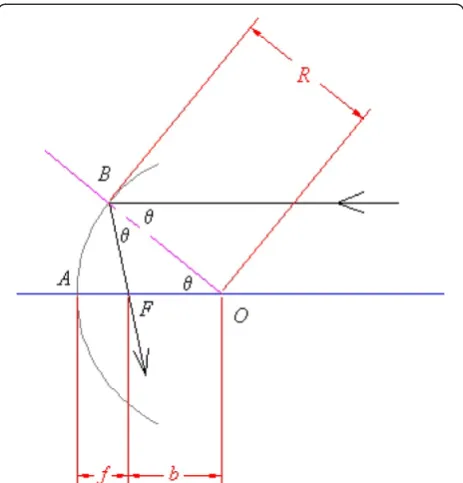
A possible arrangement for this purpose consists of two plane reflectors joined on one side to form a corner. This type of reflector returns the signal exactly in the same direction as it is received. Because of this unique feature, reflected wave acquired by the microphone is unique, which is our aim. Whereas having more than one reflected wave causes a higher energy value with re-spect to a single reflected wave at the microphone, which causes a deep notch. But using this type of re-flector,dis varied with respect to the source position in 3D cases which is related to notch position in spectrum. It has been shown that if a beam of parallel waves is in-cident upon a parabola reflector, the radiation will focus at a spot which is known as the focal point. This point in spherical reflector does not match to the center in ac-cordance with this fact that the center has equal distance (d) to all points of the reflector surface. Because of this feature, reflected wave which is received by the micro-phone is unique, whatever the position of the sound source, in 3D cases and belongs to the wave passing the center. The center of the spherical reflector with radius
Ris located atO(Figure 6). The sound wave axis strikes the reflector atB. From the Law of Reflection and angle geometry of parallel lines, the marked angles are equal. Hence, BFOis an equilateral triangle. Dropping the me-dian fromFwhich is stapled toBOand using trigonom-etry, the focal point is calculated as:
R
2b¼ cosð Þ→bθ ¼ R
2 cosθ ð78Þ
→F¼R− R
2 cosð Þθ : ð79Þ
Fis not equal to Rfor allθ values. The half-spherical reflector scatters the sound source waves hitting it from back. Therefore, we consider some slits on its surface (Figure 4). Obviously, the slits need to be designed in a fashion that leads to the same spectrum in both micro-phones when sound source is in back. When a plane wave hits a barrier with a single circular slit narrower than signal wavelength (λ), the wave bends and emerges from the slit as a circular wave [70]. If Lis the distance
between the slit and the viewing screen anddis the slit width, based on the assumption that L> >d(Fraunhofer scattering), the wave intensity distribution observed (on a screen) at an angleθ with respect to the incident dir-ection is given by:
if k¼πλ:d sinð Þ→θ Ið Þθ
Ið Þθ ¼
sin2ð Þk
k2 ; ð80Þ
where I(θ) is wave intensity in direction of observation and I(0) is maximum wave intensity of diffraction pat-tern (central fringe). This relationship will have a value of zero each time sin2(k) = 0. This occurs when
k¼ mπorπ:d
λ sinð Þ ¼ mθ π; ð81Þ
yielding the following condition for observing minimum wave intensity from a single circular slit:
sinð Þ ¼θ mλ
d m¼0;2; :::: ð82Þ
This relationship is satisfied for integer values of m. Increasing values of mgives minima at correspondingly larger angles. The first minimum will be found form= 1, the second form= 2, and so forth. If d
λsinð Þθ is less than one for all values ofθ, i.e., when the size of the aperture is smaller than a wavelength (d<λ), there will be no minima. As we need more than one circular slit on half-sphere reflector's surface, we consider a parallel wave incident on a barrier that consists of two closely spaced narrow
circular slits S1 and S2. The narrow circular slits split the incident wave into two coherent waves. After passing through the slits, the two waves spread out due to dif-fraction interfere with one another. If this transmitted wave is made to fall on a screen some distance away, an interference pattern of bright and dark fringes are ob-served on the screen, with the bright ones corresponding to regions of maximum wave intensity while the dark ones corresponding to those of minimum wave intensity. As discussed before, for all points on the screen where the path difference is some integer multiple of the wave-length, the two waves from the slits S1 and S2 arrive in phase and bright fringes are observed. Thus, the condi-tion for producing bright fringes is as in (82). Similarly, dark fringes are produced on the screen if the two waves arriving on the screen from slits S1 and S2 are exactly out of phase. This happens if the path difference be-tween the two waves is an odd integer multiple of half-wavelengths:
sinð Þ ¼θ mþ
1 2
:λ
d m¼0;1;2; :::: ð83Þ
Of course, this condition is changed using a half-sphere instead of a plane (Figure 7), where according to the same distance R to the center, the two waves from the slits S1 and S2 arrive in phase at the center and bright fringes are observed there. This signal intensity magnification is not suitable for the case of estimating intensity level difference between two microphones where one of them is covered by this reflector. However, covering the third microphone by half-sphere reflector is suitable where there is no need to estimate the intensity level difference between two microphones 1 and 3.
8. TDE-ILD-HRTF approach algorithm
According to previous discussions, the following steps can be considered for our proposed method:
1. Setup microphones and hardware.
2. Calculate the sound recording hardware set (microphone, preamplifier, and sound card) amplification normalizing factor.
3. Apply voice activity detection. Is there valuable signal? yes→go to 4 no→go to 3.
4. Obtains1(t),s2(t), ands3(t)→m=E1/E2.
5. Remove DC from the signals. Then normalize them regarding the sound intensity.
6. Hamming window signals regarding their stationary parts (at least about 100 ms for wideband quasi-periodic helicopter sound or twice that). 7. Apply FFT to signals.
8. Cancel noise using spectral subtraction.
9. Apply PHAT to the signals in order to calculateτ21
andτ31in frequency domain (index of first
maximum value). Then find the second maximum value of cross-correlation vector.
10. If the first maximum value is not dominant enough with respect to the second maximum value, go to the next windows of signals and do not calculate sound source location, otherwise:
a.
Φ¼cos−1 vsound:τ21
2R
andθ¼cos−1 vsound:τ31
R
b.
vsound¼20:05
ffiffiffiffiffiffiffiffiffiffiffiffiffiffiffiffiffiffiffiffiffiffiffiffiffiffiffiffiffiffiffiffiffiffiffiffiffiffiffiffiffiffiffiffiffiffiffiffiffiffiffiffiffiffiffiffiffiffiffiffiffiffiffiffiffiffiffiffiffiffi 273:15þTemperature Centigradeð Þ p
c.
r1¼τ21:vsound
1−pffiffiffiffim andr2¼
τ21:vsound:pffiffiffiffim
1−pffiffiffiffim
d.
x¼ r2 2−r21
=4Randy¼
ffiffiffiffiffiffiffiffiffiffiffiffiffiffiffiffiffiffiffiffiffi r2
1−ðx−RÞ 2
q
e.
ΔHð Þf
j j ¼ 10log10H1ð Þf
H3ð Þf
f.
ifðjΔHð Þf j≈0Þy¼−
ffiffiffiffiffiffiffiffiffiffiffiffiffiffiffiffiffiffiffiffiffi r2
1−ðx−RÞ 2
q
elsey¼
ffiffiffiffiffiffiffiffiffiffiffiffiffiffiffiffiffiffiffiffiffi
r2 1−ðx−RÞ
2
q
→ xyss¼¼rr::cossinð Þð ÞΦΦ::sinsinð Þð Þθθ
zs¼r:cosð Þθ
8 < :
g. Go to 3.
9. Hardware and software implementations and results
We implemented our proposed hardware using‘MB800H’ motherboard and DELTA IOIO LT sound card from M-Audio featuring eight analogue sound inputs, 96-kHz sampling frequency, and up to 16-bit resolution. Three MicroMic microphones of type ‘C 417’ with B29L pre-amplifier were used for the implementation (Figure 8). The reason for using this type of microphone is its very
flat spectral response up to 5 kHz. Visual C++ used for software implementation. According to the very low sensi-tivity of the used microphones (10 mV/Pa), a loudspeaker was used for the sound source. Initially, we used micro-phones one and two to evaluate the accuracy of the angle of arrival ф as well as microphones one and three to evaluate the accuracy of the angle of arrivalθ. We consid-ered 1 m(R=D/2 = 1) distance between every microphone and the origin. Sound localization results showed that sound velocity changed in different temperatures. Since the sound velocity was used in most of the steps of the proposed methods, sound source location calculations were carried out inaccurately. Therefore, (61) was used based on a thermometer reading in order to more
Figure 8Setup of the proposed 3D sound source localization method using four microphones.
Table 1 Results of the azimuth angle of arrival based on hardware implementation
фReal angle (degrees)
фProposed method results for angle of arrival (degrees)
Absolute value of error (degrees)
0 0.18 0.18
15 15.13 0.13
30 29.85 0.15
45 45.18 0.18
60 60.14 0.14
75 74.91 0.09
90 89.83 0.17
105 104.82 0.18
120 120.14 0.14
135 135.11 0.11
150 150.14 0.14
165 165.09 0.09
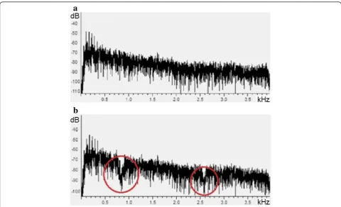
accurately find the sound velocity in different tempera-tures. Angle of arrival calculations using downloaded wideband quasi-periodic helicopter sound resulted in Tables 1 and 2. Acquisition hardware was initialized to 96-kHz sampling frequency and 16-bit resolution. Also signal acquisition window length was set to 100 ms. A custom 2-cm-diameter reflector (Figure 8) was placed behind the third microphone. Using the aforementioned sound source, the sound spectra shown in Figure 9 were measured using the third microphone. Figure 9a shows the spectrum when
the sound source has been placed behind the reflector and Figure 9b when placed in front of it. Notches can be spot-ted in the second spectrum according to the reflector diameter and (74). Finally, using our proposed TDE-ILD-HRTF approach, first we tried to find that a dominant source is active in localization area. Then, using (72), we tried to reduce background noise and localize sound source in 3D space. Table 3 shows the improved results after the application of noise reduction method. Although PHAT features high performance in noisy and reflective environments, due to the rather constant and high valued signal-to-reverberation ratio (SRR) in outdoor cases, this feature could not be evaluated. We tried to find the effect of probable reverberation on our localization system re-sults. In order to alleviate reverberation, our experiments indicated that at least a distance of 1.2 m with surround-ing buildsurround-ings would be necessary. Although the loudspea-ker's power, the hardware set (microphone, preamplifier, and sound card) amplification factor and the distance of the microphones with the surrounding buildings indicate the SNR value for reverberate signals in a real environ-ment, this distance can be calculated, but it can also be in-dicated experimentally, which is easier. Tables 1 and 2 indicate that our implemented 3D sound source localiza-tion method features less than 0.2 degree error for angle of arrival. Table 3 indicates less than 10% error for 3D Table 2 Results of the elevation angle of arrival based on
hardware implementation
θReal angle
(degrees) θ
Proposed method results for angle of arrival (degrees)
Absolute value of error (degrees)
−10 −10.18 0.18
−5 −5.16 0.16
0 0.05 0.05
15 14.15 0.15
30 29.91 0.09
45 45.19 0.19
60 60.13 0.13
75 75.11 0.11
90 89.82 0.18
location finding. It also indicates ambiguity in sign finding between 0.5° and−0.5° as well as 175° and 185° due to the implemented reflector edges. We measured processing times of less than 150 ms for every location calculation. Comparing angle of arrival results with the results re-ported in various cited papers, the best rere-ported results (on approximately similar tasks) were 1 degree limit error in [71], 2 degree limit error in [72], and within 8 degree error in [73]. Note that the fundamental limit of bearing estimates determined by Cramer-Rao Lower Bound (CRLB) forD= 1 cm spacing of the microphone pair, sam-pling frequency of 25 kHz and estimation duration of 100 ms, is computed to be 1° [71]. This is found equal to 1.4° for our system. However, only few respectable refer-ences have calculated 2D or 3D source locations accur-ately. Most of such research reports, besides calculating
the angle of arrival, used either least-square error estima-tion or Kalman filtering techniques to predict moestima-tion path of sound sources, in order to overcome their local calcula-tion errors. Examples are [2], [13], [15], and [19]. Mean-while, comparison of our results with these and other works (results on approximately similar tasks), such as [72] and [73], shows the approximately same accuracy na-ture of our proposed source location measurement approach.
10. Conclusion
In this paper, we reported on the simulation of TDE-ILD-based 2D half-plane sound source localization using only two microphones. Reduction of the microphone count was our goal. Therefore, we also proposed and implemented TDE-ILD-HRTF-based 3D entire-space sound Table 3 Results for proposed 3D sound source localization method (Section 7) using noise reduction procedure
Real location (m) Proposed method results (m) Absolute error (m)
x y z x y z x y z
1 10 5 1.9 9.2 4.1 0.9 0.8 0.9
2 10 5 2.9 9.2 4.3 0.9 0.8 0.7
3 10 5 2.2 10.7 5.6 0.8 0.7 0.6
4 10 5 3.2 10.7 5.8 0.8 0.7 0.8
5 10 5 5.5 9.5 5.8 0.5 0.5 0.8
6 10 5 6.5 10.5 4.5 0.5 0.5 0.5
7 10 5 7.7 10.8 4.4 0.7 0.8 0.6
8 10 5 8.6 10.8 4.4 0.6 0.8 0.6
9 10 5 9.8 9.1 4.2 0.8 0.9 0.8
10 10 5 9.5 9.4 5.9 0.5 0.6 0.9
10 15 5 10.6 15.7 5.5 0.6 0.7 0.5
10 20 5 10.7 19.2 5.6 0.7 0.8 0.6
10 25 5 9.2 23.9 5.7 0.8 1.1 0.7
10 30 5 10.5 31.7 4.3 0.5 1.7 0.7
10 9 5 10.8 9.7 5.8 0.8 0.7 0.8
10 8 5 9.3 8.7 5.8 0.7 0.7 0.8
10 1 5 10.6 6.5 5.9 0.6 0.5 0.9
10 6 5 9.5 6.6 4.1 0.5 0.6 0.9
10 5 5 10.5 4.5 4.2 0.5 0.5 0.8
10 4 5 10.6 3.4 5.7 0.6 0.6 0.7
10 3 5 9.3 3.6 5.5 0.7 0.6 0.5
10 2 5 10.8 ±2.8 5.8 0.8 0.8 0.8
10 1 5 10.1 ±0.2 4.3 0.1 0.8 0.7
10 −1 5 10.6 ±0.4 4.1 0.6 0.6 0.9
10 −2 5 10.5 ±2.7 5.6 0.5 0.7 0.6
10 −3 5 10.4 −2.8 5.5 0.4 0.2 0.5
10 −4 5 9.7 −3.7 5.5 0.3 0.3 0.5
source localization using only three microphones. Also, we used spectral subtraction and source counting methods in low-degree reverberation outdoor cases to increase localization accuracy. According to Table 3, implemen-tation results show that the proposed method has led to less than 10% error for 3D location finding. This is a higher accuracy in source location measurement in comparison with similar researches which did not use spectral subtraction and source counting. Also, we indi-cated that partly covering one of the microphones by a half-sphere reflector leads to entire-space N-dimensional sound source localization using onlyN-microphones.
Competing interests
The authors declare that they have no competing interests.
Authors’information
AP was born in Azerbaijan. He has a Ph.D. in Electrical Engineering (Signal Processing) from the Electrical Engineering Department, Amirkabir University of Technology, Tehran, Iran. He is now an invited lecturer at the Electrical Engineering Department, Amirkabir University of Technology and has been teaching several courses (C++ programming, multimedia systems, digital signal processing, digital audio processing, and digital image processing). His research interests include statistical signal processing and applications, digital signal processing and applications, digital audio processing and applications (acoustic modeling, speech coding, text to speech, audio watermarking and steganography, sound source localization, determined and underdetermined blind source separation and scene analyzing), digital image processing and applications (image and video coding, image watermarking and
steganography, video watermarking and steganography, object tracking and scene matching) as well as BCI.
SMA received his B.S. and M.S. degrees in Electronics from the Electrical Engineering Department, Amirkabir University of Technology, Tehran, Iran, in 1984 and 1987, respectively, and his Ph.D. in Engineering from the University of Cambridge, Cambridge, U.K., in 1996, in the field of speech processing. Since 1988, he has been a Faculty Member at the Electrical Engineering Department, Amirkabir University of Technology, where he is currently an associate professor and teaches several courses and conducts research in electronics and communications. His research interests include speech processing, acoustic modeling, robust speech recognition, speaker adaptation, speech enhancement as well as audio and speech watermarking.
Received: 24 June 2013 Accepted: 21 November 2013 Published: 6 December 2013
References
1. GC Carter, Time delay estimation for passive sonar signal processing. IEEE T Acoust S.ASSP-29, 462–470 (1981)
2. E Weinstein, Optimal source localization and tracking from passive array measurements. IEEE T. Acoust. S.ASSP-30, 69–76 (1982)
3. H Wang, P Chu,Voice source localization for automatic camera pointing system in videoconferencing, in Proceedings of the ICASSP, New Paltz, NY, 19–22, 1997
4. J Caffery Jr, G Stüber, Subscriber location in CDMA cellular networks. IEEE Trans. Veh. Technol.47, 406–416 (1998)
5. JB Tsui,Fundamentals of Global Positioning System Receivers(Wiley, New York, 2000)
6. F Klein,Finding an earthquake's location with modern seismic networks (Earthquake Hazards Program, Northern California, 2000)
7. Y Huang, J Benesty, GW Elko, RM Mersereau, Real-time passive source localization: A practical linear-correction least-squares approach. IEEE T. Audio P.9, 943–956 (2001)
8. VJM Michaud, F Rouat, J Letourneau,Robust Sound Source Localization Using a Microphone Array on a Mobile Robot(in Proceedings of the IEEE/RSJ International Conference on Intelligent Robots and Systems, vol. 2, Las Vegas), pp. 1228–1233
9. BLF Daku, JE Salt, L Sha, AF Prugger, An algorithm for locating microseismic events, inProceedings of the IEEE Canadian Conference on Electrical and Computer Engineering. Niagara Falls.2–5, 2311–2314 (May 2004) 10. N Patwari, JN Ash, S Kyperountas, AO Hero III, RL Moses, NS Correal,
Locating the nodes. IEEE Signal Process. Mag.22, 54–69 (2005) 11. S Gezici, T Zhi, G Giannakis, H Kobayashi, A Molisch, H Poor, Z Sahinoglu,
Localization via ultra-wideband radios: a look at positioning aspects for future sensor networks. IEEE Signal Process. Mag.22, 70–84 (2005) 12. JY Lee, SY Ji, M Hahn, C Young-Jo,Real-Time Sound Localization Using Time
Difference for Human-Robot Interaction(in Proceedings of the 16th IFAC World Congress, Prague, 2005)
13. WK Ma, BN Vo, SS Singh, A Baddeley, Tracking an unknown time-varying number of speakers using TDOA measurements: a random finite set approach. IEEE Trans. Signal. Process.54(9), 3291–3304 (2006) 14. KC Ho, X Lu, L Kovavisaruch, Source localization using TDOA and FDOA
measurements in the presence of receiver location errors: analysis and solution. IEEE Trans Signal. Process.55(2), 684–696 (2007)
15. V Cevher, AC Sankaranarayanan, JH McClellan, R Chellappa, Target tracking using a joint acoustic video system. IEEE Trans. Multimedia.9(4), 715–727 (2007) 16. X Zhengyuan, N Liu, BM Sadler,A Simple Closed-Form Linear Source
Localization Algorithm(in IEEE MILCOM, Orlando, FL, 2007), pp. 1–7 17. JPV Etten, Navigation systems: fundamentals of low and very-low frequency
hyperbolic techniques. Elec. Comm.45(3), 192–212 (1970)
18. RO Schmidt, A new approach to geometry of range difference location. IEEE Trans. Aerosp. Electron Syst.AES-8(6), 821–835 (1972)
19. HB Lee, A novel procedure for assessing the accuracy of hyperbolic multilateration systems. IEEE Trans. Aerosp. Electron Syst.110(1), 2–15 (1975) 20. WR Hahn, Optimum signal processing for passive sonar range and bearing
estimation. J. Acoust. Soc. Am.58, 201–207 (1975)
21. P Julian, A Comparative, Study of Sound Localization Algorithms for Energy Aware Sensor Network Nodes. IEEE Trans. Circuits and Systems - I. 51(4) (2004)
22. ST Birchfield, R Gangishetty,Acoustic Localization by Interaural Level Difference (in Proceedings of the ICASSP, Philadelphia, PA, 2005), pp. 1109–1112 23. KC Ho, M Sun, An accurate algebraic Closed-Form solution for energy-based
source localization. IEEE Trans. Audio, Speech. Lang. Process 15, 2542–2550 (2007)
24. KC Ho, M Sun, Passive Source Localization Using Time Differences of Arrival and Gain Ratios of Arrival. IEEE Trans. Signal. Process56, 2 (2008) 25. JH Hebrank, D Wright, Spectral cues used in the localization of sound
sources on the median plane. J. Acoust. Soc. Am.56, 1829–1834 (1974) 26. JC Middlebrooks, JC Makous, DM Green, Directional sensitivity of
sound-pressure level in the human ear canal. J Acoust Soc Am.1, 86 (1989) 27. F Asano, Y Suzuki, T Sone, Role of spectral cues in median plane
localization. J. Acoust. Soc. Am.88, 159–168 (1990)
28. RO Duda, WL Martens, Range dependence of the response of a spherical head model. J. Acoust. Soc. Am.104(5), 3048–3058 (1998)
29. CI Cheng, GH Wakefield, Introduction to head-related transfer functions (HRTFS): representations of HRTFs in time, frequency, and space. J. of the Audio Engin. Soc.49(4), 231–248 (2001)
30. A Kulaib, M Al-Mualla, D Vernon,2D Binaural Sound Localization for Urban Search and Rescue Robotic. inProceedings of the 12th Int(Conference on Climbing and Walking Robots, Istanbul, 2009), pp. 9–11
31. S Razin, Explicit (non-iterative) Loran solution. J. Inst. Navigation14(3) (1967) 32. C Knapp, G Carter, The generalized correlation method for estimation of
time delay. IEEE Trans. Acoust., Speech. Signal Process.ASSP-24(4), 320–327 (1976)
33. MS Brandstein, H Silverman, A practical methodology for speech localization with microphone arrays. Comput Speech Lang.11(2), 91–126 (1997) 34. MS Brandstein, JE Adcock, HF Silverman, A Closed-Form location estimator
for use with room environment microphone arrays. IEEE Trans. Speech Audio Process.5(1), 45–50 (1997)
35. P Svnizer, M Matnssoni, M Omologo,Acoustic Source Location in a THREE-Dimensional Space Using Crosspower Spectrum Phase(in Proceedings of the ICASSP, Munich, 1997), p. 231
36. E Lleida, J Fernandez, E Masgrau,Robust continuous speech recog. sys. based on a microphone array(in Proceedings of the ICASSP, Seattle, WA, 1998), pp. 241–244
38. M Omologo, P Svaizer,Acoustic Event Localization using a Crosspower-Spectrum Phase based Technique(in Proceedings of the ICASSP, vol. 2, Adelaide, 1994), pp. 273–276
39. C Zhang, D Florencio, Z Zhang,Why Does PHAT Work Well in Low Noise, reverberative Environments(in Proceedings of the ICASSP, Las Vegas, NV, 2008), pp. 2565–2568
40. W Cui, Z Cao, J Wei,DUAL-Microphone Source Location Method in 2-D Space (in Proceedings of the ICASSP, Toulouse, 2006), pp. 845–848
41. X Sheng, YH Hu, Maximum likelihood multiple-source localization using acoustic energy measurements with wireless sensor networks. IEEE Trans Signal Process53(1), 44–53 (2005)
42. D Blatt, AD Hero III, Energy-based sensor network source localization via projection onto convex sets. IEEE Trans Signal Process54(9), 3614–3619 (2006)
43. S Sen, A Nehorai, Performance analysis of 3-D direction estimation based on head-related transfer function. IEEE Trans. Audio Speech Lang. Process 17(4) (2009)
44. DW Batteau, The role of the pinna in human localization. Series B, Biol. Sci 168, 158–180 (1967)
45. SK Roffler, RA Butler, Factors that influence the localization of sound in the vertical plane. J. Acoust. Soc. Am.43(6), 1255–1259 (1968)
46. SR Oldfield, SPA Parker, Acuity of sound localization: a topography of auditory space. Perception13(5), 601–617 (1984)
47. PM Hofman, JGAV Riswick, AJV Opstal, Relearing sound localization with new ears. Nature Neurosci.1(5), 417–421 (1998)
48. CP Brown,Modeling the Elevation Characteristics of the Head-Related Impulse Response(San Jose State University, San Jose, CA, M.S. Thesis, 1996) 49. P Satarzadeh, VR Algazi, RO Duda,Physical and filter pinna models based on
anthropometry(in Proceedings of the 122nd Conv, Audio Eng. Soc, Vienna, 2007), p. 7098
50. S Hwang, Y Park, Y Park,Sound Source Localization using HRTF database (in ICCAS2005, Gyeonggi-Do, 2005)
51. WH Foy, Position-location solution by Taylor-series estimation. IEEE Trans. Aerosp. Electron Syst.AES-12, 187–194 (1976)
52. JS Abel, JO Smith, Source range and depth estimation from multipath range difference measurements. IEEE Trans. Acoust. Speech. Signal. Process. 37, 1157–1165 (1989)
53. DMY Sommerville,Elements of Non-Euclidean Geometry(Dover, New York, 1958). pp. 260–1958
54. LP Eisenhart,A Treatise on the Differential Geometry of Curves and Surfaces (New York, Dover, 1960), pp. 270–271. originally Ginn, 1909
55. JO Smith, JS Abel, Closed-Form least-squares source location estimation from range-difference measurements. IEEE Trans. Acoust. Speech Signal Process.ASSP-35, 1661–1669 (1987)
56. JM Delosme, M Morf, B Friedlander,A linear equation approach to locating sources from time-difference-of-arrival measurements(in Proceedings of the ICASSP, Denver, CO, 1980), pp. 09–11
57. BT Fang, Simple solutions for hyperbolic and related position fixes. IEEE Trans. Aerosp. Electron Syst.26, 748–753 (1990)
58. B Friedlander, A passive localization algorithm and its accuracy analysis. IEEE J. Oceanic Eng.OE-12, 234–245 (1987)
59. HC Schau, AZ Robinson, Passive source localization employing intersecting spherical surfaces from time-of-arrival differences. IEEE Trans. Acoust. Speech Signal Process.ASSP-35, 1223–1225 (1987)
60. JS Abel, A divide and conquer approach to least-squares estimation. IEEE Trans. Aerosp. Electron. Syst.26, 423–427 (1990)
61. A Beck, P Stoica, J Li, Exact and approximate solutions of source localization problems. IEEE Trans. Signal. Process.56(5), 1770–1778 (2008)
62. HC So, YT Chan, FKW Chan, Closed-Form Formulae for Time-Difference-of-Arrival Estimation. IEEE Trans Signal Process56, 6 (2008)
63. MD Gillette, HF Silverman, A linear closed-form algorithm for source localization from time-differences of arrival. IEEE Signal Process. Lett. 15, 1–4 (2008)
64. EG Larsson, D Danev, Accuracy comparison of LS and squared-range ls for source localization. IEEE Trans. Signal. Process58, 2 (2010)
65. N Ono, S Sagayama, R-means localization: a simple iterative algorithm for range-difference-based source localization. in Proceedings of the ICASSP. 14–19, 2718–2721 (March 2010)
66. ZE Chami, A Guerin, A Pham, C Servière,A PHASE-based Dual Microphone Method to Count and Locate Audio Sources in Reverberant Rooms(in IEEE
Workshop on Applications of Signal Processing to Audio and Acoustics, New Paltz, NY, 2000), pp. 18–21
67. SV Vaseghi,Advanced Digital Signal Processing and Noise Reduction(3rd edn, John Wiley & Sons, Ltd, Hoboken, NJ, 2006)
68. A Pourmohammad, SM Ahadi, TDE-ILD-HRTF-based 2D whole-plane sound source localization using only two microphones and source counting. Int. J. Info. Eng.2(3), 307–313 (2012)
69. CA Balanis,Antenna Theory: Analysis and Design (John Wiley & Sons Inc(NJ, Hoboken, 2005)
70. DC Giancoli,Physics for Scientists and Engineers, vol. I (Upper Saddle River, Prentice Hall, 2000)
71. B Friedlander, On the Cramer-Rao bound for time delay and Doppler estimation. IEEE Trans. Inf. Theory.30(3), 575–580 (1984)
72. A Gore, A Fazel, S Chakrabartty, Far-Field Acoustic Source Localization and Bearing Estimation Using∑ΔLearners. IEEE Trans. circuits and systems-I: regular papers57(4) (2010)
73. SH Chen, JF Wang, MH Chen, ZW Sun, MJ Liao, SC Lin, SJ Chang,A Design of Far-Field Speaker Localization System using Independent Component Analysis with Subspace Speech Enhancement(in Proc. 11th IEEE Int. Symp. Mult., San Diego, CA, 2009), pp. 14–16
doi:10.1186/1687-4722-2013-27
Cite this article as:Pourmohammad and Ahadi:N-dimensionalN -microphone sound source localization.EURASIP Journal on Audio, Speech, and Music Processing20132013:27.
Submit your manuscript to a
journal and benefi t from:
7Convenient online submission
7Rigorous peer review
7Immediate publication on acceptance
7Open access: articles freely available online
7High visibility within the fi eld
7Retaining the copyright to your article