R E S E A R C H A R T I C L E
Open Access
Coupled domain decomposition–proper
orthogonal decomposition methods for
the simulation of quasi-brittle fracture
processes
Alberto Corigliano
∗, Federica Confalonieri, Martino Dossi and Stefano Mariani
*Correspondence:
[email protected] Department of Civil and Environmental Engineering, Politecnico di Milano, Piazza Leonardo da Vinci, 32, 20133 Milano, Italy
Abstract
In this paper, we discuss a strategy to reduce the computational costs of the simulation of dynamic fracture processes in quasi-brittle materials, based on a combination of domain decomposition (DD) and model order reduction (MOR) techniques. Fracture processes are simulated by means of three-dimensional finite element models in which use is made of cohesive elements, introduced on-the-fly wherever a cracking criterion is attained. The body is initially subdivided into sub-domains; for each sub-domain MOR is obtained through a proper orthogonal decomposition (POD) of the equations governing its evolution, until when it starts getting cracked. After crack inception within a sub-domain, the solution is switched back to the original full-order model for that sub-domain only. The computational gain attained through the coupled use of DD and POD thus depends on the geometry of the body, on the topology of sub-domains and, on top of all, on the spreading of cracking induced by load conditions. Numerical examples concerning well-established fracture tests are used for validation, and the attainable reduction of the computing time is discussed at varying decomposition into sub-domains, even in the absence of a full exploitation of parallel computing
potentialities.
Keywords: Quasi-brittle fracture, Domain decomposition, Model order reduction (MOR), Proper orthogonal decomposition (POD)
Background
One of the most active sectors in computational mechanics looks for more and more efficient strategies for the highly realistic simulation of complex phenomena. Two main driving forces guide these researches. The first one is the attempt to simulate phenomena in an extremely fast way, possibly reaching real-time computing; recent contributions in this field are e.g. [1,2]. The second strong motivation is the attempt to perform simulations that with standard strategies would simply be practically impossible due to unacceptable computing times; examples in this line are those of [3–5].
Domain decomposition (DD) and model order reduction (MOR) approaches are typical tools developed to reach the above goals, not only in the field of computational mechanics but more generally in the extremely vast field of computational sciences. Proper
orthogo-©The Author(s) 2016. This article is distributed under the terms of the Creative Commons Attribution 4.0 International License (http://creativecommons.org/licenses/by/4.0/), which permits unrestricted use, distribution, and reproduction in any medium, provided you give appropriate credit to the original author(s) and the source, provide a link to the Creative Commons license, and indicate if changes were made.
nal decomposition (POD), see e.g. [6], is a MOR strategy that has recently received much attention as a tool to drastically reduce the number of degrees of freedom (DOFs) retained in an analysis, being extremely efficient in linear problems. Many difficulties arise when trying to apply POD to non-linear, irreversible problems; various strategies have been recently developed to this purpose, among these e.g. the so-called proper generalized decomposition (PGD) originally proposed by Ladevèze with a different terminology and recently applied e.g. in [7–10].
The purpose of this paper is to further contribute to a series of works recently published by the Authors on the efficient application of DD and MOR-POD techniques to multi-physics and non-linear, irreversible problems. DD methods, based on an extension of the algorithm originally proposed in [11], were applied to the solution of the electro-mechanical coupled problem in microsystems in [12], and to the simulation of quasi brittle fracture processes in [13]. A combination of DD and MOR-POD techniques was proposed in [14] for the electro-mechanical coupled problem in microsystems and in [15] for the solution of elasto-plastic dynamic problems.
Moving from the aforementioned implementation in [15], we address here the prob-lem of dynamic propagation of cohesive cracks in a quasi-brittle material. Although the spreading of dissipative phenomena can be rather different in elasto-plasticity and quasi-brittle cracking, especially when the solution is dominated in the latter case by the growth of a dominant crack, the two problems can be approached in a similar way as far as MOR is concerned. The coupled DD-POD approach here adopted is therefore similar to the one proposed in [15]: the whole body is initially subdivided in sub-domains; for each sub-domain, a reduced-order model is trained in the initial stage of the analysis; as soon as a sub-domain starts being cracked, the relevant solution is switched back to the original full-order model and then advanced in time. The handling of each sub-domain through an either reduced- or full-order mode can be therefore optimally approached via an heterogeneous time integration procedure, see [13].
The proposed approach reaches a good compromise between the contrasting needs of realistically reproducing complex fracture processes in possibly highly heterogeneous materials, and of being able to keep under acceptable levels the computing time.
The paper is organized in three main sections in addition to the “Introduction” and “Conclusion” sections. First, the semi-discretized problem formulation for an elastic body containing cohesive fracture process zones, in the presence of dynamic loading is discussed and presented. In the central main section the proposed new computational strategy is described in details. The third main section is devoted to the critical discussion of num erical examples.
Throughout the paper, a matrix Voigt notation is adopted.
Problem formulation
Fig. 1 Reference cracking continuum: notation
CTσ+b=ρu¨ in \
c; (1a)
Nσ=f on f; (1b)
Mσ= −τ+ on +
c, Mσ=τ− on −c. (1c)
Here:c+andc−are the two sides ofc, acted by tractionsτ+andτ−in the cohesive region of the crack surface;ρis the mass density;σis the vector gathering the independent components of the stress tensor; C is the differential compatibility operator; ¨u is the acceleration vector;N andMare matrices collecting the components of vectorsnand m, respectively;nis the unit outward normal vector to;mis the unit vector normal toc, pointing towards side+c of the crack (whichever it is, see [16]). The equilibrium condition acrosscalso provides:
τ≡τ−= −τ+ on
c. (2)
Compatibility in the bulk\cis given by:
ε=Cu in \c, (3)
ε being the vector gathering the independent components of the strain tensor, and u the displacement vector. The displacement discontinuity [u] acrosscis instead given in terms of the displacement field on the two sides of the discontinuity, according to:
[u]=u+
c −u−c. (4)
For quasi-brittle materials, a cohesive law is introduced to model the decohesion between the two sides of the crack c, i.e. the interaction between the sides in case of crack opening/sliding (avoiding for the time being the possible frictional contact in case of crack closure). We then state, see [17–20]:
τ=τ([u],ψ) on c, (5)
The governing equations are completed by the initial conditions in terms of displace-ment and velocity fields.
Assuming material damping to be null, dynamic equilibrium can be written in weak form as [16]:
ρδu
Tu¨ d+
δε
Tσ d+
c
δ[u]Tτd=
δu
Tb d+
f
δuTfd
∀δus.t.δu=0 on u, δε=Cδu in \c, (6)
where u needs to be a continuously differentiable field in the bulk of the body \c, possibly displaying jumps across the crackc.
Moving to the semi-discretized finite element formulation, the approximate displace-ment, displacement jump and deformation vectors can be written as [21,22]:
u∼=NU; (7a)
[u]∼=BU; (7b)
ε∼=CNU=BU, (7c)
whereUis the nodal displacement vector;Nis the matrix of nodal shape functions;B andBare the matrices respectively representing compatibility along the crack and in the bulk. The weak formulation (6), upon assembling over the entire domain, can be written as:
MU¨ +F(U)+F(U)=F, (8)
and have to be supplemented by initial conditions on the displacement and the velocity vectors. In Eq. (8):Mis the symmetric, positive-definite mass matrix;FandFare the vectors of internal forces due to bulk and cohesive contributions; andFis the vector of external loads. They respectively read:
M=
ρN
TN
d, (9a)
F=
B
T
σd, (9b)
F=
c
BTτd, (9c)
F=
N
Tb d+
f
NTfd. (9d)
Cohesive methodologies have been widely employed within the finite element framework for the simulation of fracture processes in quasi brittle materials, either through the inter-element technique, i.e. assuming the propagation to occur only along the element faces [13,20,23–29], or combined with extended approaches to allow for intra-element propagation [16,30–32].
char-acteristic element size to be smaller than a material length-scale, which in accordance with Irwin’s estimation reads [36]:
= EG τ2
max,
(10)
where:E is the material Young’s modulus, whileGandτmax respectively stand for its
fracture energy and tensile strength.
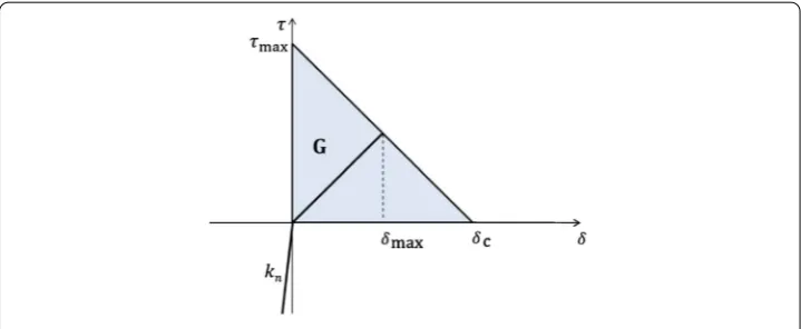
The adopted cohesive model consists in a softening law linking the tractions acting on the crack surfaces to the displacement jump. Following [25,26], this cohesive law is given in terms of effective displacement jumpδand effective tractionτ, see Fig.2, respectively defined as:
δ=[u]2
n+κ2[ut]2, (11a)
τ =
τ2
n+ 1
κ2τt2, (11b)
where: the subscriptsnandtrespectively denote the local components of vectors [u] and τ in the direction orthogonal toc, and in the plane ofcitself; parameterκ acts as a (dimensionless) tension-shear coupling factor, weighting the two contributions.κcan be set asκ = 1 to equally weight the opening and sliding (i.e. mode I and mode II) contri-butions, see e.g. [37,38]; this value has been also adopted in the numerical simulations gathered in the “Results” section. Under a monotonically increasing effective displacement jump, the effective cohesive tractionτis assumed to decrease linearly, see Fig.2, till when it becomes zero for a critical opening displacementδc, the two faces ofcare not interact-ing any longer and a real (traction-free) crack surface is locally set in. Along the softeninteract-ing branch, if unloading (i.e. if ˙δ <0) occurs the dissipative response is provided by a path to the origin of theτ−δplane; upon reloading (i.e. for ˙δ >0) the same path is followed, up to whenδmax(which accordingly acts as an internal state variable) is attained; next, for
δ > δmax, the original softening branch in theτ−δplane is recovered to characterize the
local cohesive response of the material. The whole area under the linear cohesive envelope corresponds to the fracture energyG = 12τmaxδc. Due to the assumed linear softening,
only two material parameters (out ofτmax,δcandG) are therefore sufficient to completely characterize the cohesive response.
Reduced-order modelling approach
With traditional 3D finite element simulations of cracking in micro-structured solids under impact loading, the relevant computational burden can be extremely high. Using e.g. an explicit time stepping scheme ruled by the Courant–Friedrichs–Levy condition, the time step size typically becomes very small since a very refined spatial discretization is required to account for microstructural features (like the grain morphology) and to be compliant with condition (10). A reduced-order modelling approach is introduced next, coupling DD and POD strategies.
According to the DD algorithm proposed in [13,29], the procedure presented here exploits the decomposition into smaller problems relevant to the sub-domains, avoiding the time-step limits imposed by a standard explicit scheme for the whole body. Similarly to the algorithm proposed in [15] for the elastic-plastic structural problem, we initially adopt an implicit integration scheme for all the sub-domains; whenever a sub-domain gets traversed by a crack, the integration of the relevant equations of motion of that sub-domain switches to an explicit one and the algorithm becomes multi-time-step.
Let us partition the body into nsd non-overlapping sub-domains. Assuming the hypothesis that the bulk of the body behaves elastically, and so nonlinearities are only linked to what happens in the fracture process zone, we can writeFs = KsUsand the following (vector-valued) equation of motion is obtained, for any sub-domains:
MsU¨s+KsUs+Fs(Us)=Fs+CTs, s=1,. . ., nsd. (12)
In Eq. (12): ¨UsandUsare the vectors gathering only the nodal acceleration and displace-ment components pertinent to the sub-domain itself;MsandKsare the relevant mass and stiffness matrices;Fs is the vector of cohesive forces in the sub-domain;Fsis the vector of external loads acting on the sub-domain;Csis a signed Boolean matrix, which links all the DOFs of the sub-domain to those belonging to the interface between it and the other sub-domains;is the global vector of interface forces, that guarantees the continuity of the kinematic fields across the inter-domain surfaces.
The mechanical response of each linear elastic sub-domain is integrated in time with the Newmark average acceleration scheme, while the central difference scheme is used in the cracked ones, see [39]. After an initial synchronous phase, the presence of two time scales is handled when fracture starts to propagate: a coarse time step size timp is assigned to the sub-domains not crossed by cracks, and a fine step size texp = m1 timp, withm integer, is instead associated to those crossed by cracks, as originally proposed in [11,13] and schematically shown in Fig.3.
As far as the continuity along the inter-domain boundaries is concerned, the hypothesis of velocity continuity proposed in [11,40] is here substituted by a local enforcement of a stiff, linear relationship between tractions and displacement jumps [15,41,42]. This is required by the coupling of the DD approach with POD, which is adopted next to reduce the order of the problem; to better understand the rationale of the adopted approach, details are provided in what follows once the Singular Value Decomposition (SVD) pro-cedure has been described.
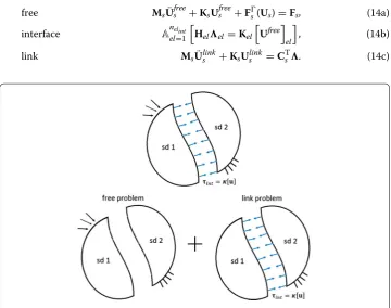
The main idea of the present DD method, common to every non overlapping DD tech-nique (see e.g. [11,40]), is as follows: once the body is divided into parts, the solution is first computed for each single part separately, and then continuity conditions along the interfaces between parts are accounted for to finally obtain the real response of the whole body to the external actions. Each sub-domain is then seen as an independent body, subjected first to external forces and then to interface forces, as shown in Fig.4in the case of two sub-domains only. The time marching procedure is accordingly decomposed into three phases: afreeone, corresponding to the free motion of each unconstrained and unconnected sub-domain subjected to the external loads only; aninterfaceone, in which the interface forces are evaluated; and a link one, in which the above mentioned inter-face forces are applied to contiguous sub-domains to restore continuity [11,13,15,42]. At each time instant, for the sth sub-domain the kinematic fields are so split into two contributions, respectively calledfreeandlink, according to:
Us =Ufrees +Ulinks , (13a)
¨
Us =U¨frees +U¨links . (13b)
This decomposition allows to write thefree,interfaceandlinkproblems [15,41,42] as:
free MsU¨sfree+KsUfrees +Fs(Us)=Fs, (14a)
interface Anelelint=1Helel=KelUfree el
, (14b)
link MsU¨slink+KsUlinks =CTs. (14c)
In Eq. (14):Arepresents the assembling operator; el (el = 1,. . ., nelint) is a vector of Lagrange multipliers for theelth interface element, representing the tractions acting upon the interface itself;Kelis the stiffness matrix of theelth interface element, which reads:
Kel=
el
NTelkNeld, (15)
whereNelis the relevant matrix of nodal shape functions, andkis the local elastic stiffness linking, alongel, tractionsτ to displacement jumps [u] throughτ = k[u].Hel is the interface operator for theelth interface element, that is:
Hel=I+ s∈Simp
βs timp2 Kel
CsM−s1CTs
el, (16)
where:Ms = Ms+βs ts2Ks,βsbeing a coefficient of the Newmark’s time integration algorithm, see [39] as for the notation; tsis either timpor texp, depending on whether an explicit or implicit time integration procedure is adopted for the sth sub-domain; andSimpdenotes the set of uncracked sub-domains, for which the implicit integrator is adopted. In Eq. (16), account has been taken ofβs=0 for the cracking sub-domains (not belonging toSimp); whenever the setSimpchanges because at least one sub-domain starts being cracked and the relevant equation of motion is integrated in time with the explicit integrator,Helhas to be reassembled. Note that the cohesive termFsin Eq. (14)a is clearly nonzero only in the explicit sub-domains.
Let us introduce the time discretization in Eq. (14), focusing on the time interval [tn, tn+1]. Because of the two-time-scales algorithm here exploited (see Fig.3), the free
and link problems have to be solved only once at time tn+1for the linear implicit
sub-domains (integrated with the coarse time scale) and at each intermediate time instanttj withtn≤tj≤tn+1for the explicit non linear sub-domains (integrated with the fine time
scale).
Implicit linear sub-domains
free MsU¨frees,n+1+KsUfrees,n+1=Fs,n+1, (17a)
link MsU¨links,n+1+KsUlinks,n+1=CTsn+1. (17b)
Explicit fractured sub-domains
free MsU¨frees,j +KsUs,jfree+Fs(Us)=Fs,j withj=1, m, (17c)
link MsU¨links,j =CTsj withj=1, m. (17d)
Because of the adopted explicit integration scheme, in Eqs. (17c) and (17d), it holds that Us,j=Ufrees,j =Us,j−1+ texpU˙s,j+ 12 texp2 U¨s,jandUlinks,j =0.
Since the interface problem has to be solved at each time instant of the fine time scale (i.e. the explicit time scale, when crack starts to propagate), thefreedisplacement of the implicit subdomains can be computed at each intermediate time instanttj, according to the linear interpolation proposed in [11], as:
CsUfrees,j =
1− j
m
CsUfrees,n + j mCsU
free
Algorithm 1Domain Decomposition algorithm with elastic interface law (DD)
1: INPUTMs,Ks,t0,tend
2: OUTPUTmechanical solution;Us, ˙Us, ¨Us
3: for(t=t0, tend) do
4: UPDATEt=t+ tref
5: for(s=1, nsd) do
6: UPDATEts=ts+ ts
7: if(ts<t) then
8: SOLVEfree problem
MsU¨frees +KsUsfree+Fs(Us)=Fs
9: end if
10: if(ts=t) then
11: INTERPOLATEfree displacements
CsUfrees,j =
1−mj
CsUs,tfrees− ts+
j mCsU
free s,ts
12: end if
13: end for
14: SOLVEinterface problem
Anelint
el=1
Helel=KelUfreeel 15: for(s=1, nsd) do
16: if(ts=t) then
17: SOLVElink problem
MsU¨links +KsUslink=CTs
18: end if
19: end for
20: end for
The generalized multi-time step explicit–implicit method in the case of multiple sub-domains (s= 1,2,. . ., nsd) is described in Algorithm1. tref stands for the time step of the reference time scale. According to the formulation proposed in [11], such reference time scale is characterized by the smallest time step of the analysis (i.e. the implicit time step in the initial synchronous stage and the explicit time step after crack initiation).
Matching meshes at the interfaces between adjacent sub-domains are considered. This assumption allows to guarantee that the numerical dissipation due to the DD approach, basically linked to the work of the interface forces, does not sensibly affect the energy balance of the system, see [11,13].
The above described DD strategy allows to reduce the computational burden but, in order to remarkably speedup the simulations, a POD-based reduced order modelling scheme is also allowed for. POD, in its snapshot version [43], is initially adopted to reduce the order of the whole problem. Next, as soon as a crack gets incepted in one sub-domain, its numerical model is switched back to the full-order one to properly account for energy dissipation in the process zone and for the changing topology of the crack surfacec; for all the sub-domains within which cracks are not triggered, the solution of the reduced-order equation of motion is still advanced in time with an implicit scheme.
the convergence of the bases towards a steady-state solution can be adopted. The latter approach was shown in [14,15] to provide a further speedup to coupled DD-POD analyses, since convergence can be attained at different time instants in different sub-domains, and so it is not the late sub-model to govern by itself the duration of the training stage.
Since we assume that the whole body behaves elastically up to fracture initiation, the algorithm proposed in [13,29] is used during the training phase to compute the snapshots for each sub-domain. For the problem under study, snapshots do not consist only of the time evolving response of the body to the external loads, but also of the inter-domain continuity. As said, in this phase an implicit, synchronous time stepping procedure is adopted. In [15,42], a thorough discussion of the rationale followed for reduced-order modelling of nonlinear problems was presented; in what follows, only the details relevant to the coupled use of POD and DD, and to the algorithmic handling of the switch from the reduced-order model to the full-order one for the cracked sub-domains are summarized. For thesth sub-domain, the model-specific solution subspace is obtained by monitoring the evolution of the displacement vectorUs. The reduced order form ofUsis written at the sub-domain level as a linear combination of the orthogonal basesαis, is = 1,. . ., rs, according to:
Us= Ns
is=1
αisis =Ass≈ rs
is=1
αisisr =Asrsr, (19)
where: indexris adopted to denote the reduced-order model parameters;Nsis the total number of DOFs in the sub-domain, andrs Nsare the ones retained in the reduced-order model; matrix Asr = [α1s α2s · · · αrs] collects the first rs columns of matrix As =[α1s α2s · · · αNs], each column being a so-called Proper Orthogonal Mode (POM)
of thesth sub-domain; vectorssandsrgather the relevant combination coefficients to provideUs.
To setrsandAsrso as to guarantee the attainment of the minimum discrepancy between
full- and reduced-order representations, during training the snapshotsUjs =Us(tj), j =
1,. . ., nsnapsare collected into the matrixSs∈RNs×nsnaps:
Ss=[U1s U2s · · ·Unsnaps]. (20)
The total number of snapshots for the sth sub-domain,nsnaps, is established a priori; otherwise adaptive procedures controlling the convergence of the bases towards a steady-state solution can be adopted [14,15], updatingrsand the POMs on-the-fly.
The sub-domain matrixSsis thereafter factorized via a SVD procedure, to give:
Ss=LsϒsRsT, (21)
where: Ls ∈ RNs×nsnaps andRs ∈ Rnsnaps×Ns are orthogonal matrices, that respectively gather the so-called left and right singular vectors;ϒs ∈Rnsnaps×Ns is a pseudo-diagonal matrix, whose pivotal entriesυsiiare the singular values of thesth sub-domain response.
rs i=1υs2ii Ns
i=1υs2ii
≥ηs, (22)
thereby retaining in the reduced order model the highest possible oriented energy content. In Eq. (22),ηsis the required energetic accuracy of the reduced order model in thesth sub-domain, established a priori. As a result, the number of POM for each sub-domain,
rs, which does not need to be necessarily the same in all the sub-domains, depends on valuesηs: in the numerical examples presented in this paper,η=0.999 is adopted for all the sub-domains. The described procedure allows to factorize the snapshots matrices of all the sub-domains, and to assemble the reduced bases matrixAsr formed by the firstrs columns of matrixLs.
The singular values and relevant vectors are usually associated to the (oriented) energy content of the system under the given excitation. For structural problems, one may assume that if matrix Ss collects nodal displacements information is obtained concerning the (elastic) energy stored in the bulk of system, whereas if the same matrix collects nodal velocities information is obtained about the system kinetic energy. As the total energy of the system is conserved in the absence of dissipative phenomena (namely, if crack evolution does not take place), the two aforementioned energy terms are related. Anyhow, as pointed out in [46], associating the singular values to the actual elastic and kinetic energies of the system is ”incorrect in principle and may yield misleading results.” So, to ensure the stability and invertibility of the interface operator (16), see also [47], in the snapshot matrix nodal displacements are gathered, and a weak continuity across sub-domains is enforced through the local stiffnessk, see Eq. (15).
Once the reduction matricesAsr have been obtained, the dynamics of each elastic
sub-domain is projected onto the reduced-order space spanned by the relevant POMs in accordance with [15,42]:
Us≈Asrsr, (23a)
˙
Us≈Asr˙sr, (23b)
¨
Us≈Asr¨sr, (23c)
where sr, ˙sr and ¨sr are the reduced-order displacement, velocity and acceleration
vectors. These reduced-order DOFs allow to write the decomposition (14) of the numerical solution for thesth linear elastic sub-domain as:
free Msr¨freesr,n+1=Fsr,n+1−Ksrpsr,n, (24a)
interface Anelelint=1Helel =Kel
Ufree
el
, (24b)
link Msr¨ link
sr,n+1=r,n+1, (24c)
where nowMsr =Msr +βs ts2Ksr, and:
Msr =ATsrMsAsr Ksr =ATsrKsAsr (25a)
Fsr =ATsrFs r =AsTrCTs, (25b)
p
sr,n=s,n+ timp˙s,n+ t 2
imp
1 2−βs
¨
s,n. (26)
p
Note that both the integration scheme and the coarse time step are the same adopted in the training stage while collecting the snapshots. The POD-based reduced order mod-elling is handled in a sub-domain until it remains linear and no topology modifica-tions are involved (i.e. the POD bases are still valid). Once cracking is incepted within a domain, the solution is switched back to the original full-order model for that sub-domain only, because the initial POD bases are not valid any more; propagation inside such sub-domain is handled with the algorithm proposed in [13,29]. Cracking along the interfaces between contiguous sub-domains is instead prevented by the elastic interface model adopted therein. Cohesive elements are inserted on-the-fly, wherever the thresh-oldτmaxis attained. Details regarding the update of the mesh topology can be found in
[13,29,48–50], and are not further discussed here. Because of the adopted explicit integra-tion scheme, the cohesive force vectorFsdepends only on the predictor of the displace-mentspUs,j−1and not on the solution at the end of the current time step and can, thus,
be put at the right hand side of the equation governing thefreeproblem. Consequently, the freeand link problems for the cracked sub-domains at the time instant tj can be formulated as:
MsU¨s,jfree=Fs,j−KspUs,j−1−Fs(pUs,j−1). (27a)
MsU¨s,jlink=CTsj. (27b)
Although the solution for the uncracked sub-domains is computed only at the coarse time scale, the reconstruction of the full orderfreedisplacement along the interfaceUfrees turns out to be necessary, since continuity at the interfaces is imposed at each instanttj of the fine time scale. As the reduced-order free displacement fields for the elastic sub-domains are computed only at the time instants of the implicit scale, they have to be linearly interpolated (see Eq.18) in between starting fromUfree
s = CsAsr free
sr , to finally
evaluate the right hand side of the interface problem Eq. (24b). Algorithm2provides the details of the proposed coupled DD-POD technique.
This procedure is basically the same already proposed in [15], with the only dif-ferent handling of dissipation: while in [15] the activation of plastic deformation was the trigger to switch back from the reduced-order to the full-order model of a sub-domain, here the effective traction τ is tracked along each element face and, as soon as it locally attains the critical threshold corresponding to the material tensile strength τmax, a crack is incepted and so the switch back to the full-order model is activated.
The STEP BACK procedure mentioned at stage 28 of the algorithm is adopted to ensure that the time step is not too large to exceed the mentioned threshold τmax.
Whenever a domain is first traversed by a crack, the switch from the implicit to the explicit time integration procedure is activated too for that sub-domain; it might then happen that timp does not allow to achieve the required resolution along the time axis. Although this entails additional computational costs, to ensure accuracy of the solution or, at least, to avoid exceeding the material strength with the risk of subse-quent artifacts in crack evolution, the solution corresponding to the last time step is re-run by continuously reducing (typically halving, even if adaptive procedure can be also adopted) the time step size, till whenτmaxis not exceeded everywhere in the
Algorithm 2DD-POD
1: INPUTMs,Ks,t0,tend
2: OUTPUTmechanical solution;Us, ˙Us, ¨Us
3: for(t=t0, tend) do
4: UPDATEt=t+ tref
5: for(s=1, nsd) do
6: UPDATEts=ts+ ts
7: if(ts<t) then
8: SOLVEfree problem
elastic sub-domain cracked sub-domain
Msr¨freesr =Fsr−Ksrpsr,0 MsU¨frees =Fs−Ks(pUs,0)−Fs(pUs,0)
9: end if
10: if(ts=t) then
11: INTERPOLATEfree displacements
Ufrees,j =1−mjUs,tfree s− ts+
j mU
free s,ts
12: end if
13: end for
14: SOLVEinterface problem
Anelint
el=1
Helel=KelUfree el
15: for(s=1, nsd) do
16: if(ts=t) then
17: SOLVElink problem
elastic sub-domain cracked sub-domain
Msr¨
link
sr =r MsU¨
link s =CTs
18: end if
19: end for
20: for(s=1, nsd) do
21: COMPUTEthe kinematic fields:
elastic sub-domain cracked sub-domain
U=Asr
free
sr +Asrlinksr U=U
free+Ulink
˙
U=Asr˙frees r +Asr˙
link
sr U˙ =U˙
free+U˙link
¨
U=Asr¨
free sr +Asr¨
link
sr U¨ =U¨
free+U¨link
22: COMPUTEthe stress state in each Gauss point
23: if(crack initiation in thes−th sub-domain) then 24: if(s−th sub-domainis already cracked) then
25: UPDATEthe sub-domain data structure
26: end if
27: if(s−th sub-domainis NOT already cracked) then
28: STEP BACK
29: end if
30: end if
31: end for
32: end for
Numerical examples
The second example concerns the mixed-mode crack propagation, with a crack-path which deviates during the fracture process.
The approach described has been implemented in Fortran 90, and the simulations have been run on a PC featuring an Intel CoreTM i7-2600 CPU @3.4 GHz with a 64 bit operating system. The provided computational gain has been computed asTr−To−Tf−o
f−o ,
whereTr−oandTf−oare the run times (CPU times) corresponding to the full-order (DD only) and reduced-order analyses, respectively.Tr−ogathers both the CPU time required for the training of the ROMs, and the CPU time to advance in time the solution for all the sub-domains. While the training of the ROMs can be optimized through a so-called thin SVD procedure [15,51] in place of the standard one in Eq. (21), the duration of the reduced-order analysis is obviously affected bytend (see Algorithm1). Results collected next thus have to be considered representative, to also show how the selected number of sub-domains can affect the gain.
As mentioned before, the solution for each elastic sub-domain is advanced in time with the Newmark average acceleration scheme featuring γs = 1/2 and βs = 1/4, γs and βsbeing coefficients of the Newmark’s time integration algorithm; while the equations related to the cracked ones are integrated in time with the central difference scheme featuringγs=1/2 andβs=0. In the reduced order simulations, we have always adopted ηs=0.999 for each sub-domain to ensure high accuracy of the solutions.
Double cantilever beam
In this section, a dynamic DCB test [52,53] is considered. The specimen geometry is shown in Fig.5, and the material properties are those proposed in [25], see Table1. The beam lengthLis taken equal to 12 mm, so that the crack propagation is not influenced by the wave reflections from the right end of the beam. The beam has a rectangular cross section of widthBequal to 0.1 mm and height 2 h equal to 0.2 mm. The initial crack length
ais taken equal to 0.4 mm.
The experimental test is performed by slowly opening the beam by means of a wedge and then registering the dynamic crack propagation. The initial conditions are here repro-duced, performing a static elastic analysis under an imposed crack tip opening displace-ment V0. The crack tip is then released and a dynamic analysis is run. Two different
testing conditions, in the following referred to as A and B, have been simulated
consid-Fig. 5 Double cantilever beam test: geometry
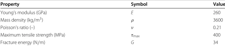
Table 1 Mechanical properties of alumina adopted in the simulations
Property Symbol Value
Young’s modulus (GPa) E 260
Mass density (kg/m3) ρ 3600
Poisson’s ratio (–) ν 0.21
Maximum tensile strength (MPa) τmax 400
ering V0 = 4µm andV0 = 14µm respectively. According to the analytical solutions
proposed, for instance, in [52,53], in the first case the crack stops propagating after reach-ing a plateau value, whereas an unstable fracture propagation is expected in the second case.
The adopted unstructured finite element mesh, featuring quadratic 10-node tetrahedral elements, is characterized by an element size equal to 25µm around the beam axis; this size allows an accurate enough resolution of the stress field within the cohesive zone, whose length is = 55 µm. Conversely, a coarser discretization is adopted near the upper and the bottom sides of the beam and in the elastic part on the right side of the beam, where no crack propagation is expected. The resulting finite element mesh, characterized by 57,896 quadratic tetrahedral elements and 86,936 nodes, is shown in Fig. 6a. Figure6b shows the adopted sub-divisions into subdomains: three different partitions with an increasing number of sub-domains, namely 2,3 and 4, have been considered: one of the sub-domains contains all the elements of coarse size on the right side of the beam (Table2).
In the DD-POD algorithm, the duration of the training phase is set equal to 1.5×10⁻² s and at least 400 snapshots are collected for each sub-domain. Once the training phase ends, the original high order problem in the cracked sub-domain is thus projected onto the reduced space spanned by only 150 POMs in all the sub-division cases.
Figure7shows the crack tip position history for case A. Two different stages can be identified: in the first one, roughly until 0.2 ms, the crack propagation is governed by the stress wave propagation, while in the second one it is determined by a beam-like
Fig. 6 Double cantilever beam test:aspace discretization, andbdomain decomposition into sub-domains Table 2 Double cantilever beam test: number of degrees of freedom and elements corresponding to each sub-domain, for the adopted domain decompositions (see Fig.6b)
Partition Degrees of freedom Elements
DD(2sd) 237,924 23,559 53,713 4183
DD(2sd)-POD 237,924 23,559 53,713 4183
DD(3sd)-POD 112,338 127,059 23,559 25,065 28,648 4183
behavior. Finally, the crack arrests at about 0.7 ms. The crack is always confined in the first sub-domain for all the partitions, except for the 4 sub-domains case, in which also the neighbour sub-domain is reached by the fracture propagation.
To check the performance of the proposed DD-POD algorithm, the numerical results obtained with it are compared with the curve obtained with a domain decomposition simulation performed with a 2 sub-domains partition. In addition, the comparison with the reference analytical solution developed in [53], where the Bernoulli–Euler beam the-ory is employed to model the upper and the lower arm as beams of evolving length, is shown. A noteworthy good agreement of the results can be observed for all the listed simulations even if some discrepancies can be detected between the analytical solution and the numerical ones in the first part of the curve, due to the fact that the approximated analytical solution is not able to describe the effect of the elastic waves on crack propa-gation. Independently of the adopted DD, see also [13], the final lengths at crack arrest differ from the analytical solution by no more than 13%.
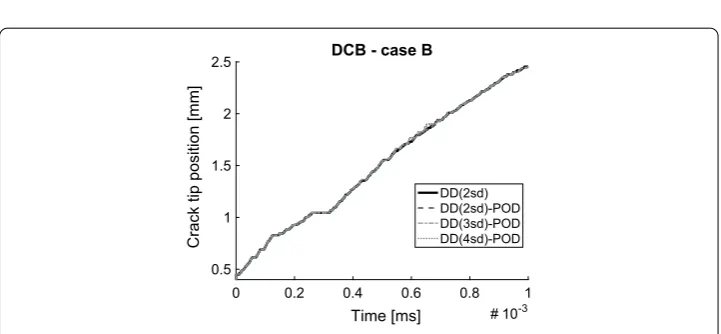
In Fig.8, the outcomes of the numerical simulations performed both with a DD algorithm and with the DD-POD one are compared for case B. The crack remains in the first domain in the case of the 2-subdomains partition, while it crosses more than one
sub-0 0.2 0.4 0.6 0.8 1
Time [ms] #10-3 0.5
1 1.5 2
Crack tip position [mm]
DCB - case A
Analytical solution DD(2sd) DD(2sd)-POD DD(3sd)-POD DD(4sd)-POD
Fig. 7 Double cantilever beam test—case Atime evolution of the crack tip position. Comparison among the reference analytical solution, and the outcomes of the DD approach and of the proposed methodology
0 0.2 0.4 0.6 0.8 1
Time [ms] #10-3 0.5
1 1.5 2 2.5
Crack tip position [mm]
DCB - case B
DD(2sd) DD(2sd)-POD DD(3sd)-POD DD(4sd)-POD
domain, when the partitions into 3 and 4 sub-domains are adopted. All the numerical curves are in good agreement with the reference solution, even if a small perturbation can be observed whenever the crack reaches an interface between two sub-domains.
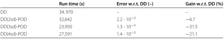
Tables3and4report the results of the total run time for each simulation performed for case A and B respectively. The different sub-divisions of the domain lead to very different computational gains, evaluated with respect to the DD algorithm proposed in [13,29]. As expected, the gain in the case of the 2 sub-domains partition with the DD-POD algorithm is almost negligible, because of the small size of the uncracked subdomain, which collects the coarse size elements at the right side of the body. It could be noticed that the maximum gain is achieved whenever the fracture crosses the minimum number of subdomains, ideally only one subdomain. In such case, a computational gain up to 31% with respect to the DD algorithm proposed in [13,29] is obtained.
Tables3and4also report the error with respect to the reference DD solution, given by theL2norm of the relative discrepancy between the time evolutions of beam deflection
computed with and without the use of POD. All the listed simulations provide an error amounting to less than 3×10⁻³.
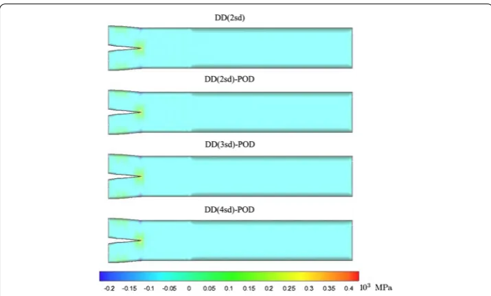
Figures9and10show the contour plots of theσxcomponent (xbeing the direction the beam axis) of the stress vector on the deformed configuration obtained with the reference DD numerical procedure and with the DD-POD algorithm, for case A and B respectively; the good agreement featured by the outcomes of all the simulations, testifies the accuracy of the kinematic fields modelled by the ROMs. Notice that the displacements are amplified to better display the deformed configuration.
Edge-cracked plate under impulsive loading
This section deals with the numerical simulation of the dynamic crack propagation experi-ments performed by [54]. In this test, mixed-mode dynamic loading conditions are created by means of the technique of loading cracks by edge impact, developed by the authors themselves: a specimen with two parallel edge notches is impacted by a projectile moving at a given speedV0 in the direction parallel to the notch; the diameter of the
projec-tile is equal to the distance between the two notches. This configuration determines a
Table 3 Double cantilever beam test—case A: run time, overall error and computational gain with respect to the DD approach
Run time (s) Error w.r.t. DD (–) Gain w.r.t. DD (%)
DD 34,970 – –
DD(2sd)-POD 32,642 2.2·10−3 −6.7
DD(3sd)-POD 23,950 1.3·10−3 −31.5
DD(4sd)-POD 27,591 1.4·10−3 −21.1
All the time data are in seconds (ttot=0.5s)
Table 4 Double cantilever beam test—case B: run time, overall error and computational gain with respect to the DD approach
Run time (s) Error w.r.t. DD (–) Gain w.r.t. DD (%)
DD 35,442 – –
DD(2sd)-POD 33,386 1.8·10−3 −5.8
DD(3sd)-POD 27,822 3.3·10−3 −21.5
DD(4sd)-POD 28,602 4.5·10−3 −19.3
Fig. 9 Double cantilever beam test—case Amap ofσxstress (x being the direction of the beam axis) at the final time instantt=10−3s, on the deformed configuration (displacements amplified 50 times). Comparison among the outcomes of the DD approach and of the proposed methodology
Fig. 10 Double cantilever beam test—case Bmap ofσxstress (x being the direction of the beam axis) at the final time instantt=10−3s, on the deformed configuration (displacements amplified 30 times). Comparison
among the outcomes of the DD approach and of the proposed methodology
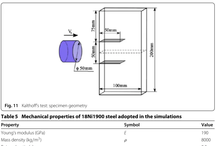
compressive wave that propagates in the middle of the specimen, causing a mixed-mode loading condition at the crack tip. The specimen, schematically represented in Fig.11, is a maraging steel plate 18Ni1900, whose material properties are listed in Table5.
In this case a speedV0 = 16.5 ms is considered; at this low impact velocities, brittle
Fig. 11 Kalthoff’s test: specimen geometry
Table 5 Mechanical properties of 18Ni1900 steel adopted in the simulations
Property Symbol Value
Young’s modulus (GPa) E 190
Mass density (kg/m3) ρ 8000
Poisson’s ratio (–) ν 0.3
Maximum tensile strength (MPa) τmax 800
Fracture energy (N/m) G 22,170
crack propagation is governed by the formation of shear bands ahead of the notch at a negative angle of about 10◦.
The numerical simulation of Kalthoff’s experiment has been discussed in several works in the finite element literature. In [31] the problem of brittle failure was handled by
applying the extended finite element technique (XFEM) on a 2-D finite element model, both with loss of hyperbolicity criterion and tensile stress criterion: the authors reported a crack propagation angle almost equal to 58◦in the former case and to 65◦in the latter one. These results have been compared by the authors with those deriving from simulations performed with inter-element technique, modelled with the Xu–Needleman’s cohesive law [24], in which the fracture propagated with an average angle of almost 55◦. The XFEM method was adopted also by Combescure and co-workers in [55,56], obtaining a crack propagation angle of 65◦.
Because of the twofold symmetry, only one half of the specimen is modelled. An average elements size of 1 mm, smaller than the cohesive length equal to 6.58 mm, is considered. The resulting finite element mesh, characterized by 66,637 quadratic tetrahedral elements
Table 6 Kalthoff’s test: number of degrees of freedom and elements corresponding to each sub-domain, for the adopted domain decompositions (see Fig.12b)
Degrees of freedom Elements
DD(2sd)a-POD 67,785 243,363 14,151 52,486
DD(2sd)b-POD 121,953 188,808 25,845 40,792
and 102,404 nodes, is shown in Fig.12a. Symmetric boundary conditions are imposed at the lower surface of the domain.
Figure12b shows the considered sub-divisions into two sub-domains. In this example, the domain is partitioned in such a way that the crack propagates only in one sub-domain. Table6gathers the number of degrees of freedom and elements corresponding to such sub-domain decompositions.
The duration of the training phase is set equal to 0.01 ms, within which 400 snapshots are collected for each sub-domain.
Figures13,14and15show the time evolution of the crack pattern on the contour plot ofσx component of the stress vector. A deviation in the crack direction with an angle almost equal to 70◦can be observed; the crack does not propagate along a single straight line, because it is constrained to follow the finite element mesh. The results obtained with the two reduced-order simulations are almost indistinguishable from the ones obtained with the DD reference algorithm.
Similarly to the results of the previous example, Table 7shows that the coupled use of DD and POD allows to obtain a computational gain up to 25% with respect to the DD reference solution. Table7shows also that when a partition allows to optimize the
Fig. 15 Kalthoff’s test: map ofσxstress and crack pattern at time instantt=0.06 ms. Comparison among the outcomes of the DD approach and of the proposed methodology
Table 7 Kalthoff’s test: run time, computational gain with respect to the DD approach, and number of POMs retained in the analyses
Run time (s) Gain w.r.t. DD (%) POMs
DD(2sd)a-POD 62,978 −12.3 78
DD(2sd)b-POD 54,364 −24.2 67
All the time data are in seconds (ttot=0.5s)
dimension of the sub-domain which remains elastic (case (2sd)b), the computational gain is higher than in the other case ((2sd)a), even if the total number of the POMs is similar.
Conclusion
In this paper we have proposed a combination of domain decomposition and proper orthogonal decomposition strategies for the efficient simulation of fracture processes in quasi-brittle materials. The obtained results confirm the advantages of the proposed methodology and are extremely encouraging in view of a full exploitation of parallel computing.
model, even after the end of the training stage of the reduced-order models. The results have shown that the computational gain can thus depend much on the partitioning of the whole body into sub-domains. As the propagation path of a main crack, or the pat-tern of cohesive micro-cracking cannot be foreseen under general (mixed-mode) loading conditions, the optimal design of the domain decomposition can be hardly attained.
Work in progress includes the use of strategies similar to the one here proposed for the simulation of irreversible phenomena in the presence of multi-physics coupling.
Authors’ contributions
Authors contributed equally to this work. All authors read and approved the final manuscript.
Acknowledgements
SM gratefully acknowledges the financial support of Fondazione Cariplo through project Safer Helmets, Grant 2013-0716.
Competing interests
The authors declare that they have no competing interests.
Received: 6 February 2016 Accepted: 21 October 2016
References
1. Nadal E, Chinesta F, Díez P, Fuenmayor FJ, Denia FD. Real time parameter identification and solution reconstruc-tion from experimental data using the proper generalized decomposireconstruc-tion. Comput Methods Appl Mech Eng. 2015;296:113–28.
2. Iapichino L, Quarteroni A, Rozza G. Reduced basis method and domain decomposition for elliptic problems in networks and complex parametrized geometries. Comput Math Appl. 2016;71:408–30.
3. Radermacher A, Reese S. Model reduction in elastoplasticity: proper orthogonal decomposition combined with adaptive sub-structuring. Comput Mech. 2014;54(3):677–87.
4. Hinojosa J, Allix O, Guidault P-A, Cresta P. Domain decomposition methods with nonlinear localization for the buckling and post-buckling analyses of large structures. Adv Eng Softw. 2014;70:13–24.
5. Wang KG, Lea P, Farhat C. A computational framework for the simulation of high-speed multi-material fluid-structure interaction problems with dynamic fracture. Int J Numer Methods Eng. 2015;10:585–623.
6. Kerschen G, Golinval JC, Vakakis AF, Bergman LA. The method of proper orthogonal decomposition for dynamical characterization and order reduction of mechanical systems: an overview. Nonlinear Dyn. 2005;41:147–69. 7. Chamoin L, Ladevèze P. Robust control of PGD-based numerical simulations. Eur J Comput Mech. 2012;21:195–207. 8. Cremonesi M, Néron D, Guidault P-A, Ladevèze P. A PGD-based homogenization technique for the resolution of
nonlinear multiscale problems. Comput Methods Appl Mech Eng. 2013;267:275–92.
9. Giner E, Bognet B, Ródenas JJ, Leygueb A, Fuenmayor FJ, Chinesta F. The proper generalized decomposition (PGD) as a numerical procedure to solve 3D cracked plates in linear elastic fracture mechanics. Int J Solids Struct. 2013;50:1710– 20.
10. Niroomandi S, Alfaro I, González D, Cueto E, Chinesta F. Document model order reduction in hyperelasticity: a proper generalized decomposition approach. Int J Numer Methods Eng. 2013;96:129–49.
11. Gravouil A, Combescure A. Multi time step explicit-implicit method for nonlinear structural dynamics. Int J Numer Methods Eng. 2001;50:199–225.
12. Confalonieri F, Corigliano A, Dossi M, Gornati M. A domain decomposition technique applied to the solution of the coupled electro-mechanical problem. Int J Numer Methods Eng. 2013;93:137–59.
13. Confalonieri F, Ghisi A, Cocchetti G, Corigliano A. A domain decomposition approach for the simulation of fracture phenomena in polycrystalline microsystems. Comput Methods Appl Mech Eng. 2014;277:180–218.
14. Corigliano A, Dossi M, Mariani S. Domain decomposition and model order reduction methods applied to the simula-tion of multiphysics problems in MEMS. Comput Struct. 2013;122:113–27.
15. Corigliano A, Dossi M, Mariani S. Model order reduction and domain decomposition strategies for the solution of the dynamic elastic-plastic structural problem. Comput Methods Appl Mech Eng. 2015;290:127–55.
16. Mariani S, Perego U. Extended finite element method for quasi-brittle fracture. Int J Numer Methods Eng. 2003;58:103– 26.
17. Barenblatt G. The mathematical theory of equilibrium cracks in brittle fracture. Adv Appl Mech. 1962;7:55–129. 18. Dugdale D. Yielding of steel sheets containing slits. J Mech Phys Solids. 1960;8:100–4.
19. Hillerborg A, Modeer M, Petersson PE. Analysis of crack formation and crack growth in concrete by means of fracture mechanics and finite elements. Cem Concr Res. 1976;6:773–81.
20. Corigliano A. Formulation, identification and use of interface models in the numerical analysis of composite delami-nation. Int J Solids Struct. 1993;30:2779–881.
21. Zienkiewicz OC, Taylor RL. The finite element method: the basis. 5th ed. Oxford: Butterworth-Heinemann; 2000. 22. Mariani S, Martini R, Ghisi A. A finite element flux-corrected transport method for wave propagation in heterogeneous
solids. Algorithms. 2009;2:1–18.
24. Xu X-P, Needleman A. Numerical simulations of fast crack growth in brittle solids. J Mech Phys Solids. 1994;42:1397– 434.
25. Camacho GT, Ortiz M. Computational modelling of impact damage in brittle materials. Int J Solids Struct. 1996;33:2899–938.
26. Ortiz M, Pandolfi A. Finite-deformation irreversible cohesive elements for three-dimensional crack propagation analy-sis. Int J Numer Methods Eng. 1999;1282:1267–82.
27. Pandolfi A, Guduru PR, Ortiz M, Rosakis AJ. Three dimensional cohesive-element analysis and experiments of dynamic fracture in C300 steel. Int J Solids Struct. 2000;37:3733–60.
28. Zhang ZJ, Paulino GH. Cohesive zone modeling of dynamic failure in homogeneous and functionally graded materials. Int J Plast. 2005;21:1195–254.
29. Confalonieri F. A domain decomposition approach for the simulation of fracture phenomena in polycrystalline microsystems. Ph.D. thesis, Politecnico di Milano, 2013.
30. Bolzon G, Corigliano A. Finite elements with embedded displacement discontinuity: a generalized variable formula-tion. Int J Numer Methods Eng. 2000;49:1227–66.
31. Belytschko T, Chen H, Xu J, Zi G. Dynamic crack propagation based on loss of hyperbolicity and a new discontinuous enrichment. Int J Numer Methods Eng. 2003;58:1873–905.
32. Moes N, Belytschko T. Extended finite element method for cohesive crack growth. Eng Fract Mech. 2002;69:813–33. 33. Corigliano A, Cacchione F, Frangi A, Zerbini S. Numerical modelling of impact rupture in polysilicon microsystems.
Comput Mech. 2007;42:251–9.
34. Mariani S, Ghisi A, Corigliano A, Zerbini S. Multi-scale analysis of MEMS sensors subject to drop impacts. Sensors. 2007;7:1817–33.
35. Mariani S, Martini R, Ghisi A, Corigliano A, Simoni B. Monte carlo simulation of micro-cracking in polysilicon mems exposed to shocks. Int J Fract. 2011;167:83–101.
36. Irwin GR. Structural aspects of brittle fracture. Appl Mater Res. 1964;3:65–81.
37. Espinosa HD, Zavattieri PD. A grain level model for the study of failure initiation and evolution in polycrystalline brittle materials. Part I: theory and numerical implementation. Mech Mater. 2003;35:333–64.
38. Espinosa HD, Zavattieri PD. A grain level model for the study of failure initiation and evolution in polycrystalline brittle materials. Part II: Numerical examples. Mech Mater. 2003;35:365–94.
39. Hughes TJR. The finite element method: linear static and dynamic finite element analysis. Mineola: Dover Publications; 2000.
40. Mahjoubi N, Gravouil A, Combescure A. Coupling subdomains with heterogeneous time integrators and incompatible time steps. Comput Mech. 2009;44:825–43.
41. Corigliano A, Dossi M, Mariani S. Recent advances in computational methods for microsystems. Adv Mater Res. 2013;745:13–25.
42. Dossi M. Combined model order reduction and domain decomposition strategies for the solution of non-linear and multi-physics structural problems. Ph.D. thesis, Politecnico di Milano, 2015.
43. Sirovich L. Turbulence and the dynamics of coherent structures. I-coherent structures. II-symmetries and transforma-tions. III-dynamics and scaling. Q Appl Math. 1987;45:561–90.
44. Azam SE, Mariani S. Investigation of computational and accuracy issues in POD-based reduced order modeling of dynamic structural systems. Eng Struct. 2013;54:150–67.
45. Feeny BF, Kappagantu R. On the physical interpretation of proper orthogonal modes in vibrations. J Sound Vib. 1998;211:607–16.
46. Chatterjee A. An introduction to the proper orthogonal decomposition. Curr Sci. 2000;78:808–17.
47. Faucher V, Combescure A. Local modal reduction in explicit dynamics with domain decomposition. Part 2: specific interface treatment when modal subdomains are involved. Int J Numer Methods Eng. 2004;61:69–95.
48. Pandolfi A, Ortiz M. Solid modeling aspects of three-dimensional fragmentation. Eng Comput. 1998;14:287–308. 49. Pandolfi A, Ortiz M. An efficient adaptive procedure for three-dimensional fragmentation simulations. Eng Comput.
2001;18:148–59.
50. Paulino GH, Celes W, Espinha R, Zhang ZJ. A general topology-based framework for adaptive insertion of cohesive elements in finite element meshes. Eng Comput. 2007;24:59–78.
51. Zhang Y, Combescure A, Gravouil A. Efficient hyper reduced-order model (hrom) for parametric studies of the 3d thermo-elasto-plastic calculation. Finite Elem Anal Des. 2015;102–103:37–51.
52. Kanninen M. A dynamic analysis of unstable crack propagation and arrest in the DCB test specimen. Int J Fract. 1974;10:415–30.
53. Freund L. Dynamic fracture mechanics. Cambridge: Cambridge university press; 1990. 54. Kalthoff JF. Modes of dynamic shear failure in solids. Int J Fract. 2000;101:1–31.
55. Réthoré J, Gravouil A, Combescure A. An energy-conserving scheme for dynamic crack growth using the extended finite element method. Int J Numer Methods Eng. 2005;63:631–59.