Component-based reduced basis for parametrized symmetric eigenproblems

R E S E A R C H A R T I C L E

Open Access

Component-based reduced basis for

parametrized symmetric eigenproblems

Sylvain Vallaghé

, Phuong Huynh

, David J Knezevic

, Loi Nguyen

and Anthony T Patera

*Correspondence: [email protected] 1Massachusetts Institute of Technology, 77 Mass Ave, 02139 Cambridge MA, USA

4Swiss Federal Institute of Technology in Lausanne, Station 8, 1015 Lausanne, Switzerland Full list of author information is available at the end of the article

Abstract

Background: A component-based approach is introduced for fast and flexible solution of parameter-dependent symmetric eigenproblems.

Methods: Considering a generalized eigenproblem with symmetric stiffness and mass operators, we start by introducing a “σ-shifted” eigenproblem where the left hand side operator corresponds to an equilibrium between the stiffness operator and a weighted mass operator, with weight-parameterσ >0. Assuming thatσ =λn>0, thenthreal positive eigenvalue of the original eigenproblem, then the shifted eigenproblem reduces to the solution of a homogeneous linear problem. In this context, we can apply the static condensation reduced basis element (SCRBE) method, a domain synthesis approach with reduced basis (RB) approximation at the intradomain level to populate a Schur complement at the interdomain level. In the Offline stage, for a library of archetype subdomains we train RB spaces for a family of linear problems; these linear problems correspond to various equilibriums between the stiffness operator and the weighted mass operator. In the Online stage we assemble instantiated subdomains and perform static condensation to obtain the “σ-shifted” eigenproblem for the full system. We then perform a direct search to find the values ofσthat yield singular systems, corresponding to the eigenvalues of the original eigenproblem.

Results: We provide eigenvaluea posteriorierror estimators and we present various numerical results to demonstrate the accuracy, flexibility and computational efficiency of our approach.

Conclusions: We are able to obtain large speed and memory improvements

compared to a classical Finite Element Method (FEM), making our method very suitable for large models commonly considered in an engineering context.

Keywords: Eigenproblems; Domain synthesis; Reduced basis;A Posteriorierror estimation

Background

In structural analysis, eigenvalue computation is necessary to find the periods at which a structure will naturally resonate. This is especially important for instance in building engi-neering, to make sure that a building’s natural frequency does not match the frequency of expected earthquakes. In the case of resonance, a building can endure large deforma-tions and important structural damage, and possibly collapse. The same consideradeforma-tions apply to automobile and truck frames, where it is important to avoid resonance with the engine frequencies. Eigenproblems also appear when considering wind loads, rotating

machinery, aerospace structures; in some cases it is also desirable to design a structure for resonance, like certain microelectromechanical systems.

With improvement in computer architecture and algorithmic methods, it is now pos-sible to tackle large-scale eigenvalue problems with millions of degrees of freedom; however the computations are still heavy enough to preclude usage in a many-query context, such as interactive design of a parameter-dependent system. In this paper, we present an approach for fast solution of eigenproblems on large systems that present a component-based structure – such as building structures.

For the numerical solutions of partial differential equations (PDE) in component-based systems, several computational methods have been introduced to take advantage of the component-based structure. The main idea of these methods is to perform domain decomposition, and to use a common model order reduction for each family of similar components. The first and classical approach is the component mode synthesis (CMS) as introduced in [1,2]: it uses the eigenmodes of local constrained eigenvalue problems for the approximation within the interior of the component and static condensation to arrive at a (Schur complement) system associated with the coupling modes on the inter-faces or ports. One drawback of the CMS approach is the rather slow convergence of eigenmodal expansions. In contrast the reduced basis element (RBE) method [3] employs a reduced basis expansion [4] within each component or subdomain and Lagrange mul-tipliers to couple the local bases and hence compute a global solution of the considered parameter dependent partial differential equation for each admissible parameter. The RBE method thus profits from the fact that RB approximations yield a rapid and in many cases exponential convergence [5].

A combination of RB methods and domain decomposition approaches has for instance also been considered in [6,7]. Similarly RB methods have been employed in the frame-work of a multi-scale finite element method to construct local reduced spaces for the approximation of fine-scale features on the coarse grid elements in [8,9], where the latter corresponds to the “components” in the RBE method.

In [10], a static condensation RBE (SCRBE) approach is developed for elliptic problems. It brings together ideas of CMS and RBE by considering standard static condensation at the interdomain level and then RB approximation at the intradomain level. In an Offline stage performed once, the RB space for a particular component is designed to reflect all possible function variations on the component interfaces (which we shall denote “ports”); components are thus completely interchangeable and interoperable. During the Online stage, any system can be assembled from multiple instantiations of components from a predefined library; we can then compute the system solution for different values of the component parameters in a prescribed parameter domain. The Online stage of the SCRBE is much more flexible than both the Online stage for the standard RB method, in which the system is already assembled and only parametric variations are permitted, and the Online stage of the classical (non-static-condensation) RBE method, in which the RB intradomain spaces already reflect anticipated connectivity.

of the shiftσthat correspond to singular systems. Second, we providea posteriorierror estimators of the eigenvalues, not only with respect to RB approximations but also in the context of port reduction.

In the context of CMS approaches for eigenproblems, out method provides some important features: treatment of parameter-dependent systems (as explained above), optimal convergence, and port reduction. The classical CMS only achieves a polynomial convergence rate [11,12] with respect to the number of eigenmodes used at the intrado-main level. This can be improved to an infinite convergence rate by using overlapping components [12], but at the expense of losing simplicity and flexibility of component connections. Our method somehow provides an optimal trade-off since it retains the interface treatment of classical CMS – allowing flexibility of component connections – while achieving an exponential convergence rate with respect to the size of RB spaces at the intradomain level.

We also provide port reduction so as to increase even more the speed up. Recent CMS contributions consider several port economizations (or interface reduction strategies): an eigenmode expansion (with subsequent truncation) for the port degrees of freedom is proposed in [11,13]; an adaptive port reduction procedure based on a posteriori error estimators for the port reduction is proposed in [14]; and an alternative port reduction approach, with a different bubble function approximation space, is proposed for time-dependent problems in [15]. We can not directly apply CMS port reduction concepts in the parameter-dependent context, as the chosen port modes must be able to provide a good representation of the solution for any value of the parameters. In this paper, we adapt to parameter-dependent eigenproblems a port approximation and a posteriori error bound framework introduced in [16] for parameter-dependent linear elliptic problems.

The paper proceeds as follows. In Section ‘Formulation’, we present the general eigen-problem and its shifted formulation; we then describe the static condensation procedure. In Section ‘Reduced basis static condensation system’, we add reduced basis approxi-mations and developa posteriori error estimators for the eigenvalues with respect to the corresponding values obtained by the “truth” static condensation of Section ‘Formu-lation’. In section ‘Port reduction’, we introduce port reduction and provide as wella posteriorierror estimators for the eigenvalues. In Section ‘Computational aspects’, we give an overview of the computational aspects of the method. This section somehow brings together all of the previous sections in a compact presentation, and we suggest the reader to often go back to Section ‘Computational aspects’ in order to get a higher level description of the method. Finally, in Section ‘Results and discussion’, we present numer-ical results to illustrate the computational efficiency of the approach. We first consider simple bridge structures for which we examine the error estimates. We finish with an industrial scale example to show the method’s potential to tackle large systems.

Methods Formulation Problem statement

We suppose that we are given an open domain⊂Rd,d=1, 2 or 3, with boundary∂. We then letXdenote the Hilbert space

X≡v∈H1():v|∂D =0

where∂D ⊂ ∂is the portion of the boundary on which we enforce homogeneous Dirichlet boundary conditions. We suppose that X is endowed with an inner product (·,·)Xand induced norm · X. Recall that for any domainOinRd,

H1(O)≡v∈L2(O):∇v∈(L2(O))d,

whereL2(O)≡

vmeasurable overO:

Ov 2_finite

.

Furthermore, letY ≡L2().

We now introduce an abstract formulation for our eigenvalue problem. For anyμ∈D, let a(·,·;μ) : X×X → R, andm(·,·;μ) : X×X → Rdenote continuous, coercive, symmetric bilinear form with respect toXandY, respectively. We suppose thatXN ⊂X is a finite element space of dimensionN. Given a parameterμ ∈ D ⊂ RP, whereDis our parameter domain of dimensionP, we find the set of eigenvalues and eigenvectors (λ(μ),u(μ)), whereλ(μ)∈R>0andu(μ)∈XNsatisfy

a(u(μ),v;μ) = λ(μ)m(u(μ),v;μ), ∀v∈XN, (1)

m(u(μ),u(μ);μ) = 1. (2)

We assume that the eigenvaluesλn(μ)are sorted such that 0< λ1(μ) ≤ λ2(μ) . . . ≤

λN(μ), and to each eigenvalueλn(μ)we associate a corresponding eigenvectorun(μ). We can have multiplicities greater than one and hence we can have equal succes-sive eigenvaluesλn(μ) = · · · = λn+k(μ) but each associated to linearly independent eigenvectors.

The parametric dependence of the problem usually takes the form of variable PDE coef-ficients or variable geometry. For instance, in linear elasticity, the vectorμcan contain the different Young’s modulus values of different subdomains, as well as the parameters of some mapping function describing the geometrical variability.

We now define a surrogate eigenvalue problem that will be convenient for subsequent developments. For a given “shift factor”σ ∈ R≥0, we modify (1), (2) such that for any

μ∈D, we findτ(μ,σ)∈Randχ(μ,σ)∈XN that satisfy

B(χ(μ,σ),v;μ;σ) = τ(μ,σ)a(χ(μ,σ),v;μ), ∀v∈XN, (3)

a(χ(μ,σ),χ(μ,σ);μ)= 1. (4)

Here

B(w,v;μ;σ)≡a(w,v;μ)−σm(w,v;μ) (5)

is our “shifted” bilinear form. Note that we change the bilinear form on the right hand side fromm(·,·)toa(·,·), which corresponds to a different norm. This choice is motivated by error estimation, presented later in the paper, as it permits to derive relative error estimates for the eigenvalueλn(μ).

We also sort the set of eigenvalues such thatτ1(μ,σ)≤τ2(μ,σ) . . .≤τN(μ,σ)– note that due to the shift the first eigenvalues can now be negative. It is clear thatχn(μ,σ) =

1

√

λn(μ)un(μ)for anyσ ∈R, so we shall henceforth writeχn(μ). Also

τn(μ,σ)= λn_λ(μ)−σ n(μ)

so that

τn(μ,σ) >0, if 0≤σ < λn(μ), (7)

τn(μ,σ)=0, if σ =λn(μ), (8)

τn(μ,σ) <0, if σ > λn(μ), (9)

forn=1,. . .,N.

Remark 2.1. The reason for introducing the surrogate eigenvalue problem (3) is that when the condition (8) is achieved, the right hand side of (3) vanishes and we can consider the left hand side in isolation as a linear problem to which we apply the SCRBE method, as described in the following sections. Two points have to be make clear about the parameter σ:

• σ is meant to approximate a given eigenvalueλn(μ)of the original eigenproblem (1) by virtue of property (8),

• the value for whichσ =λn(μ)will be automatically determined by a direct search algorithm as presented in Section ‘Eigenvalue computation’.

Static condensation

We now move to the component level. We suppose that the system domain is natu-rally decomposable intoIinterconnected parametrized components. Each componenti is associated with a subdomaini, where

=

I

i=1

i, i∩i = ∅, fori=i.

We now introduce the notion of “port” that is commonly used in the literature related to CMS methods. A port corresponds to the interface shared by two components that are connected together. When looking at the global system, we will describe the ports as global, whereas when considering a single component, we will describe the ports as local. We say that componentsiandiare connected at global portpifi∩i = p = ∅, where 1 ≤ p ≤ n andn is the total number of global ports in the system. We also say thatγ_ij= pandγj

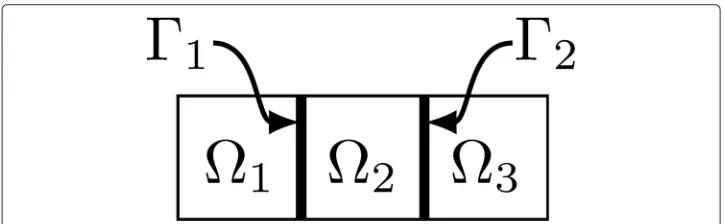
i =pare local ports of componentsiandirespectively, where 1≤j≤nγ_i is the total number of local ports in componenti. Figure 1 shows an example of a three component system, with the corresponding global and local port definitions.

Figure 1 An example of system composed of three components, of indices 1, 2 and 3, corresponding to the subdomains1,2,3. This system has two global ports of indices 1 and 2, corresponding to the interfaces 1=1∩2and2=2∩3. Component 1 has one local portγ1

1 =1, component 2 has two local portsγ1

We assume that the FE spaceXN conforms to our components and ports, hence we can define the discrete spacesX_iN andZ_pNthat are simply the restrictions ofXNto com-ponentiand global portp. For giveni, letX_iN_;0 denote the “component bubble space” — the restriction ofXN toi with homogeneous Dirichlet boundary conditions on each

γj

i, 1≤j≤n

γ

i,

XN_i;0 ≡

v|i:v∈XN; v|_γj

i =0, 1≤j≤n

γ

i

.

We denote byN_pthe dimension of the port spaceZN_p associated with global portp, and we say that the global portphasN_pdegrees of freedom (dof ). For each component i, we denote byk a local port dof number, andKithe total numbers of dof on its local ports, such that 1≤k≤Ki. We then introduce the mapPi(k)=(p,k)which associate a local port dofkin componentito its global port representation: global portpand dof k, 1≤k≤N_p.

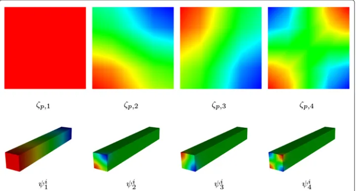
To formulate our static condensation procedure we must first introduce the basis func-tions for the port spaceZN_p as{ζp,1,· · ·,ζp,N

p}. The particular choice for these functions

is not important for now, but it becomes critical when dealing with port reduction – we refer to Section ‘Port reduction’. For a local port dof numberksuch thatPi(k)=(p,k), we then introduce the interface functionψ_ki ∈X_iN, which is the harmonic extension of

the associated port space basis function into the interior of the component domaini, and satisfies

i

∇ψi

k· ∇v=0, ∀v∈XiN;0, (10)

ψi k =

ζp,k onp

0 onγ_ij=p, 1≤j≤nγi.

(11)

We show in Figure 2 an example of port basis functions and interface functions.

If componentsiandjare connected, then for each matching local port dofskiandkj such thatPi(ki)=Pj(kj)=(p,k), we define the global interface functionp,k∈XN as

p,k = ⎧ ⎪ ⎨ ⎪ ⎩ ψi ki oni

ψj kj onj

0 elsewhere.

(12)

We will now develop an expression forχn(μ)which just involves dof on the ports by virtue of elimination of the interior dof given thatσ =λn(μ)– starting from (13) to finally arrive at (18). Let us suppose that we setσ =λn(μ)(for somen) so that the right-hand side of (3) vanishes. Then, forχn(μ)∈XNwe have

B(χn(μ),v;μ;σ)=0, for allv∈XN.

We then expressχn(μ)∈XNin terms of “interface” and “bubble” contributions,

χn(μ)= I

i=1

bi(μ,σ)+ n

p=1 N

p

k=1

Up,k(μ,σ)p,k, (13)

where theUp,k(μ,σ)are interface function coefficients corresponding to the portp, and

bi(μ,σ)∈XiN;0. Hereχnis independent ofσ, but we shall see shortly that we will needbi andU_k,pto beσ-dependent in general.

We then restrict to a single componentito obtain

Bi(χn(μ),v;μ;σ)=0, for allv∈XiN;0, (14)

where Bi(w,v;μ;σ) ≡ ai(w,v;μ)− σmi(w,v;μ), and where ai and mi indicate the restrictions ofaandmtoi, respectively. Substitution of (13) into (14) leads to

Bi(bi(μ,σ),v;μ;σ)+ Ki

k=1

U_Pi(k)(μ,σ)Bi(ψi,k,v;μ;σ)=0, (15) for allv∈X_iN_;0.

It can be shown from linearity of the above equation that we can reconstructbi(μ,σ)as

bi(μ,σ)= Ki

k=1

U_Pi(k)(μ,σ)b_i,k(μ,σ), wherebi,k(μ,σ)∈XiN;0satisfies

Bi(bi,k(μ,σ),v;μ;σ)= −Bi(ψi,k,v;μ;σ), ∀v∈XiN;0. (16)

Let (λi,n(μ),χi,n(μ)) ∈ R× XiN;0 denote an eigenpair associated with the n local

eigenproblem

ai(χi,n(μ),v;μ)=λi,n(μ)mi(χi,n(μ),v;μ), ∀v∈XiN;0, (17)

then, since

inf v∈X_i;0N

Bi(v,v;μ;σ)

v2_X,i = v∈infX_i;0N

ai(v,v;μ)−σmi(v,v;μ)

v2_X,i

≥ inf v∈X_i;0N

ai(v,v;μ)−σmi(v,v;μ)

mi(v,v;μ)

inf v∈XN_i;0

mi(v,v;μ)

v2_X,i

= (λi,1(μ)−σ) inf

v∈X_i;0N

mi(v,v;μ)

the bilinear formBi(·,·;μ;σ)is coercive onX_iN_;0ifσ < λi,1(μ), whereλi,1(μ)is the

small-est eigenvalue of (17). Hence (16) has a unique solution under this condition. Note that we expect thatλi,1(μ) > λ1(μ), and evenλi,1(μ) > λn(μ)forn=2 or 3 or 4 — of course in practice the balance between λn andλi,n will depend on the details of a particular problem.

Now for 1≤k≤N_pand eachp, let p,k(μ,σ)=p,k+

i,ks.t.Pi(k)=(p,k)

b_i,k(μ,σ),

and let us define the “skeleton” spaceXS(μ,σ)as

X_S(μ,σ)≡span{_p,k(μ,σ): 1≤p≤n, 1≤k≤N_p}. This space is of dimensionnsc=n

p=1Np.

Remark 2.2. Note that the interface functions are intermediate quantities that are com-pleted with bubble functions. Although the interface functions are the result of a simple harmonic lifting with the homogeneous Laplace operator, the subsequent bubble functions are computed based on the problem-dependent a and m bilinear forms, hence they capture the possible heterogeneities intrinsic to the problem. Hence the skeleton space X_S(μ,σ)is suitable for approximation.

We restrict (13) to a single componentito see that forσ =λn(μ)we obtain

χn(μ)|i= Ki

k=1

U_Pi(k)(μ,σ)

bi,k(μ,σ)+ψi,k

.

This then implies

χn(μ)= n

p=1 Np

k=1

U_p,k(μ,σ) p,k(μ,σ)∈XS(μ,σ). (18)

Then, forσ = λn(μ)andμ ∈ D, we are able to solve for the coefficientsUp,k(μ,σ) from the static condensation eigenvalue problem onX_S(μ,σ): findχn(μ) ∈ XS(μ,σ), such that

B(χn(μ),v;μ;σ) = 0, ∀v∈XS(μ,σ), (19)

a(χn(μ),χn(μ);μ)= 1. (20)

We now relax the conditionσ = λn(μ) to obtain the following problem: For σ ∈ [ 0,σmax] andμ∈D, find(τn(μ,σ),χn(μ,σ))∈(R,XS(μ,σ)), such that

B(χn(μ,σ),v;μ;σ) = τn(μ,σ)a(χn(μ;σ),v;μ), ∀v∈XS(μ,σ), (21)

a(χ_n(μ,σ),χ_n(μ,σ);μ) = 1. (22)

It is important to note that this new eigenproblem (21) (22) differs from (3) (4) in two ways: first, we consider a subspaceX_S(μ,σ)ofXN, and as a consequenceτn(μ,σ) ≥

τn(μ,σ); second, the subspaceXS(μ,σ), unlikeXN, depends onσ, and furthermore only forσ=λndoes the subspaceXS(μ,σ)reproduce the eigenfunctionχn(μ). We now show

(i) τn(μ,σ)≥τn(μ,σ),n=1,. . .,dim(XS(μ,σ)), (ii) τn(μ,σ)=0if and only ifσ =λn(μ),

(iii) σ =λn(μ)if and only if there exists somensuch thatτn(μ,σ)=0.

Proof.

(i) The casen=1follows from the Rayleigh quotients

τ1(μ,σ)= inf

w∈XN

B(w,w;μ;σ)

a(w,w;μ) , (23)

and

τ1(μ,σ)= inf

w∈X_S(μ,σ)

B(w,w;μ;σ)

a(w,w;μ) , (24)

and fact thatX_S(μ,σ)⊂XN.

Forn>1, the Courant-Fischer-Weyl min-max principle [17] states that for an arbitraryn-dimensional subspace ofXN,Sn, we have

ηn(μ,σ)≡max w∈Sn

B(w,w;μ;σ)

a(w,w;μ) ≥τn(μ,σ). (25)

LetSn≡span{χm(μ,σ),m=1,. . .,n} ⊂XS(μ,σ). Thenηn(μ,σ)=τn(μ,σ), and the result follows.

(ii) This equivalence is due to (8).

(iii) (⇐) Supposeσ =λn(μ)for somen, then by constructionχn(μ,σ)∈XS(μ,σ).

Since the same operatorBappears in both (19) and (21), it follows thatχn(μ,σ)is also eigenmode for (21), (22) with corresponding eigenvalue 0. That is, for somen,

τn(μ,σ)=0is an eigenvalue of (21), (22).

(⇒) Supposeτn(μ,σ)=0for some indexn. Thenχn(μ,σ)satisfies (19), (20), or equivalently, (3), (4) forτn(μ,σ)=0. From part (ii) of this Proposition, this implies thatσ=λn(μ).

Remark 2.3. Regarding our method, the main result is 2.1(iii), which informs on how to recover eigenvalues of the original problem (3), (4) from the shifted and condensed prob-lem (21), (22): we look for the values ofσ such that (21), (22) has a zero eigenvalue. Note that in 2.1(iii), the equivalence betweenτn(μ,σ)=0andσ =λn(μ)possibly happens for

To assemble an algebraic system for the static condensation eigenproblem, we insert (18) into (21), (22) to arrive at

n

p=1 N

p

k=1

Up,k(μ,σ)B(p,k(μ,σ),v;μ;σ)

=τ(μ,σ) n

p=1 N

p

k=1

U_p,k(μ,σ)a(_p,k(μ,σ),v;μ;σ), ∀v∈X_S, (26)

n

p=1 Np

k=1

Up,k(μ,σ)a(p,k(μ,σ),p,k(μ,σ);μ;σ)=1. (27)

We now define our local stiffness and mass matricesAi(μ,σ),Mi(μ,σ) ∈ RKi×Ki _for

componenti, which have entries

Ai_k,k(μ,σ) = ai(ψi,k+bi,k(μ,σ),ψi,k+bi,k(μ,σ);μ),

Mi_k,k(μ,σ) = mi(ψi,k+bi,k(μ,σ),ψi,k+bi,k(μ,σ);μ),

for 1 ≤ k,k ≤ Ki. We may then assemble the global system with matrices B(μ,σ),A(μ,σ)∈Rnsc×nsc_{, of dimensionn}

sc=

_n

p=1Np: given aσ ∈Randμ∈D, we consider the eigenproblem

B(μ,σ)V(μ,σ) = τ(μ,σ)A(μ,σ)V(μ,σ), (28)

V(μ,σ)TA(μ,σ)V(μ,σ) = 1, (29)

where

B(μ,σ)≡A(μ,σ)−σM(μ,σ). (30)

As explained above, in order to find the eigenvalues of the original problem (3), (4), we need to find the values ofσ for which (28), (29) has a zero eigenvalue. When performing this search, for each new value ofσ that is considered, we need to perform the assembly of the static condensation system (28), which involves many finite element computa-tions at the component level in order to get the bubble funccomputa-tions (16), and is potentially costly. Note that we also need to reassemble (28) when the parametersμof the problem change. In order to dramatically reduce the computational cost of this assembly, we will use reduced order modeling techniques as described in the next Sections ‘Reduced basis static condensation system’ and ‘Port reduction’.

Reduced basis static condensation system Reduced basis bubble approximation

In the static condensation reduced basis element (SCRBE) method [10], we replace the FE bubble functionsbi,k(μ,σ)with reduced basis approximations. These RB approximations are significantly less expensive to evaluate (following an RB “offline” preprocessing step) than the original FE quantities, and hence the computational cost associated with the formation of the (now approximate) static condensation system is significantly reduced. We thus introduce the RB bubble function approximations

˜

for a parameter domain(μ,σ)∈D×[ 0,σmax], where

σmax=σmin

μ∈D1min≤i≤Iλi,1(μ). (32) Hereσ(<1)is a “safety factor” which ensures that we honor the conditionσ < λi,1(μ)

for all 1≤i≤I. Next, we let

p,k(μ,σ)=p,k+

i,kis.t.Pi(ki)=(p,k)

˜

bi,ki(μ,σ),

and define our RB static condensation spaceXS(μ,σ)⊂XNas

X_S(μ,σ)=span{p,k(μ,σ): 1≤p≤n, 1≤k≤Np}. (Note thatX_S(μ,σ)⊂X_S(μ,σ)).

Remark 3.1. As opposed to CMS where the static condensation space is built from local component natural modes, the RB static condensation spaceX_S(μ,σ)is built from RB bubbles that can accommodate for any global mode shape thanks to their (μ,σ) parametrization. The only restriction is due to condition (32) which means that we only ensure to capture global modes for which the wavelength is typically greater than a component’s size.

We then define the RB eigenproblem: given(μ,σ)∈ D×[ 0,σmax], find the eigenpairs

(τn(μ,σ),Vn(μ,σ))that satisfy

B(μ,σ)V(μ,σ) =τ(μ,σ)A(μ,σ)V(μ,σ), (33)

V(μ,σ)TA(μ,σ)V(μ,σ) = 1, (34)

whereB(μ,σ),A(μ,σ)are constructed component-by-component from

Ai_k,k(μ,σ) = ai(ψi,k+ ˜bi,k(μ,σ),ψi,k+ ˜bi,k(μ,σ);μ), (35)

Mi_k,k(μ,σ) = mi(ψi,k+ ˜bi,k(μ,σ),ψi,k+ ˜bi,k(μ,σ);μ), (36)

for 1≤k,k≤Ki, and where

_Bi_(μ,σ)≡Ai_{(μ,σ)−σM}i_{(μ,σ). (37)}

Reduced basis error estimator

We now consider error estimation for our RB approximations. In order to derive error estimates, we will use Hypothesis A.1 which is related to Remark 2.3, and reads

σ =λn(μ)⇔τn(μ,σ)=0.

Note that this hypothesis is solely used for error estimation, the computational method itself does not rely on this assumption.

First, sinceXS(μ,σ)⊂XN, by the same argument as part (i) of Proposition 2.1, we have

Corollary 3.1.

We define the residualri,k(·;μ,σ):XiN;0 →Rfor 1≤k≤Ki, and 1≤i≤Ias

ri,k(v;μ,σ)= −Bi(ψi,k+ ˜bi,k(μ,σ),v;μ,σ), ∀v∈XiN;0,

and the error bound [4]

bi,k(μ,σ)− ˜bi,k(μ,σ)X,i≤i,k(μ,σ)= Ri,k(μ ,σ) αLB

i (μ,σ) ,

where

Ri,k(μ,σ)= sup v∈X_i;0N

ri,k(v;μ,σ)

vX,i

is the dual norm of the residual, andαLB_i (μ,σ)is a lower bound for the coercivity constant

αi(μ,σ)= inf w∈X_i;0N

Bi(w,w;μ,σ)

w2_X,i ,

that can be derived by hand for simple cases, or computed using a successive constraint linear optimization method [18].

We now assume that Hypothesis A.1 holds. Suppose we have foundσn, thenth“shift” such thatB(μ,σn)has a zero eigenvalue, i.e. we haveτn(μ,σn)= 0. Then our RB-based approximation to thentheigenvalue isλ˜n(μ)=σn. We will now develop a first order error estimator forτn(μ,σn). We have

B(μ,σn)V(μ,σn)=τn(μ,σn)A(μ,σn)V(μ,σn),

and hence with B(μ,σn) ≡ B(μ,σn) + δB(μ,σn), A(μ,σn) ≡ A(μ,σn) +δA(μ,σn), V(μ,σn)≡V(μ,σn)+δV(μ,σn), we obtain

(B(μ,σn)+δB(μ,σn))(V(μ,σn)+δV(μ,σn))=

τn(μ,σn)(A(μ,σn)+δA(μ,σn))(V(μ,σn)+δV(μ,σn)). (39)

Expansion of the above expression yields

B(μ,σn)δV(μ,σn)+δB(μ,σn)V(μ,σn)+δB(μ,σn)δV(μ,σn)=

τn(μ,σn)(A(μ,σn)V(μ,σn)+A(μ,σn)δV(μ,σn)+

δA(μ,σn)V(μ,σn)+δA(μ,σn)δV(μ,σn)), (40)

where the identityB(μ,σn)V(μ,σn) = 0 has been employed. We then multiply through byV(μ,σn)T and note that

V(μ,σn)TB(μ,σn)δV(μ,σn)=δV(μ,σn)TB(μ,σn)V(μ,σn)=0, V(μ,σn)TA(μ,σn)V(μ,σn)=1

and neglect higher order terms to obtain

τn(μ,σn)≈V(μ,σn)TδB(μ,σn)V(μ,σn). (41)

We then have the following bound

|V(μ,σn)TδB(μ,σn)V(μ,σn)|

≤

I

i=1

Ki

k=1

I

j=1

Kj

l=1

|V_Pi(k)(μ,σn)|i,k(μ,σn)j,l(μ,σn)|VPj(l)(μ,σn)|

From Proposition 2.1 part (iii), we can only infer eigenvalues of (1),(2) whenτn(μ,σ)= 0, hence (42) does not give us a direct bound on the error ofλ˜n(μ). However, with the assumption that(μ,σn) → 0 in the limit asN → ∞, we see thatτn(μ,σn) → 0 and hence asymptotically we have thatλ˜n(μ)converges toλn(μ). Moreover, we can develop an asymptotic error estimator. From Proposition A.1, we have

τn(μ,λ˜n(μ))≈τn(μ,λn(μ))+(λ˜n(μ)−λn(μ))∂τn(μ ,λn(μ))

∂σ = λn(μ)− ˜λn(μ)

λn(μ)

. (43)

Combining (42) and (43) gives the following asymptotic (relative) error estimator

|λn(μ)− ˜λn(μ)|

λn(μ)

(μ,σn). (44)

Port reduction

Empirical mode construction

In practice, for the basis functions of the port spaceZN_p , we use a simple Laplacian eigenmode decomposition, corresponding to the eigenfunctions ζ_p,k of the following eigenproblem

p

∇ζp,k· ∇v=p,k

p

ζp,kv, ∀v∈ZpN, 1≤k≤Np. (45)

We can truncate the Laplacian eigenmode expansion in order to reduceN_p– often with-out any significant loss in accuracy of the method. However, we can obtain better results by tailoring the port basis functions to a specific class of problems. A strategy for the construction of suchempirical port modesis presented in [16]. We briefly describe this strategy here and refer the reader to [16] for further detail.

A key observation is that, in a system of components, the solution on any given interior global port is “only” influenced by the parameter dependence of the two components that share this portandthe solution on the non-shared ports of these two components. We shall exploit this observation to explore the solution manifold associated with a given port through apairwise trainingalgorithm.

Algorithm 1Pairwise training (two components connected at global portp)

Spair= ∅.

forn=1,. . .,Nsamplesdo

Assign random parametersσ ∈[ 0,σmax] andμi∈Dito componenti=1, 2 (note the value ofσis the same for both components).

On all non-shared ports, assign random boundary conditions. SolveB(u(μ,σ),v;μ;σ)=0, ∀v∈X_S(μ,σ)

Extract solutionu|pon shared port.

Subtract the average and add to snapshot set:

Spair←S∪

u|p−

1

|p|

p

u|p

.

To construct the empirical modes we first identify groups of local ports on the compo-nents which may interconnect; the port spaces for all ports in each such group must be identical. For each pair of local ports within each group (connected to form a global port p), we execute Algorithm (1): we sample thisI =2 component system many (Nsamples)

times for random (typically uniformly or log-uniformly distributed) parameters over the parameter domain and for random boundary conditions on non-shared ports. For each sample we extract the solution on the shared portp; we then subtract its average and add the resulting zero-mean function to a snapshot setSpair. Note that by construction all

functions inSpairare thus orthogonal to the constant function.

Upon completion of Algorithm 1 for all possible component connectivity within a library, we form a larger snapshot setSgroupwhich is the union of all the snapshot sets Spairgenerated for each pair. We then perform a data compression step: we invoke proper

orthogonal decomposition (POD) [19] (with respect to theL2₍

p) inner product). The output from the POD procedure is a set of mutuallyL2₍

p)-orthonormal empirical modes that have the additional property that they are orthogonal to the constant mode.

Note that each POD compression step is done on a possibly large dataset of vectors, but for vectors of small size equal to the number of dofs of a given 2D port (for example the square port in Figure 3). Hence the POD procedure described here is computationally cheap, unlike POD for datasets of full 3D solution fields.

Port-reduced system

In practice we use SCRBE – RB approximations for the bubble functions – but as we will see in the result section, the error introduced by RB approximation is very small and negligible compared to the error due to port reduction. As a consequence, we describe the port reduction procedure starting from the “truth” static condensation system (28), but we will in practice apply the port reduction to the SCRBE system (33). We recall that on portpthe full port space is given as

Z_pN =ζp,1,· · ·,ζp,N

p

. (46)

For each port, we shall choose a desired port space dimensionnA,psuch that 1≤nA,p≤ N

p. We shall then consider the basis functionsζk, 1≤k≤nA,p, as theactiveport modes (hence subscriptA); we consider thenI,p = Np −nA,p remaining basis functionsζk,

nA,p+1≤k≤Np, asinactive(hence subscriptI). Note that span{ζp,1,. . .,ζp,nA,p} ⊆ZNp . We then introduce

nA≡

n

p=1

n_A,p, nI≡

n

p=1

n_I,p, (47)

as the number of total active and inactive port modes, respectively; andnSC=nA+nIis

the total number of port modes in the non-reduced system.

Next, we assume a particular ordering of the degrees of freedom in (28): we first order the degrees of freedom corresponding to thenAactive system port modes and then by

the degrees of freedom corresponding to thenIinactive system port modes. We may then

interpret (28) as

BAA(μ,σ) BAI(μ,σ)

BIA(μ,σ) BII(μ,σ)

V(μ,σ)=τ(μ,σ)

AAA(μ,σ) AAI(μ,σ)

AIA(μ,σ) AII(μ,σ)

V(μ,σ), (48)

where the four blocks in the matrices correspond to the various couplings between active and inactive modes; note thatBAA(μ) ∈ RnA×nA and thatBII(μ) ∈ RnI×nI. Our

port-reduced approximationτ(μ,σ)shall be given as the solution to thenA×nAsystem

BAA(μ,σ)VA(μ,σ)=τ(μ,σ)AAA(μ,σ)VA(μ,σ),

VA(μ,σ)TAAA(μ,σ)VA(μ,σ)=1 (49)

in which we may discard the (presumably large)BII(μ,σ)andAII(μ,σ)blocks; however

theBIA(μ,σ)-block is required later for residual evaluation in the context ofa posteriori

error estimation.

Port reduction error estimator

We put a · on top of all the port reduced quantities. In this section only we will use Hypothesis A.1 in order to derive error estimates, but note that the port reduction proce-dure does not require this assumption. Suppose we have foundσnsuch thatτn(μ,σn)=0 with eigenvector of sizenSCin the non-reduced space

_Vn(μ,σn)=

VA,n(μ,σn) 0

.

We can expandVn(μ,σn)in terms of the eigenvectorsVm(μ,σn)of the non reduced space

Vn(μ,σn)= nSC

m=1

αm(μ,σn)Vm(μ,σn).

Sinceτn(μ,σn)=0, we can reasonably assume that|τn(μ,σn)| = min

1≤m≤nSC|τm(μ

,σn)|.

We now look at the following residual

B(μ,σn)Vn(μ,σn)= nSC

m=1

αm(μ,σn)B(μ,σn)Vm(μ,σn)

=

nSC

m=1

so using theA(μ,σn)orthogonality of theVm(μ,σn)we obtain

B(μ,σn)Vn(μ,σn)2_A(μ,σn)−1

=

nSC

m=1

|τm(μ,σn)|2αm(μ,σn)A(μ,σn)Vm(μ,σn)2_A(μ,σn)−1

≥ |τn(μ,σn)|2 nSC

m=1

αm(μ,σn)A(μ,σn)Vm(μ,σn)2_A(μ,σn)−1

= |τn(μ,σn)|2 nSC

m=1

αm(μ,σn)A(μ,σn)Vm(μ,σn)2_A(μ,σn)−1

= |τn(μ,σn)|2,

where we use the Euclidean norm derived from theA(μ,σn)−1scalar product. We thus obtain the following error bound

(μ,σn)≡ B(μ,σn)Vn(μ,σn)A(μ,σn)−1 ≥ |τn(μ,σn)|.

Finally, we recover an error estimator for the eigenvalueλn(μ)of the original eigen-problem. Assumingλn(μ)is close toλn(μ), we can then use Proposition A.1 as in (43), and we get the relative error estimator

|λn(μ)−λn(μ)|

λn(μ)

(μ,σn).

It is important to note that(μ,σn)will only decrease linearly in the residual, whereas the actual eigenvalue error is expected to decrease quadratically in the residual. This is due to the fact that port reduction can be viewed as a Galerkin approximation over a subspace of the skeleton spaceX_S(μ,σ), and in that framework severala priorianda posteriorierror results demonstrate the quadratic convergence of the eigenvalue [20]. As a consequence the effectivity of the error estimator(μ,σn) is expected to degrade as

nA,pgets larger. Note that

B(μ,σn)Vn(μ,σn)=

0

BIA(μ,σn)VA,n(μ,σn)

,

and so the computation of the residual requires the additional assembly ofBIA(μ,σn), which does not generate an important extra computation since in practice we will con-sidernA nI. On the contrary, the computation of the norm · A(μ,σn)−1 requires the

assembly and inversion ofA(μ,σn), the full Schur complement stiffness matrix, which would potentially eliminate any speed-up obtained by the port reduction. This compu-tational issue is resolved by using an upper bound for · _A(μ,σn)−1 which is based on a

on each component, and the latter allows us to precompute non-reduced matrices and their Cholesky decompositions in an offline stage. The entire procedure is described in detail in [16].

Computational aspects

In this section, we summarize the main steps of the method from a computational point of view. There are two clearly separated stages. The “Offline” stage involves heavy pre-computations and is performed only once. The “Online” stage corresponds to the actual solution of the eigenproblem and can be performed many times for various parameters μand different eigenvalue targets. The “Online” computations are very fast thanks to our approach and allow to solve eigenproblems in amany querycontext such as model optimization or design.

Offline computations

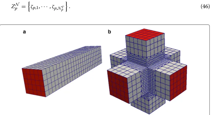
In the Offline stage, we already have some knowledge about the class of eigenproblems we will have to solve. We know the bilinear formsaandmcorresponding to the stiffness and mass operators. We have a predefined library of archetype components that will be allowed to be connected together at compatible ports to form bigger systems that will be considered in the Online stage. See Figure 3 for an example of library, and Figure 6 for an example of system obtained from component assembly. Note that each archetype component in the library is allowed to have some parametric variability.

For each port type corresponding to a possible connection between archetype compo-nents, we perform the following computations:

• Compute a set of port modes, possibly empirical modes as described in Section ‘Empirical mode construction’.

For each archetype component, we perform the following computations:

• Compute the harmonic extension of the port modes inside the archetype component

reference domain to get the interface functions.

• For each interface function, compute a reduced basis space for the bubble Eq. 16. Each RB space is tuned for the stiffness and mass operators, as well as the component parametric variability and the shiftσvariability.

• Precompute some component quantities used in (35), (36), that will be ready in the Online stage for system assembly.

Online stage

System assembly In the Online stage, we form a component assembly by instantiating Icomponents from our library of archetype components, and connecting them together. Several instantiated components can correspond to the same archetype component, but with possibly different parameter values. Each instantiated component i has a set of parameter valuesμi, and the whole system has a set of parametersμ= ∪i=1..Iμi. We also define a value ofσfor the whole system.

For each instantiated componenti, we perform the following computations:

• Compute the RB approximations of the bubble functions for parameter values(μi,σ).

• Compute the component stiffness and mass matrices (35), (36).

• Assemble the system (33) for parameter values(μ,σ), using the component matrices (35), (36) previously computed for each instantiated component.

Eigenvalue computation At this point, we now need to find the values ofσ for which the system (33) has a zero eigenvalue. We proceed by fixing an eigenvalue numbernand we then follow Algorithm 2 with toleranceδ1.

Algorithm 2

Pick an initial value forσ

Assemble the system (33) for(μ,σ)following Section ‘System assembly’ Compute thenth eigenvalueτn(μ,σ)of (33).

while|τn(μ,σ)|> δdo

Pick a new value ofσfollowing a search method (Brent) Reassemble the system (33) for(μ,σ)

Recomputeτn(μ,σ)

end while

Returnσ

Applying this algorithm forn = 1, 2, 3,. . . we can recover the first eigenvalues of the component assembly. In practice Brent’s method [21] applied to the search ofσsuch that _τn(μ,σ) = 0 converges in about 10 iterations, and there is only a single root for the functionσ→τn(μ,σ).

Once an approximationλn(μ)=σof the eigenvalue has been found, we obtain an asso-ciated eigenvector following (33). Note that we use a standard eigensolver from the SLEPc library [22] as a black box, hence we have no control on the eigenvector computation, especially when the eigenvalue multiplicity is two or more.

Remark 5.1. The parametric dependence comes into play in the Online stage when the RB bubble functions are computed, as they depend on(μ,σ). As a consequence, the resulting shifted system depends on(μ,σ), and also its eigenvaluesτn(μ,σ). The vector of

param-eters μ is chosen by the user for the whole system (material properties of the different components, geometry), whileσis automatically updated at each step of Algorithm 2: as a result, the RB bubble functions have to be recomputed at each step of Algorithm 2. In the end though, we obtain an approximationλn(μ)that depends only onμ, the “natural”

parameters of the original system. The user is then free to modify the system by choosing a different vector of parametersμ, and restart Algorithm 2.

Results and discussion Linear elasticity

We consider linear elasticity in a non-dimensional form: we nondimensionalize space with respect to a lengthd0 which will correspond to the beam width in the following,

we nondimensionalize the Young’s modulusE with respect to a reference valueE0, and

we nondimensionalize time with respect to

ρd0

E0 , whereρis the mass density. The non

dimensional linear elasticity free vibration equation then reads

−AU= ∂ 2_U

where Ais a linear second order differential operator in space andU(x,t) is the dis-placement vector. Assuming that the free vibration solution is of the form U(x,t) = u(x)cos(ωt), the problem is equivalent to solving the eigenproblem

Au=ω2u. (51)

In variational form, the operatorAcorresponds to the bilinear form [4]

a(w,v;μ)≡

(μ)Cijkl(μ)ij(w)kl(v) (52)

where we assume summation on repeated indices; a(·,·;μ) is defined on the space of admissible displacements V = v=(v1,v2,v3)|vi∈H1((μ));vi=0 on 0(μ)⊂∂(μ)}, andij(v) = 1₂(∂ivj+∂jvi). We will consider piecewise isotropic materials, in which case the coefficientsCijkl(μ)are functions of only two parameters at a given point in space: Poisson’s ratioνand Young’s modulusE. In the following we always fixν = 0.3, and allowE to vary, henceE is part of the vector of parametersμ. More precisely, the parametric dependence reads

Cijkl(μ)=

Eν

(1+ν)(1−2ν)δijδkl+ E

2(1+ν)(δikδjl+δilδjk). We also define the mass bilinear form

m(w,v;μ)≡

(μ)wivi. (53)

Note that there is also aμdependency coming from the possible geometrical variations, hence the notation(μ). If we define a mapping functionφμsuch that(μ)=φμ(ref),

for a reference domainref, then the mass bilinear form could also read:

m(w,v;μ)≡

ref

(wi◦φμ)·(vi◦φμ)|Jac(φμ)|, (54) and a similar expression could be obtained for the stiffness bilinear forma(·,·;μ).

The eigenproblem in variational form finally reads: findλ(μ)∈R>0andu(μ)∈Vsuch

that

a(u(μ),v;μ)= λ(μ)m(u(μ),v;μ), ∀v∈V, (55)

m(u(μ),u(μ);μ)= 1. (56)

Note thatλ(μ)=ω2(μ)– the eigenvalue is the frequency squared.

Simple component library

modes as described in Section ‘Empirical mode construction’; and we build a parameter independent preconditioner (necessary for the computation of) using parameter values E=0.5 ands=0.5.

Simple beam

We first present a simple example where we compare with beam theory to demonstrate that the FE resolution is adequate and that we capture the different modes. We connect eight beam components together, corresponding to a system with a vector of parameters μof dimension 16. By using the same values ofs=1 andE=1 for all beam components – or equivalentlyμ=1∈R16– we obtain a system corresponding to a uniform beam of square section, with thicknessd=1 and lengthL=40, and Young’s modulusE=1. As boundary conditions, we clamp this beam on both ends.

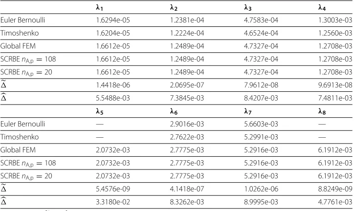
Table 1 presents the first eight eigenvalues obtained by different methods: Euler Bernoulli model [24], Timoshenko model [24], global FEM and SCRBE with and with-out port reduction (in which the beam is constructed as the concatenation of eight beam components). The eigenvalues (which we recall are the frequencies squared) are quite small as the beam is of large aspect ratio. The SCRBE results are obtained by connecting eight beam components together with length parameters = 1, using RB spaces of size N = 10; no port reduction corresponds tonA,p = Np = 108, and for port reduction we usenA,p =20 active port modes. The global FEM results are obtained using a global

mesh corresponding to eight beam component meshes stitched together, hence SCRBE and FEM are based on the same mesh and FE resolution.

We first observe that SCRBE does capture all the eigenvalues with their multiplicity: the eigenvalues corresponding to bending modes have double multiplicity because of the symmetry of the beam square section. We only report distinct eigenvalues in Table 1 but we show in Figure 4 the two non-collinear modes recovered by SCRBE for the first

Table 1 Eigenvalues for a clamped-clamped uniform beam of square section, with thicknessd=1 and lengthL=40

λ1 λ2 λ3 λ4

Euler Bernoulli 1.6294e-05 1.2381e-04 4.7583e-04 1.3003e-03

Timoshenko 1.6204e-05 1.2224e-04 4.6524e-04 1.2560e-03

Global FEM 1.6612e-05 1.2489e-04 4.7327e-04 1.2708e-03

SCRBEnA,p=108 1.6612e-05 1.2489e-04 4.7327e-04 1.2708e-03 SCRBEnA,p=20 1.6612e-05 1.2489e-04 4.7327e-04 1.2708e-03

1.4418e-06 2.0695e-07 7.9612e-08 9.6913e-08

5.5488e-03 7.3845e-03 8.4207e-03 7.4811e-03

λ5 λ6 λ7 λ8

Euler Bernoulli — 2.9016e-03 5.6603e-03 —

Timoshenko — 2.7622e-03 5.2991e-03 —

Global FEM 2.0732e-03 2.7775e-03 5.2916e-03 6.1912e-03

SCRBEnA,p=108 2.0732e-03 2.7775e-03 5.2916e-03 6.1912e-03 SCRBEnA,p=20 2.0732e-03 2.7775e-03 5.2916e-03 6.1912e-03

5.4576e-09 4.1418e-07 1.0262e-06 8.8249e-09

3.3180e-02 8.3262e-03 8.9995e-03 4.7761e-03

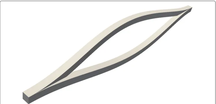
Figure 4 Two non-collinear eigenmodes corresponding to the first eigenvalue of double multiplicity.

eigenvalue. Regarding the beam models (Euler Bernoulli and Timoshenko), we observe that they do not capture some eigenvalues; these correspond to torsional modes that are not taken into account in Euler Bernoulli and Timoshenko models which consider only bending displacement. Note that for a beam with a square section, the bending and torsion is decoupled and the eigenmodes are either pure bending or pure torsion (see Figure 5). For the modes that are pure bending (λ1,λ2,λ3,λ4,λ6,λ7), we observe a good

agreement between all methods. Note that it is well known that Euler Bernoulli is better for long wavelength and/or slender beams; Timoshenko is better for shorter wavelength and/or shorter beams. Not surprisingly, the FE (and SCRBE) eigenvalues are closer to Euler Bernoulli for lower modes and closer to Timoshenko for higher modes. The SCRBE (with or without port reduction) and global FEM give results that have an actual relative difference less than 10−4. For the SCRBE without port reduction, we also give the relative error estimatein Table 1, which corresponds to the relative error between the SCRBE and the “truth” static condensation: it is at most 10−6, which confirms that the error intro-duced by RB is negligible. For the SCRBE with port reduction andnA,p=20, the relative

error estimate isand corresponds to the relative error between SCRBE with and with-out port reduction: it is abwith-out 10−2, which overestimates the actual relative error, but nonetheless indicates a very good agreement between SCRBE eigenvalues with and with-out port reduction. We also observe that the SCRBE does capture all the torsional modes. Note finally that the SCRBE eigenvalues are obtained using a root finding algorithm: in practice we set the tolerancea to 10−10 as this is a couple orders of magnitude smaller

than the RB relative error estimator, thus making the root finding error negligible with respect to RB error (and also port reduction error).

Bridge structure

We are now ready to consider larger systems with more complicated connections which will better exercise the RB and port reduction capabilities. Towards this end, we consider a system of 30 components, corresponding to a bridge structure. It is composed of 22 beam components and 8 connectors, hence the vector of parametersμfor this system is of dimension 52.

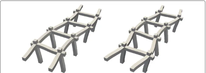
We first set the vector of parametersμsuch thatE = 0.5 ands = 1 for all compo-nents, and we show in Figure 6 the second and third eigenmodes for the corresponding system. In the following, we will provide systematic analysis of the RB and port reduction convergence and also performance of thea posteriorierror estimates.

We first show in Figure 7 the convergence of the first eigenvalue with respect to the size N of the RB spaces used for bubble approximations. Note that we did not compute the eigenvalue with the “truth” static condensation, because it would be very computation-ally intensive, hence the reference value forλis the value obtained with a global FEM, denotedλFEb. We observe that we obtain exponential convergence, hence we provide a significant improvement compared to standard CMS approaches. We also observe that the RB relative error estimatoris accurate – it overestimates the actual error by at most one order of magnitude; moreover, for a sufficiently largeN, the RB relative error estima-toris very small, hence justifying the fact that we can neglect the error due to RB error approximation when introducing port reduction.

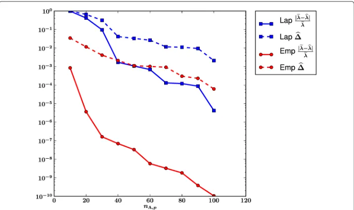
We now fixN=10 and consider port reduction. We show in Figure 8 the convergence of the first eigenvalue with respect to the number of port modes, for both the regular Laplacian modes and the empirical modes: the advantage obtained with the empirical modes is obvious, and we also observe thatdoes not converge as fast as the true error, which is due to the fact that it is only a linear function of the norm of the residual, as explained in Section ‘Port reduction error estimator’.

Finally, we briefly illustrate some component parametric variations made possible with SCRBE. We show in Figure 9 the third eigenmode for different parameter variations: we can modify some of the beam lengths (Figure 9a), or we can make one half of the bridge stiffer than the other (Figure 9b).

Figure 7 First eigenvalue convergence with respect to the sizeNof RB spaces.

Industrial example

In this last section, we apply our approach to a large industrial structure. In the following, we will first focus on computational performance (without using the error estimators that have already been presented in the previous section), and then we will illustrate the para-metric variability offered by our approach. Note that we will now consider linear elasticity in its dimensional form.

We consider here the shuttle part of a shiploader. A shiploader is a large structure (sim-ilar to a crane) used by mining companies to transport the minerals from trucks on the

Figure 9 Illustration of some variations of the vector of parametersμfor the bridge system. We show the third eigenmode for two different configurations.(a)For the middle beams,s₌0.7; for the beams adjacent to the middle beams,s₌1.3; for all other beams and all support beams,s₌1; andE₌0.5 everywhere.(b)

In the first half of the bridgeE₌2, in the second halfE₌0.5, and all the beams are of sizes₌1.

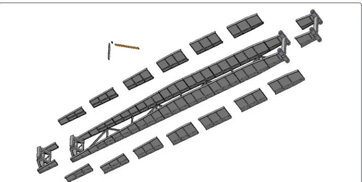
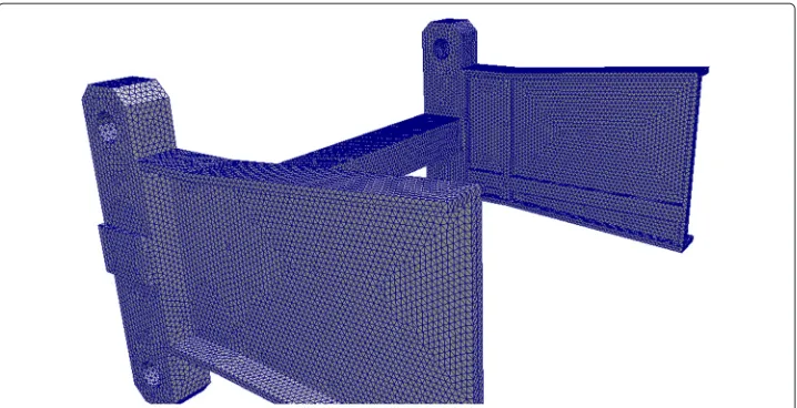
ground onto ships on the water. The shuttle is a subpart of the shiploader that can slide in and out, in order to vary the length and height of the structure, to accommodate for vary-ing shapes and sizes of the incomvary-ing ships. The shuttle is comparable to the lattice boom of a crane, and has a frame structure composed of a series of intermeshing steel rods, reinforced with some panels on the sides. The shuttle structure is shown in Figures 10 and 12.

The first goal of this section is to show the computational advantage of our method with respect to a classical Finite Element Method. The shuttle structure has a mesh composed of 430 000 nodes, and as a consequence the corresponding linear elasticity eigenproblem has 1.3 million degrees of freedom – we use first order elements and tetrahedral meshes. We show a part of the mesh for one of the components of the shuttle in Figure 11. For now, we consider the shuttle to be made of steel (Young’s modulus is 200GPaand mass density is 7850kg.m−3) and we impose clamping in four shuttle locations (at the bottom, in the back and the middle of the structure) corresponding to the case where the shuttle

Figure 11The shuttle is clamped at the locations indicated by the locks in the left picture. The next two pictures correspond to the first and fifth computed eigenmodes: we show the displacements superimposed on a translucid view of the original structure.

would slide halfway out of the complete shiploader structure. These clamping locations are indicated by the “lock” icons in Figure 12, where we also show the displacement for the first and fifth eigenmodes.

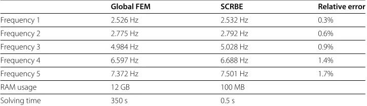
To solve the eigenproblem with SCRBE, we used RB spaces of dimension 20 on aver-age for the bubble approximations, and we used on averaver-age 15 empirical modes for each port at which components connect. The final Schur system is of size 1200, to be com-pared with the size of the original FE system which is 1.3 million. We report in Table 2 the first five natural frequencies (square root of the eigenvalues) obtained both with FE and SCRBE. We observe a very good relative error of at most 2%, despite the dramatic dimension reduction performed by SCRBE. With respect to computational time, SCRBE improves on FE by a factor 700, which is very significant and allows for quasi real-time computations. Another important gain for SCRBE is on memory usage: it requires only 100 MB to solve an eigenproblem that requires 12 GB with FE. It means that very large structures that are out of reach for FE can be considered with SCRBE. For instance, if we were to consider the full shiploader, there would be about 6 millions degrees of free-dom, and solving the eigenproblem with FE would not be possible on a regular desktop machine due to memory limitations, whereas it would be handled easily with SCRBE.