The influence of the unit commitment plan on the variance of electric power production cost

Spring 2018

The influence of the unit commitment plan on the variance of

The influence of the unit commitment plan on the variance of

electric power production cost

electric power production cost

Jinchi Li

Iowa State University, jinchi93qw@gmail.com

Follow this and additional works at: https://lib.dr.iastate.edu/creativecomponents Part of the Operational Research Commons, and the Power and Energy Commons

Recommended Citation Recommended Citation

Li, Jinchi, "The influence of the unit commitment plan on the variance of electric power production cost" (2018). Creative Components. 18.

https://lib.dr.iastate.edu/creativecomponents/18

production cost

by

Jinchi Li

A Creative Component paper submitted to the graduate faculty

in partial fulfillment of the requirements for the degree of

MASTER OF SCIENCE WITH CREATIVE COMPONENT

Major: Industrial Engineering

Program of Study Committee:

Sarah M. Ryan, Major Professor

Gary Mirka

Iowa State University

Ames, Iowa

TABLE OF CONTENTS

ABSTRACT . . . vi

CHAPTER 1. OVERVIEW . . . 1

1.1 Introduction . . . 1

1.2 Problem statement . . . 2

1.3 Literature review . . . 2

1.4 Model and power generating system . . . 3

1.5 Overview . . . 4

CHAPTER 2. MONTE CARLO SIMULATIONS . . . 6

2.1 Simulation model . . . 6

2.2 Results and comparison . . . 8

2.2.1 Test simulator functionality . . . 8

2.2.2 Input data . . . 8

2.2.3 Influence on total production cost . . . 11

2.2.4 Variance of production cost . . . 12

2.2.5 Normality of simulation results . . . 13

CHAPTER 3. APPROXIMATION BASED ON RENEWAL REWARD PROCESS . . . 21

3.1 Assumption . . . 21

3.2 Model . . . 21

3.2.1 The expected renewal cycle length . . . 22

3.2.2 The expected cost associated with a single renewal cycle . . . 23

3.2.3 The second moment of the cycle cost . . . 24

3.2.4 The cross moment of cost and renewal cycle length . . . 25

3.3.1 Discussion of test case . . . 26

3.3.2 Compare with simulation without two assumptions . . . 26

3.3.3 Simulation with assumptions . . . 27

3.3.4 Test on more unit commitment plans . . . 27

CHAPTER 4. CONCLUSION . . . 32

4.1 The influence of the unit commitment plan on the variance of total cost . . . 32

4.2 Other factors for future research . . . 32

4.2.1 The prediction of demand . . . 32

4.2.2 A generalized approach to the simplified model . . . 33

LIST OF TABLES

2.1 Comparison of results listed in Ryan (1997) and results from this simulator 8

2.2 Net load (highest probability) . . . 10

2.3 Generating units . . . 16

2.4 Mean of total production cost ($) from simulation . . . 17

2.5 Total production cost variance ($2) from simulation . . . 17

2.6 Production cost variance slopes (σ2/T L) from simulation . . . 17

3.1 Calculation results for proportion of time that one specific unit failed (F P1j) 30 3.2 Approximation result . . . 30

3.3 Variance estimates from simulation with and without assumptions ($2_{) . . 31}

A.1 Commitment plan from SP CVaR 02 . . . 34

A.2 Commitment plan from SP CVaR 002 . . . 35

A.3 Commitment plan from SP CVaR 0002 . . . 36

A.4 Commitment plan from RO U1 01 . . . 37

A.5 Commitment plan from RO U1 05 . . . 38

LIST OF FIGURES

2.1 Net load cycles (20 scenarios) . . . 9

2.2 Net load cycle (high-probability scenario) . . . 9

2.3 Net load and total capacity committed for different commitment plans . . . 11

2.4 The minimal dispatch cost(without failure) from SP CVaR and RO U1 . . . 12

2.5 Simulation results: mean cost comparison . . . 13

2.6 Simulation result: histogram of production cost (2016 hr) . . . 14

2.7 Simulation result: histogram of production cost (6048 hr) . . . 15

2.8 Simulation result: histogram of production cost (8064 hr) . . . 18

2.9 Simulation result: histogram of production cost (10080 hr) . . . 19

2.10 Simulation result: histogram of production cost (12096 hr) . . . 20

3.1 A renewal cycle . . . 21

3.2 A time segment . . . 23

3.3 Simulation results for other unit commitment plans . . . 28

ABSTRACT

In electricity production systems, generating unit failures will result in higher electricity

pro-duction cost. For a system operator, the variance of propro-duction cost is an important factor for

choosing the proper commitment plan, because generating unit failures require a much more

ex-pensive unit to replace their electricity production task. Unit Commitment (UC) seeks a thermal

generator commitment schedule that meets the net electricity demand in the most cost-effective

way while satisfying operational constraints on both transmission and generation systems. The

un-expected, extremely high operational cost is undesirable for system operators. The production cost

variance could be helpful when decision makers try to select a commitment plan with low risk in its

operational cost. In this project, we focus on the behavior of production cost variance for different

commitment plans under a simplified model of an electric production system. In the simplified

system, the warm up and shut down periods of generating units are ignored. First, a simulation

model and an approximation method are built to estimate the production cost variance of this

sim-plified system. Then, the influence of the commitment plan is observed based on simulation results.

After that, the performance of both estimation approaches is tested using commitment plan data.

The contribution of this project is that we incorporate the influence of the commitment plan into

the production cost variance calculation and propose a potential approach for commitment plan

evaluation. In the proposed approach, the decision makers could use the approximation method to

select some good commitment plans from a large set of commitment plans and use the simulation

CHAPTER 1. OVERVIEW

1.1 Introduction

The deepening penetration of renewable energy helps society to solve the problems of limited

quantities of fossil fuel and carbon dioxide emissions. However, it also brings a new problem, as

most of the renewable energy sources are associated with high variability in energy production.

For example, the wind power can be very high on some days but very low on the next days,

or solar power can be high on a sunny day but low when it is raining. The International Energy

Outlook 2017 from U.S Energy Information Administration (EIA) predicts the growth of electricity

consumption and the growing share of renewable energy in the next 23 years [1]. To deal with the

variability in electricity supply, people could increase the electricity storage units. However, an

important property of electricity is that it cannot be stored easily. Large-scale storage of electricity

is very expensive. So, electricity system operators should try to meet the current net load as much

as they can. Net load is defined as the difference between the electricity demand and the output

of renewable energy production. If there is a generating unit failure at the same time as high net

load, then the system operator needs to increase production from expensive generators or to use

expensive storage units. In those extreme situations, the production cost will skyrocket. Those

high costs threaten the daily operation of electricity production systems. This concern can be

addressed by considering and evaluating the risk associated with a given unit commitment plan.

Unit commitment seeks for generator commitment schedules (unit commitment plans) that meet

the net electricity load in the most cost-effective way while satisfying operational constraints on

1.2 Problem statement

The risk of a unit commitment plan is evaluated by estimating the production cost of an

electricity generation system following this unit commitment plan in unexpected situations. An

unexpected situation could be a failure of scheduled generating units in the production system.

Different unit commitment plans will react differently in those unexpected situations. Evaluating

the performance of some unit commitment plans would be helpful to select one with acceptable

operation costs in those situations. To assess the risk numerically, the variance of the production

cost for a given unit commitment plan is the focus of this project.

1.3 Literature review

There already exist several numerical measures of risk which are used in UC. Loss of Load

Probability (LOLP), Value at Risk (VaR) and Conditional Value at Risk (CVaR) are three different

risk measures. LOLP is the most widely used measure for evaluating system-wide risk. However,

LOLP also requires significant computational power. On the other hand, those measures like

CVaR, which have been introduced more recently, are more computationally efficient. CVaR is the

expected loss (cost) for the worst cases with probability lower than a given threshold value. More

detail about these different risk measures can be found in Zheng’s review of unit commitment [2].

Compared with CVaR, variance is describing production cost from a more general perspective, and

variance along with the mean can also be used to calculate the CVaR of a normally distributed

random variable. Over a long time period, the production cost is asymptotically normal according

to central limit theory.

There are some previous researches about the variance associated with electricity production

systems. In 1995, Shih verified the asymptotic behavior of electric power generation cost using

simulation [3] and Shih et al. also developed a method to utilize the state space of Markov chain

to calculate the asymptotic mean and variance of production cost [4]. In 1997, Ryan presented

an approximation method for variance of electric power production cost based on renewal reward

generat-ing units and electric demand by incorporatgenerat-ing time series analysis for electric demand and Monte

Carlo simulation of the generating units’ availability [6]. Their research suggested that the load

variability plays an important role in the variation of production cost. In 2016, Kazemzadeh’s

research applied the approximation method from Ryan to the estimation of CVaR [7]. The

ap-proximation method for CVaR introduced in Kazemzadeh’s research can be used when asymptotic

assumption is appropriate. However, those previous studies did not examine the influence of the

unit commitment plan to the production cost variance.

1.4 Model and power generating system

Assume there are n generators (generating units) in a given electric generation system. For

each generation unit jthere is a capacity cj (in MW) and a variable production costdj (in $/MW

h) associated with it. The list of units is ordered as d1 ≤ d2... ≤ dn. The times between unit

state changes are modeled as exponentially distributed random variables with failure rate λj and

repair rate µj. The minimum up and down time of the generating units are ignored in this model,

but they are considered in the unit commitment problem. The minimum cost to satisfy a given

electricity demand (net load) is obtained by dispatching the least expensive unit available first.

Dispatching means to assign total load to generation units.

The variation from electricity demand and the uncertainty of generating unit availability are

two important factors in estimating electricity production cost variance. To capture the variation

in electricity demand, the estimation of the generation system’s net electricity demand (DLE), also

called the net load for the system, is used. The net load estimation seeks to predict the future

load from historical data. In these predictions, the historical data is not just about the electricity

demand. Weather data is also used in many net load estimation models. Net load estimation is

a hard task because of the complexity of the electricity market. To capture the variation in the

production system, the estimation of the state of a production system (SPE) is developed. In

time t, the state of generating unit j reflects whether unit j is available for production at that

state estimation of a production system is dealing with the combination of both the deterministic

schedule and the stochastic availability of generation units. A vector S is used to represent the

state of the production system at time t (hr). A variable Sj in this vector will be zero if either

unitj is scheduled to be down or is failed. On the other hand, a vectorI is used to represent only

the condition of generating units in the system. A variable Ij is zero if unit j is failed and one

otherwise.

By combining DLE and SPE, a production cost is estimated. For a given DLE and SPE in a

time period, the corresponding part of the production cost is calculated by assigning load to units

following the unit selection rule discussed previously in this section. For simplification purposes,

the failure of the generator unit can be treated as independent of the unit’s operational status.

With this simplification, the demand side of system will not influence the failure of a generator

unit in our model. Thus DLE and SPE can be done separately. The unit commitment plan will

directly influence the state of the production system in a given time period. For some time periods,

the old version of cost effective dispatch solutions which do not consider the unit commitment

plan will be no longer feasible. In those time periods, the system has to dispatch more electricity

production on more expensive units compared with the old version. As a result, this increases the

total production cost as well.

1.5 Overview

To estimate the variance of electricity production with unit commitment plans, both the Monte

Carlo simulation approach and an approximation approach based on renewal reward processes

are considered in this project. Some of the results also appear in [8]. This paper will go over

those procedures considered in simulation after the introduction to the input data of simulation

in Chapter 2. The approximation method adapted from Ryan’s method will be discussed with

the derivation process in Chapter 3. The dataset from Kazemzadeh will be used as a test case to

compare these two approaches. The result for a test case from both the simulation approach and

be given in Chapter 4 as well as some potential topics which interest us throughout the research

CHAPTER 2. MONTE CARLO SIMULATIONS

2.1 Simulation model

The result from a simulation program built in MATLAB was used to test the influence of unit

commitment plan on electricity production cost variance and the hypothesis of normal distribution.

The normal distribution is a crucial factor for the connection between variance and CVaR. Since

the failure of a generating unit does not happen very often, it is very likely that for many runs

there will be no failure of any unit. However, the time generating units is failed is the time that

we want to focus on. To deal with this, the time horizon for simulation was extended by repeating

the new load patter of a given day multiple times.

The input parameters for the simulation include: the new load profile; unit commitment (UC);

time horizon considered (TL); repair rate (µ) and failure rate (λ); the capacity (c) and variable

cost (d) of the generating units; and a penalty cost for not satisfying net load. The warm-up and

shut-down times for the generating units were ignored in our model, but they have been taken care

of in the UC. The program will output the expected value and standard deviation for electricity

production cost for the given electricity production system. In addition, the a goodness-of-fit test

result will also be provided for the hypothesis that production cost is normally distributed.

The way to decompose the problem discussed in the previous section can be treated as a

guideline for the simulation. The initial state of the power generation system is determined by

the forced outage rate of each unit pj. The forced outage rate can be calculated by λj/(λj+µj)

which represents the long-run proportion of time that unitj is unavailable due to the unexpected

failure of the unit itself. Then, the program generates a time point for each generating unit when

will change its state from failure rate and repair rate. The state of a generating unit represents

whether it is ready to generate electricity power. At the same time, the system state will change

units (SCF). The unit commitment plan can cause system state changes as well. Different from

the changes due to generating units, those system state changes due to the unit commitment plan

(SCP) are predetermined. In our simulation process, the SCF is captured by the simulation of

generators’ failures while the SCP is embedded in the calculation of production cost for each time

segment. In our model, the net load has been considered as a value that varies only hourly. This

pattern is consistent with those unit commitment plans which schedule the generators (generating

units) every hour.

In our simulation model, the time point that a generating unit’s failure happens is marked as

SCFT. The time points that the system state changes due to the unit commitment plan (SCPT)

are at the beginning of every demand hour. Both SCPT and SCFT are considered as the time

points in which the system change its state (CT). From a simulation point of view, CT determines

when the production cost calculation will be different. The simulation is all about figuring out the

next CT and calculating the cost between two CTs. Those steps are also listed in Algorithm1.

Algorithm 1 Monte Carlo Simulation

while n <total number of trials [T S]do . Do simulation multiple trials Step 1. Initialize two variables: t= 0, Cost= 0

Step 2. Generate initial value forI according to their force outage rate (p)

whilet6> T L do . Simulate until reach end time

Step 3. Generate a time (t∗) for each machine when it changes state (repairing finishes or failure happens) according to I.

Step 4. Set tnext= the closest next time point where a machine state will change or the

demand will change. . Figure out next CT

Step 5. Calculate the cost between (t, tnext) and add it to Cost. . Calculate cost in CT

Step 6. Change I according to step 4, and updatet=tnext end while

Step 7. Record theCost for this trial

end while

Step 8. Calculate variance and mean for all the Cost and perform K-S test

return the statistic result from Step 8 . Output from simulation

When testing the normality of the simulation result for production cost, both Pearson’s

chi-square test and the Kolmogorove-Smirnov (K-S) test are commonly used methods. However, the

The number of groups, g, is a crucial factor for the result of this test, but choosing a good g is

very hard. Thus, the K-S test is the one used as our criterion to determine the normality of the

simulation result. The Kolmogorov-Smirnov test in statistics is used to test the null hypothesis

that the empirical Cumulative Distribution Function (CDF) is close to the hypothesized CDF. Its

test statistic is based on the maximum absolute difference between the two CDFs.

2.2 Results and comparison

2.2.1 Test simulator functionality

The functionality of the simulator was tested on the data set from Ryan’s paper [5]. Since the

model in [5] did not incorporate a UC plan, a unit commitment plan which schedules every unit

to be available at all time periods was used in this subsection. For each TL value, the simulator

simulated and recorded results 1000 times. The mean and standard deviation (square root of

variance) for the simulation results are calculated and shown in Table 2.1. In this testing, the

standard deviation was used to be consistent with the result format in [5]. As shown in Table 2.1,

this simulator gets results close to the results in [5] when using same dataset.

Table 2.1 Comparison of results listed in Ryan (1997) and results from this simulator

mean ($) standard deviation ($) TL(hr) Ryan this simulator Ryan this simulator

168 9.300E+06 9.32E+06 2.600E+06 2.501E+06 672 3.720E+07 3.720E+07 6.400E+06 6.490E+06 2016 1.120E+08 1.113E+08 1.200E+07 1.212E+07

After testing simulator functionality, this simulator is ready for the test case from Kazemzadeh’s

paper [7].

2.2.2 Input data

The numerical experiments are based on Kazemzadeh’s calculation for net load in [7]. Kazemzadeh

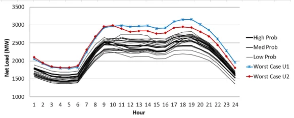
and 38 transmission lines [9]. In [7], there are 20 scenarios which are constructed from 365 scenarios

using the fast forward selection algorithm as shown in Figure 2.1. The 20 scenarios include one

with a probability of 0.58 and three with probabilities of 0.09, 0.11, and 0.13, and the remainder

with probability lower than 0.05. They correspond to the High-, Medium- and Low- probability in

Figure 2.1.

Figure 2.1 Net load cycles (20 scenarios)

For simplification purposes, the numerical testing is focused on the net demand of the

High-probability scenario (Figure2.2). The numerical values for this net load data are provided in Table

2.2.

Figure 2.2 Net load cycle (high-probability scenario)

The data for production system is in Table2.3.

The simulation tests two kinds of different unit commitment plan results from Kazemzadeh’s

paper. These unit commitment plans are generated from a stochastic program model with CVaR

(SP CVaR in short) and the Robust Optimization with uncertainty set (RO U1). Kazemzadeh

Table 2.2 Net load (highest probability)

Period Net load required (M W h)

1 1800

2 1722

3 1637

4 1608

5 1608

6 1637

7 2028

8 2337

9 2526

10 2446

11 2448

12 2421

13 2422

14 2420

15 2371

16 2396

17 2529

18 2556

19 2558

20 2452

21 2324

22 2123

23 1862

24 1596

specification refers to SP CVaR with gamma=0.002 (SP CVaR 002) and RO U1 refers to RO U1

with delta=0.05 (RO U1 05). The section where all six unit commitment plans is discussed will

be using the same format to name those unit commitment plans. The case without considering

the unit commitment plan is called the default plan. In the default plan, every generating unit is

scheduled to be available in every hour. The default plan is considered in order to figure out the

influence of introducing the unit commitment plan. The unit commitment plans can be founded in

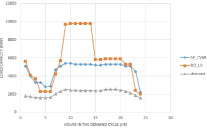
Figure 2.3 Net load and total capacity committed for different commitment plans

The total capacity unit committed for every hour is plotted in Figure 2.3. It is clear that the

RO U1 unit commitment plan schedules generators with much higher total capacity between hours

eight and fifteen. This coincides with the property of two unit commitment plans described in

Kazemzadeh’s paper where the Robust Optimization method tries to guarantee the performance

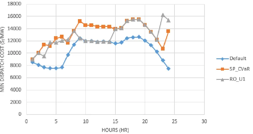
of the system in the worst scenario. The minimal dispatch cost for every unit commitment plans

(assuming no failure) is shown in Figure2.4. From this figure, the total production cost of two unit

commitment plans should not have much difference in the long run.

2.2.3 Influence on total production cost

The expected production cost with a unit commitment plan should be higher than with the

default plan. The reduced number of units available for a given hour will potentially require using

more expensive units than with the default plan to satisfy net demand. This is the case when the

Figure 2.4 The minimal dispatch cost(without failure) from SP CVaR and RO U1

generating units ready for production. The cost required for keeping generating units available is

deterministic for a given commitment plan. Our goal is to compare the variance of production cost;

we choose to ignore those deterministic parts for now.

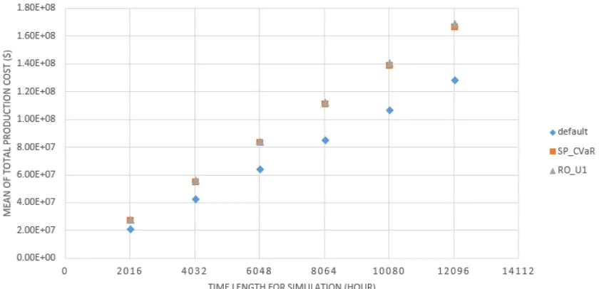
Figure2.5shows the linear relationship between expected cost and time length in consideration.

Table2.4 shows the mean of total production cost that results from the simulation. Just as what

was expected, the expected production costs are about the same for SP CVaR and RO U1.

2.2.4 Variance of production cost

The simulation results show that the increase in variance tends to have the constant slope over

the long run. The slope of variance is estimated by dividing TL into variance. This coincides with

the simulation experiment result from Shih [3]. At the same time, both SP CVaR and RO U1

commitment plan have greater variance than the default plan. The variance slope of RO U1 is

Figure 2.5 Simulation results: mean cost comparison

2.2.5 Normality of simulation results

When applying the simulation method with TS = 1000 and TL = 12096 hrs, running a unit

commitment simulation takes more than half an hour. The simulation method would require

much more computation power and increase the time to finish computation when the size of the

focused system increased. The approximation method could be a good approach to handle those

more complex systems. The approximation methods from both Shih [4] and Ryan [5] make the

assumption about the asymptotic property of the total cost. Thus, we need to test if this assumption

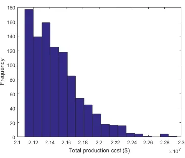
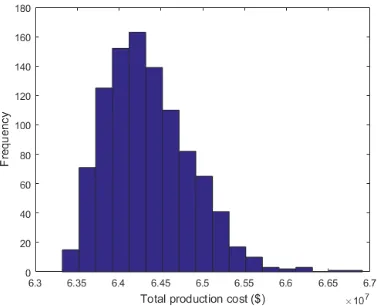
is appropriate for our system. Before running any tests for normality, the histogram of the default

unit commitment plan was studied to explore how the shape of the production cost distribution is

changing with TL. Figures2.6,2.7,2.8,2.9and2.10show how the distribution of total production

cost approaches a normal distribution as TL increases.

Instead of looking at the histogram of those simulation results one by one, the K-S test is

used for testing the normality for all the simulation results. With a significant value of 5%, the

hypothesis test result for the K-S test from simulation shows that those results with the default

Figure 2.6 Simulation result: histogram of production cost (2016 hr)

the test when the time horizon reaches 4032 hr, but those results with RO U1 fail to pass the K-S

test even when TL reaches 12096 hr. Thus, those unit commitment plans can influence the time

Table 2.3 Generating units

unit capacity (M W) MTTF (hours) MTTR (hours) d ($/M W h)

1 1000 1440 160 4.5

2 900 1300 150 5

3 700 1200 130 5.5

4 600 1100 110 5.75

5 600 1100 110 5.75

6 500 1150 110 6

7 500 1150 110 6

8 500 1150 110 6

9 400 1100 90 8.5

10 400 1100 90 8.5

11 400 1100 90 8.5

12 400 1100 90 8.5

13 400 1100 90 8.5

14 300 1000 70 10

15 200 850 48 14.5

16 200 850 48 14.5

17 200 850 48 14.5

18 200 850 48 14.5

19 200 850 48 14.5

20 100 600 48 22.5

21 100 600 48 22.5

22 100 600 48 22.5

23 100 600 48 22.5

24 100 600 48 22.5

25 100 600 48 22.5

26 100 600 48 22.5

27 100 350 12 44

28 100 350 12 44

29 100 350 12 44

31 100 350 12 44

Table 2.4 Mean of total production cost ($) from simulation TL(hr) default SP CV aR RO U1

2016 2.15E+07 2.78E+07 2.83E+07 4032 4.29E+07 5.56E+07 5.64E+07 6048 6.44E+07 8.34E+07 8.46E+07 8064 8.58E+07 1.11E+08 1.13E+08 10080 1.07E+08 1.39E+08 1.41E+08 12096 1.29E+08 1.67E+08 1.69E+08

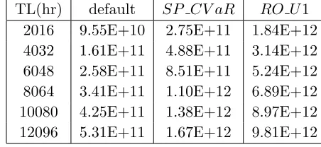
Table 2.5 Total production cost variance ($2) from simulation TL(hr) default SP CV aR RO U1

2016 9.55E+10 2.75E+11 1.84E+12 4032 1.61E+11 4.88E+11 3.14E+12 6048 2.58E+11 8.51E+11 5.24E+12 8064 3.41E+11 1.10E+12 6.89E+12 10080 4.25E+11 1.38E+12 8.97E+12 12096 5.31E+11 1.67E+12 9.81E+12

Table 2.6 Production cost variance slopes (σ2/T L) from simulation TL(hr) default SP CV aR RO U1

CHAPTER 3. APPROXIMATION BASED ON RENEWAL REWARD

PROCESS

3.1 Assumption

Different from the system simulated, Ryan’s approximation method [5] was built with two more

assumptions. The assumptions will be listed below with some explanation.

Assumption one: No more than one scheduled generating unit will fail at one time period.

With this assumption, the changing of the generating unit availability state (I) is a renewal process.

In probability theory, a counting process with i.i.d times between successive events is called a

renewal process.

Assumption two: The failure happens at the beginning of a load cycle.

With this assumption, the calculation of production cost associated with a given time segment is

simplified.

3.2 Model

In this approximation method, the total production cost in TL is calculated based on the

production cost of renewal cycles. Figure3.1shows a single renewal cycle with length T.

Figure 3.1 A renewal cycle

In time segmentX, all the production units scheduled are available and total cost corresponding

to this segment isU. For any instant of timetinX, the cost functionu(t) is used to represent the

cycle where one generating unit j is unavailable and the cost for this period is V. In the same

manner, the cost functionvj(t) is used to represent the cost for instanttinY when generating unit

j is unavailable. We useZ to represent the total cost associated with a single renewal cycle, where

Z =U +V.

Based on previous research, the increase of production cost variance is in proportion to the

increase of TL. In the long run, how fast the variance increases as TL increases (also called the

slope of the variance) will dominate the total variance. To estimate the variance of total production

cost, the slope of the variance (a) is our main focus. A study from Brown and Solomon [10] shows

that the variance’s slope of the total reward can be separated into three parts. The formula shown

below is the equation for parameterawritten in the form of parameters related to a renewal cycle

from [5].

a= E(T

2_)E(Z)2

E(T)3 −

2E(ZT)E(Z)

E(T)2 +

E(Z2)

E(T)

The next few subsections will focus on calculations for all the parameters needed for this formula.

Most of these equations used are coming from [5]. In this paper, some extra explanation and

deviations are added to make it easier to understand.

3.2.1 The expected renewal cycle length

This section focuses on the expected length of a renewal cycle E(T) and the expected length

squared of a renewal cycleE(T2). Since the length ofY is independent of the length of X, we can write the equations below:

E(T) =E(X) +E(Y)

E(T2) =E(X2) + 2E(X)E(Y) +E(Y2)

By the property of exponential distribution, X is exponentially distributed with parameter Λ =

P

jλj and Y is exponentially distributed withµj accordingly. When a generator fails, it happens

to be machine j with probability λj/Λ. So, the expected values for X and Y can be found by

E(X) = 1/Λ E(X2) = 2/Λ2 E(Y) =P j

λj

Λµj E(Y

2_{) =E}

J[E(Y2|J)] =P_{j µ}2λ2j

jΛ

3.2.2 The expected cost associated with a single renewal cycle

This section focuses on the calculation related to the expected cost when all scheduled generators

are available, E[U], and the expected cost when one machine is failed, E[V], in a single renewal

cycle. For computational convenience, time segments X and Y are treated as the combination of

several demand cycles with length ∆ and a remainder part with lengthR, whereX =R+K∆ and

Y =Rj +Kj∆. Figure 3.2shows how a time segment is divided into ∆ andR .

Figure 3.2 A time segment

By some derivations based on the exponential distribution, the expected number of load cycles

isE[K] = e

−Λ∆

1−e−Λ∆ and the density function ofR isf(r) =

Λe−Λr

1−e−Λ∆ when no generator is failed.

E[U] can be written in the formula shown below:

E[U] =E[K]E[U|T = ∆] +E[U|T =R] = e

−Λ∆

1−e−Λ∆

Z ∆

0

u(t)dt+E Z R

0

u(t)dt

The term E Z R

0

u(t)dt

can be treated as a cumulative conditional expected value. Using Ui

to represent

Z i

0

u(t)dt, the term E Z R

0

u(t)dt

can be written as follows:

E Z R

0

u(t)dt = Z ∆ 0 Z r 0

u(t)dt f(r)dr

=

∆−1

X

0

Z i+1 i

Z r

0

u(t)dt f(r)dr

=

∆−1

X

0

Z i+1 i

(ui+1(r−i) +Ui)

Λe−Λr

1−e−Λ∆dr

Similarly, the calculation for E[V] has the same structure:

E[V] =P(J =j)E[V|J =j] = λj Λ

e−µj∆ 1−e−µj∆

Z ∆

0

vj(t)dt+E Z Rj

0

vj(t)dt

(3.2)

UsingVj,i to represent Z i

0

vj(t)dt, theE Z Rj

0

vj(t)dt

can be written as follows:

E Z Rj

0

vj(t)dt = Z ∆ 0 Z r 0

vj(t)dt fj(r)dr

=

∆−1

X

0

Z i+1 i

Z r

0

vj(t)dt fj(r)dr

=

∆−1

X

0

Z i+1 i

(vj,i+1(r−i) +Vj,i)

µje−µjr

1−e−µj∆dr

(3.3)

The expected cost associated with single renewal cycle can be calculated by adding those two

expectations togetherE(Z) =E[U] +E[V].

3.2.3 The second moment of the cycle cost

To compute E(Z2_{), the missing part is justV ar(Z) according to the equation below:}

E(Z2) =V ar(Z) +E[Z]2

V ar(Z) =V ar(U) +V ar(V)

V ar(U) =V ar(K)

Z ∆ 0

u(t)dt 2

+V ar Z R

0

u(t)dt

Since K is geometrically distributed,V ar[K] = e

−Λ∆

(1−e−Λ∆₎2 and

V ar Z R

0

u(t)dt

=E Z R

0

u(t)dt2

−E Z R

0

u(t)dt 2 , where: E Z R 0

u(t)dt2 = Z ∆ 0 Z r 0

u(t)dt 2

f(r)dr

=

∆−1

X

0

Z i+1 i

Z r

0

u(t)dt2f(r)dr

=

∆−1

X

0

Z i+1 i

"

ui+1(r−i) +

i X k=0

uk #2

Λe−Λr

1−e−Λ∆dr

The calculation forV ar(V) follows the same structure:

V ar(V) =Ej[V ar(V|J)] +V arj[E(V|J)]

Ej[V ar(V|J)] = X

j λj

Λ

(

V ar(Kj) Z ∆

0

vj(t)dt 2

+V ar Z Rj

0

vj(t)dt )

, (3.5)

where:

V ar(Kj) =

e−µj∆ (1−e−µj∆₎2

V ar Z Rj

0

vj(t)dt

=E Z Rj

0

v2_j(t)dt

−E Z Rj

0

vj(t)dt 2

E Z Rj

0

v2_j(t)dt = Z ∆ 0 Z r 0

vj(t)2dt fj(r)dr

=

∆−1

X

0

Z i+1 i

Z r

0

vj(t)2dt fj(r)dr

=

∆−1

X

0

Z i+1 i

(v_j,i2 ₊₁(r−i) +

i X k=0

v2_j,k) µje

−µjr 1−e−µj∆dr

V arj[E(V|J)] = n X j=1

λj

ΛE(V|J =j)

2₋   n X j=1 λj

ΛE(V|J =j)

 

2

(3.6)

3.2.4 The cross moment of cost and renewal cycle length

The expected product of Z and T is:

E(ZT) =E(U X) +E(U)E(Y) +E(V Y) +E(U)E(X)

E(U X) =

∆E(K2) +E(K)E(R) Z ∆

0

u(t)dt+ ∆E(K)E Z R

0

u(t)dt +E R Z R 0

u(t)dt

,

where E[K2] = e

−Λ∆_{(1 +e}−Λ∆₎

(1−e−Λ∆₎2 ,E[R] =

1−(Λ∆ + 1)e−Λ∆

Λ(1−e−Λ∆₎ and

E

R Z R

0

u(t)dt

=

∆−1

X

0

Z i+1 i

Z r

0

ru(t)dt f(r)dr

=

∆−1

X

0

Z i+1

i

(ui+1(r2−ir) +Uir)

Λe−Λr

1−e−Λ∆dr

Similarly,E(V Y) can be found, usingE[K_j2] = e

−µj∆_{(1 +e}−µj∆₎

(1−e−µj∆₎2 andE[Rj] =

1−(µj∆ + 1)e−µj∆ µj(1−e−µj∆)

,

as

E(V Y|j=J) =∆E(K_j2) +E(Kj)E(Rj)

Z ∆

0

vj(t)dt+∆E(Kj)E Z Rj

0

vj(t)dt

+E

Rj Z Rj

0

vj(t)dt

3.3 Results and comparison

3.3.1 Discussion of test case

In this results section, the approximated method will be applied to the same test case as in

Section 2.2. Before applying the approximated method, we check if assumption one is appropriate

for this case. The forced outage ratepis used to calculate the total proportion of time for one unit

failed (F P1) or no unit failed (F P0). F P1j is the proportion of time when only unit j is failed.

The formulas forF P1,F P1j and F P0 are listed below:

F P0 =

n Y j=1

(1−pj) ; F P1 = n X j=1

pj Y i6=j

(1−pi) ; F P1j =pj Y i6=j

(1−pi)

In our test case, the F P0 value is 0.104494. This means there is at least one unit failed most of

the time. The calculation results for F P1j are shown in Table3.1. F P1j is the proportion of time

for only unit j is failed. Summing up the proportion of time for each unit gives F P1 = 0.2455.

Thus, this approximation method seems not well suited for this test case. However, we still apply

this approximation method to see the impact of violating this assumption.

Assumption two is discussed in Section 3.3.3.

3.3.2 Compare with simulation without two assumptions

The approximation approach has been implemented in MATLAB. The calculation result in

Table 3.2 has expected total production which is very close to the mean cost from the simulation

approach. Different from the simulation result without those two assumptions, the approximation

discussed. This means that the approximation method developed will lose some accuracy compared

with the simulation approach, while we want to assess the difference between two unit commitment

plans. However, it could be potentially useful for selecting some outstanding unit commitment plan

before the implementation of the time consuming simulation method.

3.3.3 Simulation with assumptions

When considering the influence of these two assumptions, a simulation model is developed to test

out the two cases where assumptions are included progressively. Table 3.3 shows the results from all

cases. When we incorporate only assumption one, the variance from both unit commitment plans

have significant changes. The ratio between production cost variance from RO U1 and SP CVaR

changes from 6 to 2.4. This shows that this assumption could have different influence to production

cost with different unit commitment plans. When considering assumption two, the variance of

production cost is increased by 34% with both unit commitment plans while the ratio between

production cost variance from RO U1 and SP CVaR stays the same at around 2.4. An interesting

fact is that the simulation method produces a result very close to the approximation method’s

when simulated with both assumptions.

From the previous discussion and simulation result, the assumption one is the cause for the ratio

difference between two approaches. There could be some further research about the influence of

relaxing assumption one in approximation method. For example, when can we accept assumption

one?

3.3.4 Test on more unit commitment plans

Even though the approximation method does not reflect the simulation result very closely, it

can still be useful when there remains some relationship between the unit commitment plans. To

check out this idea, both the approximation method and the simulation method are applied to the

other four unit commitment plans from Kazemzadeh’s research. Figure3.3shows the slope of mean

calculated by applying linear regression on all 6000 simulation results (one thousand for each TL).

At the same time, the confidence interval for each slope value is calculated and shown in Figure

3.4. The calculation of the confidence interval for variance is done by the Jackknife re-sampling

method [11]. For each data point, our program calculated a ”variance” value without this data

point. Then we treat those ”variance” values as our data points to calculate the confidence interval.

Unit commitment plans RO U1 01 and RO U1 10 are distinguishable from other unit commitment

plans. As seen in Figure 3.4, none of those unit commitment plans have both smaller mean and

standard deviation than RO U1 10 and RO U1 10. Those two interesting unit commitment plans

are also distinguishable in Figure 3.5. Following the same rule, the decision maker would choose

those two unit commitment plans. If people could choose more unit commitment plans based

on Figure 3.5, it would be even less likely that they will miss those two unit commitment plans.

This suggests that the approximation method could be useful to select some relatively good unit

commitment plans which helps to save some computational power in the simulation stage.

Figure 3.4 Simulation results for other unit commitment plans (with confidence intervals)

Table 3.1 Calculation results for proportion of time that one specific unit failed (F P1j)

unitj pj 1-pj F P1j

1 0.1000 0.9000 0.0116

2 0.1034 0.8966 0.0121

3 0.0977 0.9023 0.0113

4 0.0909 0.9091 0.0104

5 0.0909 0.9091 0.0104

6 0.0873 0.9127 0.0100

7 0.0873 0.9127 0.0100

8 0.0873 0.9127 0.0100

9 0.0756 0.9244 0.0085

10 0.0756 0.9244 0.0085

11 0.0756 0.9244 0.0085

12 0.0756 0.9244 0.0085

13 0.0756 0.9244 0.0085

14 0.0654 0.9346 0.0073

15 0.0535 0.9465 0.0059

16 0.0535 0.9465 0.0059

17 0.0535 0.9465 0.0059

18 0.0535 0.9465 0.0059

19 0.0535 0.9465 0.0059

20 0.0741 0.9259 0.0084

21 0.0741 0.9259 0.0084

22 0.0741 0.9259 0.0084

23 0.0741 0.9259 0.0084

24 0.0741 0.9259 0.0084

25 0.0741 0.9259 0.0084

26 0.0741 0.9259 0.0084

27 0.0331 0.9669 0.0036

28 0.0331 0.9669 0.0036

29 0.0331 0.9669 0.0036

30 0.0331 0.9669 0.0036

31 0.0331 0.9669 0.0036

32 0.0331 0.9669 0.0036

Table 3.2 Approximation result

UC Plan Expected cost ($) at TL=2016 Varianceσ2_($2_{) at TL=2016 Slope of σ}2_($2_/hr)

SP CVaR 2.66E+07 8.39E+10 4.16E+07

Table 3.3 Variance estimates from simulation with and without assumptions ($2)

With both assumptions Witn assumption one only Without assumption

TL(hr) RO U1 SP CVaR RO U1 SP CVaR RO U1 SP CVaR

2016 2.09E+11 8.77E+10 1.59E+11 6.60E+10 1.84E+12 2.75E+11

4032 3.97E+11 1.66E+11 3.04E+11 1.26E+11 3.14E+12 4.88E+11

6048 5.57E+11 2.27E+11 4.06E+11 1.67E+11 5.24E+12 8.51E+11

8064 8.28E+11 3.09E+11 6.21E+11 2.33E+11 6.89E+12 1.10E+12

10080 1.02E+12 4.40E+11 7.72E+11 3.33E+11 8.97E+12 1.38E+12

CHAPTER 4. CONCLUSION

4.1 The influence of the unit commitment plan on the variance of total cost

Both simulation and approximation approaches were discussed in this paper. When introducing

the unit commitment plan in the generating unit schedule, the total cost will increase as well as the

variance associated with the total cost as supported by simulation results. In addition, the time

needed for the total production cost to approach a normal distribution will be different for different

UC plans. When comparing the Stochastic Program with CVaR and Robust Optimization solution

from [7], The UC plan from the Stochastic Program with CVaR tends to have a slightly higher

mean total production cost than Robust Optimization but lower variance. Compared with the

simulation approach, the approximation method introduced is also able to pinpoint the two good

unit commitment plans within less computation power required. However, the simulation approach

is more appropriate when comparing two unit commitment plans closely, since the different unit

commitment plans could react differently as we introduce those assumptions for the approximation

method.

4.2 Other factors for future research

4.2.1 The prediction of demand

This research is done on the simplified model described in Chapter 1 in which a simplified net

load curve was used. There is no doubt that the net load is a very important factor which influences

the production cost and production cost variance. Currently, the short term net load prediction

has been considered in the unit commitment plan schedule problem. There could also be a long

time trend of net load changes. The research from Wang’s team represents a way to capture the

[12]. Their research results might be incorporated in the simulation described in this paper to get

a result of production cost variance evaluation for a longer period of time. The performance of the

unit commitment plan on a longer period of time would be an interesting topic as well.

4.2.2 A generalized approach to the simplified model

When looking at the approximation method in Chapter 3, Assumption one causes the divergence

of the approximation method and the simulation method. In Chapter 3, the proportion of time when

Assumption one holds is evaluated. Setting a threshold value on this proportion of time could help

the decision of how many unit commitment plans should be chosen by this approximation method.

There could also be some future work done on relaxing Assumption one or studying the situation

when more than one machine can failure at same time. Some network analysis model like Petri

Net could be potentially useful to reduce the number of scenarios considered. This direction could

possibly produce a method that requires less computation power than the simulation method but

APPENDIX A. COMMITMENT PLAN TABLES

hour

units 1 2 3 4 5 6 7 8 9 10 11 12 13 14 15 16 17 18 19 20 21 22 23 24

1 1 0 0 0 0 0 0 0 0 0 0 0 0 0 0 0 0 0 0 0 0 0 0 0

2 0 0 0 0 0 0 0 0 0 0 0 0 0 0 0 0 0 0 0 0 0 0 0 0

3 1 1 0 0 0 0 1 1 1 1 1 1 1 1 1 1 1 1 1 1 1 1 1 0

4 0 0 0 0 0 0 1 1 1 1 1 1 1 1 1 1 1 1 1 1 1 1 1 0

5 0 0 0 0 0 0 0 0 0 0 0 0 0 0 0 0 0 0 0 0 0 0 0 0

6 0 0 0 0 0 0 0 0 0 0 0 0 0 0 0 0 0 0 0 0 0 0 0 0

7 1 1 1 1 1 1 1 1 1 1 1 1 1 1 1 1 1 1 1 1 1 1 1 0

8 1 1 1 1 1 1 1 1 1 1 1 1 1 1 1 1 1 1 1 1 1 1 1 0

9 1 0 0 0 0 0 0 0 1 1 1 1 1 1 1 1 1 1 1 1 1 1 1 1

10 1 1 1 1 1 1 1 1 1 1 1 1 1 1 1 1 1 1 1 1 1 1 0 0

11 1 1 1 1 1 1 1 1 1 1 1 1 1 1 1 1 1 1 1 1 1 1 1 1

12 1 1 1 1 1 1 1 1 1 1 1 1 1 1 1 1 1 1 1 1 1 1 1 1

13 1 1 1 1 1 1 1 1 1 1 1 1 1 1 1 1 1 1 1 1 1 1 1 1

14 0 1 1 1 1 1 1 1 1 1 1 1 1 1 1 1 1 1 1 1 1 1 1 1

15 0 0 0 0 0 0 0 0 0 0 0 0 0 0 0 0 0 0 0 0 0 0 0 0

16 0 0 0 0 0 0 0 0 0 0 0 0 0 0 0 0 0 0 0 0 0 0 0 0

17 0 0 0 0 0 0 0 0 0 0 0 0 0 0 0 0 0 0 0 0 0 0 0 0

18 0 0 0 0 0 0 0 0 0 0 0 0 0 0 0 0 0 0 0 0 0 0 0 0

19 0 0 0 0 0 0 0 0 0 0 0 0 0 0 0 0 0 0 0 0 0 0 0 0

20 1 1 1 1 1 1 1 1 1 1 1 1 1 1 1 1 1 1 1 0 0 0 0 0

21 1 1 1 1 1 1 1 1 1 1 1 1 1 1 1 1 1 0 0 0 0 0 0 0

22 0 0 0 0 0 0 0 0 0 0 0 0 0 0 0 0 1 1 1 1 1 1 1 1

23 1 1 1 1 1 1 1 1 1 1 1 1 1 1 1 1 1 1 1 1 1 1 1 1

24 0 0 0 0 0 0 0 0 0 0 0 0 0 0 0 0 0 0 0 0 0 0 0 0

25 0 0 0 0 0 0 0 0 1 1 0 0 0 0 0 0 0 0 0 0 0 0 0 0

26 0 0 0 0 0 0 0 0 0 0 0 0 0 0 0 0 0 0 0 0 0 0 0 0

27 0 0 0 0 0 0 0 0 0 0 0 0 0 0 0 0 0 0 0 0 0 0 0 0

28 0 0 0 0 0 0 0 0 1 1 0 0 0 0 0 0 0 0 0 0 0 0 0 0

29 0 0 0 0 0 0 0 0 0 0 0 0 0 0 0 0 0 0 0 0 0 0 0 0

30 1 1 1 1 1 1 1 1 1 1 1 1 1 1 1 1 1 1 1 1 1 0 0 0

31 0 0 0 0 0 0 0 0 1 1 1 1 1 1 1 1 1 1 1 1 1 1 1 1

32 0 0 0 0 0 0 1 1 1 1 1 1 1 1 1 1 1 1 1 1 1 1 0 0

hour

units 1 2 3 4 5 6 7 8 9 10 11 12 13 14 15 16 17 18 19 20 21 22 23 24

1 1 0 0 0 0 0 0 0 0 0 0 0 0 0 0 0 0 0 0 0 0 0 0 0

2 0 0 0 0 0 0 0 0 0 0 0 0 0 0 0 0 0 0 0 0 0 0 0 0

3 1 1 0 0 0 0 1 1 1 1 1 1 1 1 1 1 1 1 1 1 1 1 1 0

4 0 0 0 0 0 0 1 1 1 1 1 1 1 1 1 1 1 1 1 1 1 1 1 0

5 0 0 0 0 0 0 0 0 0 0 0 0 0 0 0 0 0 0 0 0 0 0 0 0

6 0 0 0 0 0 0 0 0 0 0 0 0 0 0 0 0 0 0 0 0 0 0 0 0

7 1 1 1 1 1 1 1 1 1 1 1 1 1 1 1 1 1 1 1 1 1 1 1 0

8 1 1 1 1 0 0 1 1 1 1 1 1 1 1 1 1 1 1 1 1 1 1 1 0

9 1 0 0 0 0 0 0 1 1 1 1 1 1 1 1 1 1 1 1 1 1 1 0 0

10 1 1 1 1 1 1 1 1 1 1 1 1 1 1 1 1 1 1 1 1 1 1 1 1

11 1 1 1 1 1 1 1 1 1 1 1 1 1 1 1 1 1 1 1 1 1 1 1 1

12 1 1 1 1 1 1 1 1 1 1 1 1 1 1 1 1 1 1 1 1 1 1 1 1

13 1 1 1 1 1 1 1 1 1 1 1 1 1 1 1 1 1 1 1 1 1 1 1 1

14 0 1 1 1 1 1 1 1 1 1 1 1 1 1 1 1 1 1 1 1 1 1 1 1

15 0 0 0 0 0 0 0 0 0 0 0 0 0 0 0 0 0 0 0 0 0 0 0 0

16 0 0 0 0 0 0 0 0 0 0 0 0 0 0 0 0 0 0 0 0 0 0 0 0

17 0 0 0 0 0 0 0 0 0 0 0 0 0 0 0 0 0 0 0 0 0 0 0 0

18 0 0 0 0 0 0 0 0 0 0 0 0 0 0 0 0 0 0 0 0 0 0 0 0

19 0 0 0 0 0 0 0 0 0 0 0 0 0 0 0 0 0 0 0 0 0 0 0 0

20 1 1 1 1 1 1 1 1 1 1 1 1 1 1 1 1 1 1 1 1 0 0 0 0

21 1 1 1 1 1 1 1 1 1 1 1 1 1 1 1 1 1 1 1 1 0 0 0 0

22 0 0 0 0 0 0 0 0 0 0 0 0 0 0 0 0 1 1 1 1 1 1 1 1

23 1 1 1 1 1 1 1 1 1 1 1 1 1 1 1 1 1 1 1 1 1 1 1 1

24 0 0 0 0 0 0 0 0 0 0 0 0 0 0 0 0 0 0 0 0 0 0 0 0

25 0 0 0 0 0 0 0 0 0 0 0 0 0 0 0 0 0 0 0 0 0 0 0 0

26 0 0 0 0 0 0 0 0 1 1 0 0 0 0 0 0 0 0 0 0 0 0 0 0

27 0 0 0 0 0 0 0 0 0 0 0 0 0 0 0 0 0 0 0 0 0 0 0 0

28 0 0 0 0 0 0 0 0 1 1 1 1 1 1 0 0 0 0 0 0 0 0 0 0

29 0 0 0 0 0 0 0 0 0 0 0 0 0 0 0 0 0 0 0 0 0 0 0 0

30 1 1 1 1 1 1 1 1 1 1 1 1 1 1 1 1 1 1 1 1 1 1 0 0

31 0 0 0 0 0 0 0 0 1 1 1 1 1 1 1 1 1 1 1 1 1 1 1 1

32 0 0 0 0 0 1 1 1 1 1 1 1 1 1 1 1 1 1 1 1 1 1 0 0

hour

units 1 2 3 4 5 6 7 8 9 10 11 12 13 14 15 16 17 18 19 20 21 22 23 24

1 1 0 0 0 0 0 0 0 0 0 0 0 0 0 0 0 0 0 0 0 0 0 0 0

2 0 0 0 0 0 0 0 0 0 0 0 0 0 0 0 0 0 0 0 0 0 0 0 0

3 1 1 1 1 0 0 1 1 1 1 1 1 1 1 1 1 1 1 1 1 1 1 1 0

4 0 0 0 0 0 0 1 1 1 1 1 1 1 1 1 1 1 1 1 1 1 1 1 0

5 0 0 0 0 0 0 0 0 0 0 0 0 0 0 0 0 0 0 0 0 0 0 0 0

6 0 0 0 0 0 0 0 0 0 0 0 0 0 0 0 0 0 0 0 0 0 0 0 0

7 1 1 1 1 1 1 1 1 1 1 1 1 1 1 1 1 1 1 1 1 1 1 1 0

8 1 1 1 1 1 1 1 1 1 1 1 1 1 1 1 1 1 1 1 1 1 1 1 0

9 0 0 0 0 0 0 0 1 1 1 1 1 1 1 1 1 1 1 1 1 1 1 1 1

10 1 1 1 1 1 1 1 1 1 1 1 1 1 1 1 1 1 0 0 0 0 0 0 0

11 1 1 1 1 1 1 1 1 1 1 1 1 1 1 1 1 1 1 1 1 1 1 1 1

12 1 1 1 1 1 1 1 1 1 1 1 1 1 1 1 1 1 1 1 1 1 1 1 1

13 1 1 1 1 1 1 1 1 1 1 1 1 1 1 1 1 1 1 1 1 1 1 1 1

14 0 1 1 1 1 1 1 1 1 1 1 1 1 1 1 1 1 1 1 1 1 1 1 1

15 0 0 0 0 0 0 0 0 0 0 0 0 0 0 0 0 0 0 0 0 0 0 0 0

16 0 0 0 0 0 0 0 0 0 0 0 0 0 0 0 0 0 0 0 0 0 0 0 0

17 0 0 0 0 0 0 0 0 0 0 0 0 0 0 0 0 0 0 0 0 0 0 0 0

18 0 0 0 0 0 0 0 0 0 0 0 0 0 0 0 0 0 0 0 0 0 0 0 0

19 0 0 0 0 0 0 0 0 0 0 0 0 0 0 0 0 0 0 0 0 0 0 0 0

20 1 1 1 1 1 1 1 1 1 1 1 1 1 1 1 1 1 1 1 1 1 1 0 0

21 1 1 1 1 1 1 1 1 1 1 1 1 1 1 1 1 1 1 1 0 0 0 0 0

22 0 0 0 0 0 0 0 0 0 0 0 0 0 0 0 0 1 1 1 1 1 1 1 1

23 1 1 1 1 1 1 1 1 1 1 1 1 1 1 1 1 1 1 1 1 1 1 1 1

24 0 0 0 0 0 0 0 1 1 1 1 0 0 0 0 0 0 0 0 0 0 0 0 0

25 0 0 0 0 0 0 0 0 1 1 0 0 0 0 0 0 0 0 0 0 0 0 0 0

26 0 0 0 0 0 0 0 0 1 1 1 1 1 1 0 0 0 0 0 0 0 0 0 0

27 0 0 0 0 0 0 0 0 1 1 0 0 0 0 0 0 0 0 0 0 0 0 0 0

28 0 0 0 0 0 0 0 1 1 1 1 1 1 1 1 1 0 0 0 0 0 0 0 0

29 0 0 0 0 0 0 0 1 1 1 1 0 0 0 0 0 0 0 0 0 0 0 0 0

30 1 1 1 1 1 1 1 1 1 1 1 1 1 1 1 1 1 1 1 1 1 1 0 0

31 0 0 0 0 0 0 0 0 1 1 1 1 1 1 1 1 1 1 1 1 1 1 1 1

32 1 1 1 1 1 1 1 1 1 1 1 1 1 1 1 1 1 1 1 1 1 1 0 0

hour

units 1 2 3 4 5 6 7 8 9 10 11 12 13 14 15 16 17 18 19 20 21 22 23 24

1 1 0 0 0 0 0 0 0 0 0 0 0 1 1 1 1 0 0 0 0 0 0 0 0

2 0 0 0 0 0 0 0 0 0 0 0 0 0 0 0 0 0 0 0 0 0 0 0 0

3 1 0 0 0 0 0 1 1 1 1 1 1 1 1 1 1 1 1 1 1 1 1 1 0

4 0 0 0 0 0 0 1 1 1 1 1 1 1 1 1 1 1 1 1 1 1 1 1 0

5 0 0 0 0 0 0 0 0 0 0 0 0 0 0 0 0 0 0 0 0 0 0 0 0

6 0 0 0 0 0 0 0 0 0 0 0 0 0 0 0 0 0 0 0 0 0 0 0 0

7 1 1 1 1 1 1 1 1 1 1 1 1 1 1 1 1 1 1 1 1 1 1 1 0

8 1 1 1 1 1 1 1 1 1 1 1 1 1 1 1 1 1 1 1 1 1 1 1 0

9 1 0 0 0 0 1 1 1 1 1 1 1 1 1 1 1 1 1 1 1 1 1 1 1

10 1 1 1 0 0 1 1 1 1 1 1 1 1 1 1 1 1 1 1 1 1 1 1 1

11 1 1 1 0 0 1 1 1 1 1 1 1 1 1 1 1 1 1 1 1 1 1 1 1

12 1 1 1 1 1 1 1 1 1 1 1 1 1 1 1 1 1 1 1 1 0 0 0 0

13 1 1 1 1 1 1 1 1 1 1 1 1 1 1 1 1 1 1 1 1 1 1 1 1

14 0 1 1 1 1 1 1 1 1 1 1 1 1 1 1 1 1 1 1 1 1 1 1 1

15 0 0 0 0 0 0 0 0 0 0 0 0 0 0 0 0 0 0 0 0 0 0 0 0

16 0 0 0 0 0 0 0 0 0 0 0 0 0 0 0 0 0 0 0 0 0 0 0 0

17 0 0 0 0 0 0 0 0 0 0 0 0 0 0 0 0 0 0 0 0 0 0 0 0

18 0 0 0 0 0 0 0 0 0 0 0 0 0 0 0 0 0 0 0 0 0 0 0 0

19 0 0 0 0 0 0 0 0 0 0 0 0 0 0 0 0 0 0 0 0 0 0 0 0

20 1 1 1 1 1 1 1 1 1 1 1 1 1 1 1 1 1 1 1 1 1 1 1 1

21 1 1 1 1 1 1 1 1 1 1 1 1 1 1 1 1 1 1 1 1 1 1 1 1

22 0 0 0 0 0 0 0 0 0 0 0 0 0 0 0 0 1 1 1 1 1 1 1 1

23 1 1 1 1 1 1 1 1 1 1 1 1 1 1 1 1 1 1 1 1 1 1 1 1

24 1 0 0 0 0 0 0 0 0 0 0 0 1 1 1 1 0 0 0 0 0 0 0 0

25 0 0 0 0 0 0 0 1 1 1 1 1 0 0 0 0 0 0 0 0 0 0 0 0

26 0 0 0 0 0 0 0 1 1 1 1 1 0 0 0 0 0 0 0 0 0 0 0 0

27 0 0 0 0 0 0 0 1 1 1 1 1 0 0 0 0 0 0 0 0 1 1 0 0

28 1 0 0 0 0 0 0 1 1 1 1 0 1 1 0 0 0 0 0 0 0 0 0 0

29 1 0 0 0 0 0 0 1 1 1 1 1 0 0 0 0 0 0 0 0 1 1 0 0

30 1 1 1 1 1 1 1 1 1 1 1 1 1 1 1 1 1 1 1 1 1 1 0 0

31 0 0 0 0 0 0 0 0 0 0 1 1 1 1 1 1 1 1 1 1 1 1 1 1

32 0 0 0 0 0 0 0 0 1 1 1 1 1 1 1 1 1 1 1 1 1 1 0 0

hour

units 1 2 3 4 5 6 7 8 9 10 11 12 13 14 15 16 17 18 19 20 21 22 23 24

1 1 0 0 0 0 0 0 0 1 1 1 1 1 1 0 0 0 0 0 0 0 0 0 0

2 0 0 0 0 0 0 0 0 1 1 1 1 1 1 0 0 0 0 0 0 0 0 0 0

3 1 1 1 1 1 1 1 1 1 1 1 1 1 1 1 1 1 1 1 1 1 1 0 0

4 0 0 0 0 0 0 1 1 1 1 1 1 1 1 1 1 1 1 1 1 1 1 0 0

5 0 0 0 0 0 0 0 0 1 1 1 1 1 1 0 0 0 0 0 0 0 0 0 0

6 0 0 0 0 0 0 0 0 1 1 1 1 1 1 0 0 0 0 0 0 0 0 0 0

7 1 1 1 0 0 0 0 1 1 1 1 1 1 1 1 1 1 1 1 1 1 1 0 0

8 1 1 1 0 0 0 1 1 1 1 1 1 1 1 1 1 1 1 1 1 1 1 0 0

9 1 0 0 0 0 0 1 1 1 1 1 1 1 1 1 1 1 1 1 1 1 1 1 1

10 1 1 0 0 0 0 1 1 1 1 1 1 1 1 1 1 1 1 1 1 1 1 1 0

11 1 1 1 0 0 0 0 1 1 1 1 1 1 1 1 1 1 1 1 1 1 1 0 0

12 1 1 1 1 1 1 1 1 1 1 1 1 1 1 1 1 1 1 1 1 1 1 1 1

13 1 1 1 1 1 1 1 1 1 1 1 1 1 1 1 1 1 1 1 1 1 1 1 1

14 0 1 1 1 1 1 1 1 1 1 1 1 1 1 1 1 1 1 1 1 1 1 1 1

15 0 0 0 0 0 0 0 0 1 1 1 1 1 1 0 0 0 0 0 0 0 0 0 0

16 0 0 0 0 0 0 0 0 1 1 1 1 1 1 0 0 0 0 0 0 0 0 0 0

17 0 0 0 0 0 0 0 0 1 1 1 1 1 1 0 0 0 0 0 0 0 0 0 0

18 0 0 0 0 0 0 0 0 1 1 1 1 1 1 0 0 0 0 0 0 0 0 0 0

19 0 0 0 0 0 0 0 0 1 1 1 1 1 1 0 0 0 0 0 0 0 0 0 0

20 1 1 1 1 1 1 1 1 1 1 1 1 1 1 1 1 1 1 1 1 1 1 0 0

21 1 1 1 1 1 1 1 1 1 1 1 1 1 1 1 1 1 1 1 1 1 1 1 1

22 0 0 0 0 0 0 0 0 0 0 0 0 0 0 0 0 1 1 1 1 1 1 1 1

23 1 1 1 1 1 1 1 1 1 1 1 1 1 1 1 1 1 1 1 1 1 1 1 1

24 1 0 0 0 0 0 0 1 1 1 1 1 1 1 1 1 1 1 1 1 0 0 0 0

25 1 0 0 0 0 0 0 1 1 1 1 1 1 1 1 1 1 1 1 1 0 0 0 0

26 0 0 0 0 0 0 0 1 1 1 1 1 1 1 1 1 1 1 1 1 0 0 0 0

27 0 0 0 0 0 0 0 1 1 1 1 1 1 1 1 1 1 1 1 1 0 0 0 0

28 1 0 0 0 0 0 0 1 1 1 1 1 1 1 1 1 1 1 1 1 0 0 0 0

29 1 0 0 0 0 0 0 1 1 1 1 1 1 1 1 1 1 1 1 1 0 0 0 0

30 1 1 1 1 1 1 1 1 1 1 1 1 1 1 1 1 1 1 1 1 1 1 0 0

31 0 0 0 0 0 0 0 0 0 1 1 1 1 1 1 1 1 1 1 1 1 1 1 1

32 1 1 1 1 1 1 1 1 1 1 1 1 1 1 1 1 1 1 1 1 1 1 1 1

hour

units 1 2 3 4 5 6 7 8 9 10 11 12 13 14 15 16 17 18 19 20 21 22 23 24

1 1 0 0 0 0 0 0 0 1 1 1 1 1 1 0 0 0 0 0 0 0 0 0 0

2 0 0 0 0 0 0 0 0 1 1 1 1 1 1 0 0 0 0 0 0 0 0 0 0

3 1 1 1 1 1 1 1 1 1 1 1 1 1 1 1 1 1 1 1 1 1 1 1 0

4 0 0 0 0 0 0 1 1 1 1 1 1 1 1 1 1 1 1 1 1 1 1 1 0

5 0 0 0 0 0 0 0 0 1 1 1 1 1 1 0 0 0 0 0 0 0 0 0 0

6 0 0 0 0 0 0 0 0 1 1 1 1 1 1 1 1 1 0 0 0 0 0 0 0

7 1 1 1 1 1 1 1 1 1 1 1 1 1 1 1 1 1 1 1 1 1 1 1 0

8 1 1 1 1 1 1 1 1 1 1 1 1 1 1 1 1 1 1 1 1 1 1 1 0

9 1 0 0 0 0 0 1 1 1 1 1 1 1 1 1 1 1 1 1 1 1 1 0 0

10 1 1 1 0 0 0 1 1 1 1 1 1 1 1 1 1 1 1 1 1 1 1 1 0

11 1 1 0 0 0 0 1 1 1 1 1 1 1 1 1 1 1 1 1 1 1 1 1 0

12 1 1 1 1 1 1 1 1 1 1 1 1 1 1 1 1 1 1 1 1 1 1 1 1

13 1 1 1 1 1 1 1 1 1 1 1 1 1 1 1 1 1 1 1 1 1 1 1 1

14 0 1 1 1 1 1 1 1 1 1 1 1 1 1 1 1 1 1 1 1 1 1 1 1

15 0 0 0 0 0 0 0 0 1 1 1 1 1 1 0 0 0 0 0 0 0 0 0 0

16 0 0 0 0 0 0 0 0 1 1 1 1 1 1 0 0 0 0 0 0 0 0 0 0

17 0 0 0 0 0 0 0 0 1 1 1 1 1 1 0 0 0 0 0 0 0 0 0 0

18 0 0 0 0 0 0 0 0 1 1 1 1 1 1 0 0 0 0 0 0 0 0 0 0

19 0 0 0 0 0 0 0 0 1 1 1 1 1 1 0 0 0 0 0 0 0 0 0 0

20 1 1 1 1 1 1 1 1 1 1 1 1 1 1 1 1 1 1 1 1 1 1 1 1

21 1 1 1 1 1 1 1 1 1 1 1 1 1 1 1 1 1 1 1 1 1 1 1 1

22 0 0 0 0 0 0 0 0 0 0 0 0 0 0 0 0 1 1 1 1 1 1 1 1

23 1 1 1 1 1 1 1 1 1 1 1 1 1 1 1 1 1 1 1 1 1 1 1 1

24 1 1 0 0 0 0 0 1 1 1 1 1 1 1 1 1 1 1 1 1 0 0 0 0

25 1 1 0 0 0 0 0 1 1 1 1 1 1 1 1 1 1 1 1 0 0 0 0 0

26 1 1 0 0 0 0 0 1 1 1 1 1 1 1 1 1 1 1 1 1 0 0 0 0

27 1 1 0 0 0 0 0 1 1 1 1 1 1 1 1 1 1 1 1 1 0 0 0 0

28 1 1 0 0 0 0 0 1 1 1 1 1 1 1 1 1 1 1 1 1 0 0 0 0

29 1 1 0 0 0 0 0 1 1 1 1 1 1 1 1 1 1 1 1 0 0 0 0 0

30 1 1 1 1 1 1 1 1 1 1 1 1 1 1 1 1 1 1 1 1 1 1 1 0

31 0 0 0 0 0 0 0 0 0 1 1 1 1 1 1 1 1 1 1 1 1 1 1 1

32 0 0 1 1 1 1 1 1 1 1 1 1 1 1 1 1 1 1 1 1 1 1 1 1

Bibliography

[1] “2017 International Energy Outlook from the EIA Electric Choice.” https://www.eia.gov/

outlooks/ieo/pdf/0484(2017).pdf/.

[2] Q. P. Zheng, J. Wang, and A. L. Liu, “Stochastic optimization for unit commitment;a review,”

IEEE Transactions on Power Systems, vol. 30, pp. 1913–1924, July 2015.

[3] F. Shih,A Markov model for evaluation of electric power generation system production costs.

PhD dissertation, University of Pittsburgh, Pittsburgh, Pennsylvania, 1995.

[4] F. R. Shih, M. Mazumdar, and J. A. Bloom, “Asymptotic mean and variance of electric power

generation system production costs via recursive computation of the fundamental matrix of a

markov chain,”Operations Research, vol. 47, no. 5, pp. 703–712, 1999.

[5] S. M. RYAN, “A renewal reward approximation for the variance of electric power production

costs,” IIE Transactions, vol. 29, pp. 435–440, Jun 1997.

[6] J. Valenzuela and M. Mazumdar, “Statistical analysis of electric power production costs,”IIE

Transactions, vol. 32, pp. 1139–1148, Dec 2000.

[7] N. Kazemzadeh, S. M. Ryan, and M. Hamzeei, “Robust optimization vs. stochastic

program-ming incorporating risk measures for unit commitment with uncertain variable renewable

gen-eration,”Energy Systems, Dec 2017.

[8] S. Ryan, J. Li, and N. Kazemzadeh, “Asymptotic risk of unit commitment schedule due to

generating unit outages,” inProbabilistic Methods Applied to Power Systems (PMAPS), 2018.

[9] P. Wong, P. Albrecht, R. Allan, R. Billinton, Q. Chen, C. Fong, S. Haddad, W. Li, R. Mukerji,

D. Patton, A. Schneider, M. Shahidehpour, and C. Singh, “The IEEE reliability test

[10] M. Brown and H. Solomon, “A second-order approximation for the variance of a renewal

reward process,”Stochastic Processes and their Applications, vol. 3, no. 3, pp. 301–314, 1975.

[11] B. Efron, The jackknife, the bootstrap, and other resampling plans, vol. 38, ch. 3, pp. 13–18.

Siam, 1982.

[12] J. Wang, L. Li, D. Niu, and Z. Tan, “An annual load forecasting model based on support

vector regression with differential evolution algorithm,” Applied Energy, vol. 94, pp. 65 – 70,