control in a greenhouse modeled with neural networks

19 (1998) 289 – 310

Optimal CO

control in a greenhouse modeled

with neural networks

R. Linker *, I. Seginer, P.O. Gutman

Agricultural Engineering Department,Technion,Haifa,32000,Israel

Received 8 August 1996; received in revised form 12 August 1997; accepted 22 December 1997

Abstract

CO2enrichment in warm climates requires a delicate balance between the need to ventilate and the desire to enrich. Model-based optimization can achieve this balance, but requires reliable models of the greenhouse environment and of the crop response. This study assumes that the crop response is known, and focuses on the greenhouse model. Neural network greenhouse models were trained using data collected over two summer months in a small greenhouse. The models were reduced to minimum size, by predicting separately the temperature and CO2concentration, and by eliminating any unessential input. The resulting models not only fit the data well, they also seem qualitatively correct, and produce reasonable optimization results. Using these models, the effect of evaporative cooling on extending the enrichment duration is demonstrated. © 1998 Elsevier Science B.V. All rights reserved.

Keywords: Greenhouse; Neural networks; Optimal environmental control

1. Introduction

CO2 enrichment in greenhouses is a daytime procedure which, particularly in

warm climates, has to consider the inherent conflict between the desire to supply gas and the need to ventilate. In practice, enrichment and ventilation are seldom

* Corresponding author. E-mail: linkerr@tx.technion.ac.il

simultaneous. As soon as the temperature increases above a certain limit, enrich-ment is stopped, and the greenhouse is ventilated. Sometimes, enrichenrich-ment and ventilation are alternated several times an hour (Ioslovich et al., 1995). Computa-tional model-based optimization studies (Seginer et al., 1986; Ioslovich et al., 1995) have shown that under certain circumstances simultaneous enrichment and ventila-tion could produce better results than applying either one separately, and the implementation of such a policy has been presented in Linker et al. (1997). The optimal balance between enrichment and ventilation depends on the characteristics of the crop and greenhouse, and therefore good models of these two subsystems must be available before an optimization is attempted. This study focuses on the greenhouse model, while assuming that the photosynthetic response of the crop to its environment is known sufficiently well. A data based greenhouse model is developed and incorporated in an optimization scheme to compute optimal temper-ature and CO2 concentration setpoints as a function of the changing weather.

Control oriented models of the greenhouse environment may be divided into physical models, and so-called black-box models. Most greenhouse models attempt to represent the steady-state behavior of the system, while assuming that the characteristic time of the disturbances (weather, with a period of 24 h) is consider-ably longer than the response time of the greenhouse (thermal response within about 15 min). When solar radiation fluctuates with relatively high frequency (scattered clouds), thermal inertia may have to be considered, leading to dynamic models (Tap et al., 1993; Ioslovich et al., 1995).

With the advent of efficient training software for neural networks (NN), attempts have been made to capture the non-linear relationships governing the greenhouse environment with these newly available black-box tools. Kok et al. (1994) trained a neural network to imitate a procedural greenhouse model predicting the inside air temperature, heating load and ventilation. Seginer et al. (1994) used experimental data to create neural network models of the ventilation and inside air and soil temperatures. By comparison, the present study extends the use of neural network models by not only fitting models to the experimental data, but also by using them to optimize the greenhouse operation. The optimization procedure involves a systematic search over the control space, which, if not addressed carefully, causes the neural network to extrapolate outside of the training domain. In the present work, this problem is partially solved by replacing the original MIMO (multiple input multiple output) NN model by three SISO (single input single output) NN models with reduced input vectors.

1.1. Statement of the problem

Greenhouse quasi-steady-state models can be written as:

i=i{e,u,s,u} (1)

Seginer et al. (1994) to provide sufficient information about the history of the system to produce good predictions of i using the algebraic Eq. (1) , even if the thermal inertia of the greenhouse is significant.

The growth of the crop in response to its environment can be expressed as a function of the indoor climate and state of the crop:

g=g{i,s} (2)

For simplicity, in this study the vector g is represented by g, the rate of dry matter accumulation. At any time, there is a value associated with the rate of production, the co-state k_g, which is obtained from seasonal optimization (Seginer and McClendon, 1992). Seginer and Sher (1992) and van Henten (1994) have shown that the co-state trajectories are not very sensitive to weather differences between seasons, and therefore the trajectory ofkgmay be assumed to be knowna priori. By

proper choice of the variables, the cost of operating the control actuators can be regarded as a function of the control variables alone (p=p{u}). A local criterion can now be constructed, which, since there is only one state variable (dry matter), simply reads:

j=k_gg{{e,u,s,u},s}−p{u} (3)

The local optimization problem is then to find the feasible control which maximizesj. This can be done only if a greenhouse model (i), a crop model (g), and a price model (p), are available. In the present study, the emphasis is on the greenhouse model, and the crop and price models are assumed as follows:

The crop response is approximated by

g= oPigXi

oPi+gXi

(1−b(Tx−Ti)2)F−wr en (T_i−T_r)

(4)

where

F1−e−avw ₍₅₎

Pi=ztSo (6)

Fis the fraction of ground shaded by the crop,P_iis the flux of photosynthetically active radiation, Xi is the greenhouse CO2 concentration, Ti is the greenhouse air

temperature, w is the CO2 content of the crop per unit floor area, and r is the

respiration rate per unit crop mass.

This simple model does not take into account physiological processes such as plant accommodation to prolonged exposure to high CO2 levels, or carbohydrate

distribution among the different crop organs.

However, the present optimization scheme results in high CO2 concentration

during a limited part of the day, and a reduction of the photosynthesis rate due to accommodation to high CO2 concentration is unlikely to appear. Taking into

The cost model is

p=k_cR+k_eE (7)

wherekcandkeare the unit prices of CO2and electricity, respectively,Ris the CO2

enrichment flux, and E is the fans’ energy consumption.

2. Materials and methods

2.1. Greenhouse

The measurements were made in a single span, pitched roof greenhouse at the Technion, Haifa, Israel (longitude 34.6°E, latitude 32.5°N). The concrete floor of the greenhouse was 8×6 m2 _{in size, the long axis pointing to azimuth 43°}

(north-east). The roof, as well as the south-east and north-west walls were covered with 0.15 mm polyethylene sheet, while the other two walls were covered with rigid, double walled, polycarbonate sheets. The volume of the greenhouse was 190 m3_,

and the cover to floor area ratio was 3.0.

No crop was present in the greenhouse, and the optimization was supposed to apply to a greenhouse newly planted with small and sparse seedlings, which do not affect the CO₂ and humidity balances of the greenhouse. In some of the experi-ments, the concrete floor was wetted to simulate a greenhouse with a wet soil surface. To this end, six small garden sprinklers were placed on the floor to be operated, when required, once every 2 min for 30 s. This was sufficient to keep the floor wet at all times.

2.2. Control

The greenhouse climate control consisted of CO2enrichment and ventilation. No

heating was available. The following is a brief description of the actuators:

2.2.1. Fans

Two variable-speed fans (extracting the air from the greenhouse) were mounted on the south-west wall, just above the centered entrance door. Their height above the floor was about 3.2 m. The fans were rated at 3.39 m3_{/s and 0.46 m}3_{/s. The}

discharge ranges of the fans were discretized. The large fan had eight equally spaced operating levels, each increment being slightly smaller than the full capacity of the small fan. The range of the small fan was divided equally into four levels. Altogether, 32 distinct operating levels were possible (labeled 0 – 31). The control variables F1 and F2 represent the level of operation of the large and small fan, respectively. In the following, a linear combination of these two variables, namely

F=4F1+F2, is also used.

2.2.2. Screen

opening could be obstructed to any degree by a motorized screen, unfolding from the top. In order to achieve fine control at low ventilation rates, the lower part of the opening was partly obstructed by solid triangles. Ten equally spaced screen positions (every 8 cm), represented by the control variable O, were allowed. A ten-turns potentiometer, placed on the shaft of the screen motor, was used to monitor the opening, with an estimated error of 91.5 cm.

2.2.3. CO2 injector

Pure CO2 from pressurized containers was injected through an electrically

controlled valve. Icing was prevented by heating the valve. Four identical tubes supplied the gas to the four corners of the greenhouse, releasing it at a height of 30 cm. The injection rate, 1.63×10−3 _kg[CO

2]/s, was calculated from differential

weighings of the CO2 container. Once every 2 min, the valve was opened for a

period of time which produced, on average over the 2 min, the desired flux R.

2.3. Monitoring of the greenhouse en6ironment

Dry bulb temperature was measured using aspirated and radiation shielded copper – constantan thermocouples. The accuracy of the measurements was rou-tinely checked using an Assmann aspirated psychrometer, and the disagreement between the two instruments was less than 0.75 K. Air temperature was measured at four different locations along the fans – screen axis, 1.5 m above the floor. Two of the thermometers were placed at the center of the greenhouse, and the other two at a distance of 2.8 m on either side. The readings of the four thermometers were averaged to obtain a representative value of Ti.

Solar radiation was measured using a Kipp and Zonen pyranometer (model CM5), located 2.1 m east of the center, at 1.1 m above the ground. This pyranometer was calibrated relative to the new, factory-calibrated, pyranometer in the meteorological station. This measurement was used only to estimate the transmissivity of the cover, t.

CO₂ concentration was determined by continuous sampling of the air at three locations on the fans – screen axis of the greenhouse. The air was sampled at the center, and at 1.9 m from the center in each direction. The samples were taken at a height of 30 cm above the floor, and were mixed in the transfer pipe. The sensor, of the kind used in commercial greenhouses, was Priva, model 250E, with an accuracy of about 9100 ppm.

2.4. Weather monitoring

A weather station was mounted on a 3.5 m mast, located about 30 m south-east of the greenhouse. All instruments were new, factory-calibrated, at the beginning of the study.

measured using the Young wind monitor Model 05701. The sensor was mounted at the top of the mast, 3.5 m above ground. Solar radiation was measured by a Kipp and Zonen pyranometer (model CM11), mounted 2.5 m above the ground.

2.5. Data logging

The greenhouse and meteorological station were each equipped with a data logger (model CR10, Campbell), which were both connected to a personal com-puter (PC) which controlled the greenhouse operations. The data logger of the weather station performed measurements every second, and transmitted 10-min averages to the PC. Environmental measurements in the greenhouse were taken once every 10 s, and 2-min averages were transmitted to the PC. In order to allow accurate control of the screen opening, the screen position had to be measured more frequently, once every 0.15 s.

2.6. Neural networks

Neural networks were used to create black-box models for the greenhouse air temperature, T_i, and CO₂ concentration, X_i, under two states of the greenhouse floor (dry and wet). The software package Matlab Neural Networks Toolbox (Demuth and Beale, 1992) was used to train all the NN models. As recommended by Demuth and Beale, the activation function of the hidden layer was of the sigmoid type, and that of the output was linear. All variables were normalized between 0 and 1, using fixed minimum and maximum values, which can be found in the appendix. During the first 200 steps of the training procedure, pure back-propagation was used, and afterwards adaptive learning rate and momentum were automatically added.

The available data were split into two sets (odd and even data records) of the same size. Each set was used in turn as training and testing set, stopping the training when the error of the test set started to increase. After checking that the results were similar with both sets of data, the two sets were combined and used to train the final neural network. For this final training, 10% of the data were used as a test set.

The training results are presented in terms of root mean square (RMS) of the residual error, and in terms of R2_{, the coefficient of linear correlation between the}

measured and predicted values.

2.7. Data collected

The basic experiment consisted of running the greenhouse for 40 min with a constant setting of the actuators (F1, F2, O and R). The last 20 min of each

The individual experiments were conducted in series, switching automatically from one control setting to the next once every 40 min. Initially, the four control variables were selected at random from the range of feasible control (eight levels for

F₁, four levels for F₂, ten levels for O and ten levels forR). The only exceptions were high enrichment rates in a closed greenhouse and low enrichment rates in a strongly ventilated greenhouse, both judged unlikely to be optimal. Both daytime and night-time experiments were conducted, the night-time experiments being used for the CO2model. Since the weather was obviously uncontrollable, supplementary

experimental runs had to be carried out to fill-in some gaps. Altogether several hundreds of individual experiments were conducted during June and July 1994. About half of the daytime experiments were with wet floor. All night-time experi-ments were with dry floor.

3. System modeling

In principle, a single MIMO (multiple input multiple output) neural network could relate all potential input variables to all output variables. It has been shown by Seginer et al. (1994) that this approach could produce a fit which is at least as good as the fit of individual networks for each of the outputs. However, unlike the former studies of Kok et al. (1994) and Seginer et al. (1994), the present study extends the use of the NN models to determining optimal temperature and CO2

concentration setpoints. As detailed in the next section, the determination of such optimal setpoints is achieved by a systematic search over the three dimensional control space (F,O,R). It turns out that while the fit of an overall model may be as good as that of partial models, its predictions are unreliable if, during the search process, the model is compelled to extrapolate into regions where training data were not available. Clearly, this problem can be solved by adding data in the sparse-data regions of the training set. However, this is an extremely time-consuming process, especially when some of the input variables (in the present case, weather variables) are not controlled by the designer. Another approach to reducing the risk of extrapolation is to reduce the dimension of the input space itself. This can be done in two ways: (1) remove variables which contribute only marginally to the output; and (2) use separate NN models for each output. The latter allows for removing, in each model, input variables which are known not to be correlated with the output. In a single MIMO NN model, such prior knowledge can not be introduced straightforwardly, and the non-linear regression resulting from the training process includes physically incorrect relations between some of the input and output variables.

In this study, the list of potential input variables is rather long: five weather variables, four control ones, and two state ones (wetness of the floor and time of day). The two outputs of interest are the greenhouse temperature and CO2

concentration.

speed was limited: 1.9910.7 m/s. The restricted wind domain led to eliminating the wind data from the input. All records with wind direction outside the range 90 – 180° were removed from the training sets. In any case, the effect of wind on forced ventilation is rather slight, so that the model can still be useful, except for periods when strong winds are frequent (winter, for instance).

Predicting the temperature in a greenhouse where evaporation is taking place requires a measure of the outside humidity in the input vector. However, since the range of absolute humidity in the data was limited (15.3911.5 g[H2O]/kg[air]), the

humidity could be eliminated from the input.

Clearly, the models obtained after removing these three variables from the input vector are valid only as long as they are used under the same restricted weather conditions.

The next step to reduce the input’s dimensionality was based on the assumption that the rate of CO2 enrichment has no influence on the air temperature.

Further-more, since forced ventilation was used in the experimental greenhouse, the influence of natural ventilation on the total air exchange was assumed negligible. Consequently, the CO₂balance was not affected by the outside temperature or solar radiation.

Finally, F₁ and F₂ were combined into a single variable F=4F₁+F₂, after checking that this caused virtually no loss of fit.

Following the reduction of the input vector’s dimensionality, three NN models were trained, two for Ti(dry floor and wet floor), and one for Xi(independent of

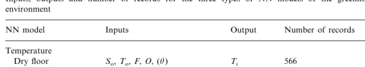
state of floor). The final list of inputs, outputs, and number of records is presented in Table 1. The reason for placinguandH in parentheses will become apparent in the next section.

3.1. Temperature models

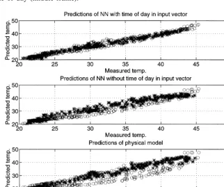
The training results of the dry-floor model are presented in Table 2. The model including the time of day in the input vector produced a high correlation between the predicted and measured temperature (R2_{=0.97). The root-mean-square (RMS)}

of the training error was 1.14 K. When the time of day was removed from the

Table 1

Inputs, outputs and number of records for the three types of NN models of the greenhouse environment

NN model Inputs Output Number of records

Temperature

So,To,F,O, (u)

Dry floor Ti 566

Wet floor So,To,F,O, (u), (H) Ti 898

CO2concentration F,O,R Xi 622

Table 2

Dry floor temperature model

Column number: 1 2

4 5

Number of input nodes

4 4

Number of hidden nodes

0.97 0.94

R2_training

RMS training (K) 1.14 1.74

0.92

R2_{test 0.97}

RMS test (K) 1.20 1.79

Neural network training results. Column 2 corresponds to the model trained without the time of day in the input vector.

input, the correlation coefficient decreased to R2_{=0.94, and the error increased to}

RMS=1.74 K. This was a significant loss of accuracy, which shows that the heat capacity of the greenhouse with a dry floor should not be ignored. The effect of the heat capacity of the greenhouse can be appreciated also in Fig. 1, which presents the predictions of the dry floor NN with the time of day (top frame), without the time of day (middle frame).

Table 3

Wet floor temperature model

Column number: 1 2 3

6

5 4

Number of input nodes

4 5 4

Number of hidden nodes

0.97 0.97

0.97 R2_training

1.20

RMS training (K)] 1.13 1.17

0.97 0.96

R2_{test 0.97}

1.16 1.21 1.24

RMS test (K)

Neural network training results. Column 2 corresponds to the model without the time of day in the input vector, and column 3 corresponds to the model with both time and relative humidity in the input vector.

In order to quantify the superiority of the NN model over a simple physical model, the following model was fitted to the data:

Ti=To+L/(rcQ+U)So (8)

Here L denotes the solar radiation heating efficiency, Q is the ventilation rate, and U is the overall heat transfer coefficient of the cover. The solar radiation heating efficiency (L) was determined using data with maximum ventilation rate, so that the heat transfer through the cover (characterized byU) could be neglected. In a second stage, the overall heat transfer coefficient of the cover (U) was determined using data with very low ventilation rate. This identification led to L=0.3 and

U=12 W/(m2_{K), with a RMS of 3.0 K. The predictions of this physical model are}

presented in the bottom frame of Fig. 1. Comparison between the middle and bottom frames shows that, with the same independent variables (inputs), the NN model gives far better predictions than the physical model.

The training results of the wet-floor greenhouse are presented in Table 3. The inclusion of the time of day had a smaller effect than in the case of the dry-floor greenhouse, as one might expect from the moderating effect of evaporation. Removing the relative humidity from the input vector only marginally affected the NN performance.

In addition to weather and control variables, the input vector of the models used in the remainder of this paper (column 1 in Tables 1 and 2) contains the time of day, which makes it difficult to present the results graphically. However, since the training data were collected on bright summer days and a strong dependence of solar radiation on the time of day was evident, the time of day in the input could be calculated from the solar radiation using the following relation, symmetrical around noon:

u=43200

p arcsin

So−100

950

u=43200

p arccos

S_o−100

Here, u is the hour of day (in seconds), and So is the outside solar radiation.

The behavior of the dry-floor and wet-floor temperature models is shown in Figs. 2 and 3, respectively. As expected, the temperature decreases with increasing ventilation, while it increases with solar radiation. An increase of outside tempera-ture also leads to an increase of temperatempera-ture (not shown here). The effect of wetting the floor is very significant. For instance, in an non-ventilated greenhouse, wetting the floor results in a temperature reduction of 6 K.

3.2. CO2 concentration model

The training results of the CO2 concentration model are presented in Table 4.

The fit, in terms of R2_{, is considerably less than the fit of the temperature model}

(R2 _{of 0.87 compared to 0.97). The RMS error, however, is only about twice as}

large as the estimated instrument error.

The behavior of the model is shown in Fig. 4. As expected, the CO₂ concentra-tion decreases asymptotically with increasing fan speed and screen opening, the asymptotic value being the outside CO₂ concentration (350 ppm). When no enrichment is used (top-left panel), the result should be an horizontal line at 350 ppm, and deviations from the expected line are a visual measure of the accuracy of the model.

Fig. 3. Predicted temperature in wet floor greenhouse.Frepresents the fan speeds,Sois the outside solar radiation,Tois the outside temperature andTiis the predicted temperature in the greenhouse.The time of the day was computed from the solar radiation according to Eqs. (9) and (10). The solid lines correspond to morning predictions, the dashed lines correspond to afternoon predictions. In each case the upper line is for a closed screen, the lower one for a fully open screen.

Note that in the case of a greenhouse occupied by a well developed crop, the CO₂ model would require at least one additional input (So), which would strongly affect

the sink for CO2, and the curves of Fig. 4 would be lower than in the present case.

4. Optimization

4.1. Statement of the problem

Using the NN models presented in the previous section, the instantaneous criterion (Eq. (3)) may be expressed as a function of the control variables F, Oand R:

Table 4 CO2model

Number of input nodes 3

4 Number of hidden nodes

R2_{training 0.87}

RMS training (ppm) 156

R2_{test 0.86}

RMS test (ppm) 163

Fig. 4. Predicted CO2concentration.Frepresents the fan speeds,Ris the enrichment rate, andXiis the predicted CO2concentration. In each graph, the upper line is for closed screen, the lower one for fully open screen, and intermediate ones correspond to 10% increments.

j=k_gg{F,O,R}−k_cR−k_eE{F} (11)

A systematic search over the three dimensional control space (F, O, R) should be able to locate the optimal control combination which maximizes j. The search was constrained by the capacity of the equipment, and by an upper limit on the allowed temperature (35°C). The optimization algorithm consisted of a simple comprehensive search over a rectangular grid, the criterion being computed in 8000 points.

4.2. Nominal solutions

Once the system sub-models were available, and the criterion j was specified, a quasi-steady-state optimization could be performed. The weather of 22 July 1994 and the nominal parameter values as listed in Appendix B were selected to represent the nominal case.

1. From sunrise until approximately 07:45 h, the enrichment gradually increases, while ventilation is rather limited. During this period, the criterion rises sharply as a result of the increase in photosynthesis, while only limited enrichment is required. 2. Between 07:45 and 12:00 h, the greenhouse has to be ventilated in order to prevent extreme greenhouse temperature (limited to 35°C). It can be seen that when the ventilation is turned on, the enrichment does not cease, but rather attains its upper limit (20 mg[CO2]/(m2s)). Since the enrichment rate is constant and the

ventilation increases, the CO2 concentration in the greenhouse decreases, which

causes the criterion to decrease.

3. At 12:00 h, the ventilation has to be increased further, which makes enrich-ment wasteful. Enrichenrich-ment is then stopped, and the fans are operated at their full capacities. In the late afternoon, since the temperature is low, the ventilation can be reduced, and enrichment can be reapplied for a short period of time.

Table 5

Daily criterion for sample day (10−3_$

/m2_d) CO2price

High Low

252 229

Dry floor

Wet floor 305 257

High CO2price is 0.44 $/kg[CO2].

Generally speaking, the present result is similar to the result obtained by Ioslovich et al. (1995), for the same crop model, an imaginary model of a dry floor greenhouse and an artificial weather sequence. The main difference is that the second phase of the present solution (relatively high ventilation rate in conjunction with maximum enrichment rate) is not present in Ioslovich’s solution, which jumps directly from our first phase to the third. There seem to be two reasons for this difference. (1) The cover-to-floor area-ratio (3.0), and hence the heat transfer through the cover, were exceptionally high in our small experimental greenhouse. (2) The upper bound on greenhouse temperature (35°C), which was not imposed in Ioslovich’s study, triggered an early transition to the second phase, which otherwise may not have occurred.

The optimal solution obtained for the wet floor greenhouse under the same weather (not shown here) reflects the positive effect of evaporative cooling. The ventilation requirement is reduced considerably, resulting in a much more efficient enrichment, and a higher daily optimal criterion (Table 5).

4.3. Results in weather space

The quasi-steady-state solution (such as Fig. 5) is a sequence of independent optimizations, which are a function of the weather variables So and To, and the

time of day u. In order to present the results in theSo−Toplane, the time of the

day was substituted by a function of So (Eqs. (9) and (10)), and the results are

presented separately for morning and afternoon hours.

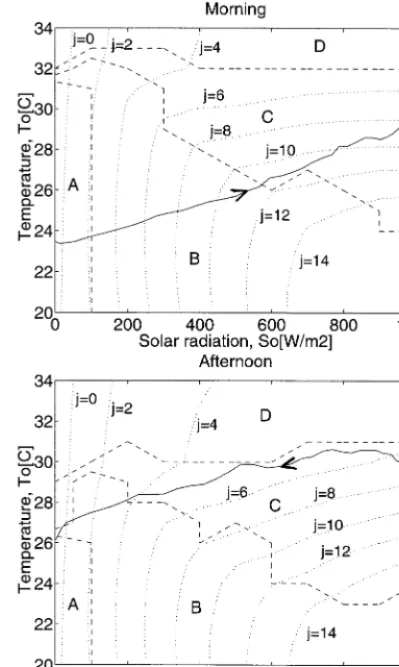
The instantaneous performance criterion, j, is shown on the same figures. As expected, the highest gain is for high solar radiation and low temperatures. As long as ventilation is not required, the criterion increases almost linearly with solar radiation, and depends very little on the outside temperature. During simultaneous ventilation and enrichment, the criterion is much more dependent on the outside temperature. At very high energy loads, when only strong ventilation is applied, the criterion depends again on the solar radiation only. Comparison between morning and afternoon, and between Figs. 6 and 7 shows that the criterion at low heat loads (Regions A and B) is rather insensitive to the time of day and the status of the floor. The latter influences mainly when switching to Region C occurs. This

Fig. 6. Optimal operating regimes and criterion values (j) (10−6_$

Fig. 7. Optimal operating regimes and criterion values (j) (10−6_$

/(m2_{s)) for wet floor greenhouse with} values for all parameters. The upper graph corresponds to morning hours, the lower one to afternoon hours. Soand Toare the outside solar radiation and temperature, respectively. A: no ventilation – no enrichment. B: enrichment without ventilation. C: simultaneous ventilation and enrichment. D: ventila-tion without enrichment.

switching also coincides with the bending of the iso-criterion curves. As a result of the heat capacity of the greenhouse, which is represented by the time of day, the onset of ventilation and the stopping of enrichment occur at lower heat loads in the afternoon than in the morning.

4.4. Effect of price of CO2

As is clear from the expression of the criterion (Eq. (11)), the location of the optimum depends on the price ratio kc/kg More expensive CO2 gas will move the

is convex upward, the second term is linear, and the third term is an order of magnitude smaller than the other two.

Fig. 8 shows the optimal operating regimes and criterion values for the dry floor greenhouse, when the price ratiokc/kgis twice the nominal one. A comparison with

Fig. 6 shows the now lower position of the border between Regions C and D. In other words, the onset of ventilation is barely affected by doubling the price ratio, but the region corresponding to simultaneous ventilation and enrichment becomes much less attractive, and switching to ventilation alone occurs at much lower energy-loads.

When the floor is wet, doubling the CO2 price has qualitatively the same effect

(Table 5), namely lowering the border between Regions C and D while leaving the border between Regions B and C roughly unchanged (not shown here).

Fig. 8. Optimal operating regimes and criterion values (j) (10−6_$

5. Conclusion

A demonstration has been given of greenhouse climate optimization based on neural network models of the greenhouse environment. The development of the NN models did not require elaborate measurements of the ventilation rate, as would be needed for the development of physical models. Only relatively easy-to-measure environmental variables and actuator positions had to be monitored. In particular, heat storage could be introduced in the model through the variable ’time of day’. By comparison, including heat storage in a physical model would require the use of an additional variable (for instance, the soil temperature), or alternatively, a dynamic model should be considered. The price of this convenience is the need for a large data set, which, presumably, could be accumulated over time in a computer-controlled greenhouse.

Although in principle a MIMO NN model could have sufficed to model both temperature and CO2 concentration with dry and wet floor, such a model

per-formed poorly when included in the optimization procedure. It became apparent that the dimensionality of the NN models should be reduced to the minimum, in order to avoid regions with sparse data. This was done by eliminating some of the potential input variables, based on a physical understanding of the system, which can be viewed as including prior knowledge in the model. Note, however, that although the loss of fit due to this simplification was minimal, the current models are limited to a narrow range of wind and humidity conditions, since they were based on summertime measurements. Adding these two factors should be attempted only when sufficient additional data become available.

The advantage of evaporative cooling, in particular for CO2enrichment, has been

demonstrated. Maintaining the permissible 35°C in our greenhouse required consid-erably less ventilation when the floor was wet than when it was dry. This prolonged considerably the duration of CO2enrichment, and resulted in a higher daily optimal

criterion (Table 5).

Acknowledgements

This study was supported by BARD, Project IS-1995-91RC, by the Israel Ministry of Agriculture, Project No. 838-0375-92, and by the Technion Fund for the Promotion of Research.

Appendix A. Nomenclature

Symbols

specific heat of air at constant pressure, J/(kg[air]K)

c

E fans energy consumption, W/m2_[ground]

vector describing weather outside greenhouse, _c e

fan operating level

F

rate of dry matter accumulation, kg[CO2]/(m2[ground]s) g

H relative humidity

vector of the greenhouse environment, _c I

instantaneous performance criterion, $/(m2_[ground]s) j

kc unit price of supplied CO2, $/kg[CO2]

unit price of electricity, $/(kWh)

ke

unit price of CO2 in biomass, $/kg[crop CO2] kg

screen opening

O

cost of control, $/(m2_[ground]s) p

photosynthetic active radiation (PAR), W/m2_[ground] P

ventilation flux, m3_/(m2_[ground]s) Q

respiration rate per unit crop mass, kg[CO₂]l(kg[crop CO₂]s)

r

CO2 enrichment flux, kg[CO2]/(m2[ground]s) R

vector describing state of crop, _c s

solar radiation flux, W/m2_[ground] S

temperature, K

T

overall heat transfer coefficient through cover, W/(m2_[ground]K) U

control vector, _c u

CO2 content of crop, kg[crop CO2]/m2[ground] w

CO2 concentration, kg[CO2]/kg[air] X

Greek symbols

extinction coefficient in F, m2_[ground]/m2_[leaf] a

b temperature response curvature, K−2

leaf conductance to CO2,kg[air]/(m2[ground]s) g

o photosynthetic efficiency, kg[CO2]/J[PAR]

ratio of PAR to solar radiation

z

L solar radiation heating efficiency respiration exponent, K−1 n

air density, kg[air]/m3 r

transmissivity of greenhouse cover to solar radiation

t

time of day, s

u

1−exp (−avw)

F

v leaf area ratio, m2_{[leaf]/kg[crop CO} 2]

Notes

bold-face symbols denote vectors 1

2 _cindicates that units are different for the various elements of the vector

Subscripts

1 large fan

small fan 2

inside greenhouse I

reference r

x at maximum

Acronyms

multiple input multiple output MIMO

neural network NN

root mean square RMS

coefficient of linear correlation R2

single input single output SISO

*

Appendix B

Physical constant

z=0.5

Greenhouse parameter

t=0.7

Photosynthesis parameters

o=10−8 _kg[CO

2]/J[PAR] g=2 10−3 _kg[air]/(m2_[ground]s) b=2×10−3 _K−2

n=0.0693 K−1 t=0 4×10−6 _kg[CO

2]/(kg[crop CO2]s) Tr=25°C

Tx=30°C

Crop parameters

w=0.1 kg[crop CO₂]/(m2_[ground]) a=0.8 m2_[ground]/m2_[leaf] v=19 m2_{[leaf]/kg[crop CO}

2]

Nominal prices

kc=0.22 $/kg[CO2] k_e=0.045 $/(kWh)

k_w=15 $/kg[crop CO₂]

NN normalization values 05F531

05O5100 05R520×10−6

05T_i550 300×10−6_5X

References

Demuth, H., Beale, M., 1992. Neural Network Toolbox for Use with Matlab: Users guide. Natick, MA.

Ioslovich, I., Seginer, I., Gutman, P.O., Borshchevsky, M., 1995. Sub-optimal CO2 enrichment of greenhouses. J. Agric. Eng. Res. 60, 117 – 136.

Kok, R., Lacroix, R., Clark, G., Taillefer, E., 1994. Imitation of a procedural greenhouse model with an artificial neural network. Can. Agric. Eng. 36 (2), 117 – 126.

Linker, R., Gutman, P.O., Seginer, I., 1997. Simultaneous control of temperature and CO2 concen-tration in greenhouses. Proceedings of IFAC/ISHS 3rd Workshop on Mathematical and Control Applications in Agriculture and Horticulture, Hannover, Germany, pp. 31 – 36.

Seginer, I., Angel, A., Gal, S., Kantz, D., 1986. Optimal CO2enrichment strategy for greenhouses: a simulation study. J. Agric. Eng. Res. 34, 285 – 304.

Seginer, I., McClendon, R.W., 1992. Methods for optimal control of the greenhouse environment. Trans. ASAE 35 (4), 1299 – 1307.

Seginer, I., Sher A., 1992. Neural-nets for greenhouse climate control. Presented at the 1992 International Summer Meeting Sponsored by ASAE, Paper No 927013.

Seginer, I., Boulard, Th., Bailey, B.J., 1994. Neural network models of the greenhouse climate. J. Agric. Eng. Res. 59, 203 – 216.

Tap, R.F., van Willigenburg, L.G., van Straten, G., van Henten, E.J., 1993. Optimal control of greenhouse climate: computation of the influence of fast and slow dynamics. Proc. 12th IFAC World Congr., Sydney, Australia, 10, 321 – 324.

van Henten, E.J., 1994. Greenhouse climate management: an optimal control approach. Ph.D. Thesis, Wageningen.