Dynamic Hedging in a Volatile Market

(1)

Dynamic Hedging in a Volatile Market

Thomas F. Coleman†, Yohan Kim‡, Yuying Li†, and Arun Verma†

May 27, 1999

1. Introduction

In financial markets, errors in option hedging can arise from two sources. First, the option value is a nonlinear function of the underlying; therefore, hedging is instanta-neous and hedging with discrete rebalancing gives rise to error. Frequent rebalancing can be impractical due to transaction costs. Second, errors in specifying the model for the underlying price movement (model specification error) can lead to poor hedge per-formance. In this article, we compare the effectiveness of dynamic hedging using the constant volatility method, the implied volatility method, and the recent volatility func-tion method [3]. We provide evidence that dynamic hedging using the volatility funcfunc-tion method [3] produces smaller hedge error. We assume that there are no transaction costs, and both the risk-free interest rate r and the dividend rateq are constant.

Many studies have shown that the classical Black-Scholes constant volatility model does not adequately describe the stock price dynamics, see e.g., [13]. Implied volatility typically exhibits a dependence on both option strike and maturity, referred to as the volatility smile. Thus the constant volatility method, which assumes that the volatility is constant for all the options on the same underlying, can lead to a significant model specification error. To reduce this error in practice, the implied volatilitymethod, which uses different constant volatilities for options with different maturities and strikes, is frequently used in pricing and hedging. Although the implied volatility method yields accurate valuation of vanilla options, it does not eliminate the model specification error. A volatility function method attempts to accurately approximate the unknown local volatility function σ(s, t) from the available market option prices in the context of a 1-factor continuous model. The computed volatility function can then be used for pricing options and determining hedge factors. This type of method follows the work of Dupire [8] who shows that the local volatility function can be uniquely determined if the prices of European options of all strikes and maturities are available. Various methods have been proposed [1, 2, 3, 5, 6, 10, 11, 12, 13] to compute a local volatility function calibrating a finite set of market option data. In the volatility function method [3], the volatility function is represend as a 2-dimensional spline; this method is distinguished from the

†_{Computer Science Department and Cornell Theory Center, Cornell University, Ithaca, NY 14850.} ‡_{Center for Applied Mathematics, Cornell University, Ithaca, NY 14850.}

∗_{Research partially supported by the Applied Mathematical Sciences Research Program (KC-04-02) of}

(2)

others in its emphasis on accurate approximation of the unknown volatility function, a key component in accurate hedging.

The main idea behind the volatility function method [3] is now brieﬂy summarized. Let a general 1-factor diﬀusion process describe the underlying price movement,

dSt

St =µ(St, t)dt+σ(St, t)dBt, (1)

where Bt represents a standard Brownian motion, µ(s, t) is the drift, and σ(s, t) is a

deterministic local volatility function. The 1-factor model (1) is calibrated with a given set of option prices to approximate the local volatility functionσ(s, t) using a spline. In [3], the local volatility function is represented by a bicubic spline which is computed by solving an inverse constrained nonlinear optimization problem as follows. Let {v¯j}mj=1

denote the m given market option prices and the number of spline knotsp≤m. Given {(¯si,¯ti)}p_i=1 spline knots with corresponding local volatility values ¯σi def= σ(¯si,¯ti), an interpolating cubic splinec(s, t; ¯σ) with a ﬁxed end condition, e.g., the natural spline end condition, is uniquely deﬁned by setting c(¯si,¯ti) = ¯σi, i = 1,· · ·, p. The local volatility

values ¯σi at knots (hence the spline) are determined by calibrating the market option

prices:

min

¯

σ∈p f(¯σ)

def

= 1 2

m

j=1

[vj(c(s, t; ¯σ))−¯vj]2

subject to l≤σ¯≤u. (2)

Additional weights can be added to take account of diﬀerent accuracies of ¯vj. The value

vj(c(s, t; ¯σ)) denotes the theoretical option price with the same maturity and strike as the given option ¯vj when the local volatility σ(s, t) = c(s, t; ¯σ). The lower and upper

bounds, l, u∈ p, l < u can be used to incorporate additional information onσ. More detailed discussion on computational issues pertaining to solving (2) can be found in [3]. The synthetic European option example used in [3, 12] demonstrates that the hedge factors computed using the constant and implied volatility methods can be erroneous. In this example, it is assumed that the underlying follows a known absolute diﬀusion process,

dSt

St =µ dt+

C

StdBt, (3)

where µ is the drift, Bt is a standard Brownian motion, and C > 0 is a constant. Here the volatility is a function of the underlying but does not depend on time. When the underlying follows the absolute diﬀusion process (3), a closed-form solution for the European options exists [4]; this closed form solution can be used to compute option prices as well as hedge factors. Let the initial underlying value beS0 = 100. Assume the

(3)

80 85 90 95 100 105 110 115 120 0.35 0.4 0.45 0.5 0.55 0.6 0.65 0.7 0.75 0.8 0.85 Underlying Delta Exact Volatility Implied Constant

80 85 90 95 100 105 110 115 120

0.006 0.007 0.008 0.009 0.01 0.011 0.012 0.013 0.014 Underlying Gamma Exact Volatility Implied Constant

0 0.2 0.4 0.6 0.8 1

0.5 0.52 0.54 0.56 0.58 0.6 0.62 0.64

Time to Maturity

Delta

Exact Volatility Implied Constant

0 0.2 0.4 0.6 0.8 1

0.005 0.01 0.015 0.02 0.025 0.03 0.035

Time to Maturity

Gamma

[image:3.612.136.471.51.323.2]

Exact Volatility Implied Constant

Figure 1: The Delta and Gamma Hedge Factors of European Call Options

difference method for solving the generalized Black-Scholes partial differential equation, the volatility function method [3] described above computes a volatility function using 22 spline knots; more details can be found in [3]. It is clear that both the delta and gamma factors computed using the volatility function method [3] are significantly more accurate compared to the constant and implied volatility methods.

The focus of this article is dynamic hedging in which a hedge portfolio is rebalanced discretely. Delta and gamma hedge factors are computed at each rebalancing time to adjust positions of the instruments in the hedge portfolio. Gamma hedging takes into account the curvature in the relationship between the option price and the underlying price, and thus produces better hedge results. To perform this second order hedging, one additional traded option on the same underlying is needed to make a portfolio both gamma and delta neutral.

(4)

2. Hedging the Synthetic European Option

We consider the synthetic European option example described in §1 since the known volatility function can be used as the benchmark for comparison. Three diﬀerent rebal-ancing frequencies n are considered, n= 52 (weekly),n= 104 (biweekly), and n= 365 (daily). For the constant volatility method, the volatility parameter is ﬁxed over the entire hedge period; the constant volatility used is C/S0, where S0 is the initial

under-lying price. For the implied volatility method, an implied volatility is obtained at every rebalancing time. For the volatility function method [3], a single volatility surface is computed at the beginning of a hedge horizon in order to avoid the computing time required to reconstruct a volatility surface at each rebalancing time for each simulation; this surface is then used for the entire hedge period.

We perform dynamic hedge simulation similar to that described in [9] to illustrate the hedge eﬀectiveness. From the diﬀusion equation (3), paths of the underlying price movement are simulated using the Euler approximation.

To compare hedge eﬀectiveness, hedge error of an option needs to be quantiﬁed. Let {ti}ni=0,ti+1 =ti+δt, denote the discrete rebalancing times in the hedge horizon, [0, τ],

0 < τ ≤ T, whereT is the maturity of the option. For delta hedging, we consider the

delta hedge portfolio {V(t), S(t), B(t)}with,

Π_∆(t) =V(t) + ∆_V(t)S(t) +B(t),

where Π∆(t), V(t), S(t), and B(t) denote the dollar values of the portfolio, option,

underlying, and money market account respectively. At the beginning of the hedge horizon, Π_∆(0) = 0, B(0) = −(V(0) +S(0)∆_V(0)) where ∆_V(0) = [∂V_∂S]_t=0 is the delta hedge factor of the option V at t = 0. At each rebalancing time ti, the hedge factor ∆_V(ti) is recomputed and the money market account is adjusted:

B(ti) =erδtB(ti−1)−S(ti)(∆V(ti)−∆V(ti−1)).

Thus the portfolio is self-ﬁnanced. The delta hedge error is deﬁned as |Π∆(τ)|, the

absolute value of the portfolio Π_∆ at the end of the hedge horizon of the option. For gamma hedging, the gamma hedge portfolio {V(t), I(t), S(t), B(t)} is formed with

ΠΓ(t) =V(t) +m1(t)S(t) +m2(t)I(t) +B(t),

where Π_Γ(t) denotes the dollar value of the portfolio, I(t) is an additional instrument, which depends on the same underlying S(t), with the maturity greater than T. The numbers of holdingsm1(t) andm2(t) are chosen such that the portfolio ΠΓ is both delta

and gamma neutral, i.e.,

∆_V(t) +m1(t) +m2(t)∆I(t) = 0

Γ_V(t) +m2(t)ΓI(t) = 0.

The values ∆_V(t),Γ_V(t) are the delta and gamma factors for the optionV(t); the values ∆_I(t),Γ_I(t) are delta and gamma for the option I(t). At the beginning of the hedge horizon, ΠΓ(0) = 0,B(0) =−(V(0) +S(0)m1(0) +I(0)m2(0)). At each rebalancing time

ti, both delta and gamma hedge factors are recomputed and the money market account is adjusted:

(5)

Rebalancing Frequency n=52 n =104 n=365

Delta Hedging

Constant Volatility .1108 .1005 .0890 Implied Volatility .1188 .1112 .0969 Volatility Function .0803 .0610 .0392 Exact Volatility .0771 .0580 .0292

Gamma Hedging

[image:5.612.159.448.50.178.2]

Constant Volatility .0251 .0233 .0224 Implied Volatility .0256 .0244 .0235 Volatility Function .0138 .0134 .0121 Exact Volatility .0074 .0041 .0015

Table 1: Average Relative Hedge Errors Over 200 Sample Paths: A Synthetic Example

The gamma hedge error is deﬁned as |Π_Γ(τ)|, the absolute value of the gamma hedge portfolio ΠΓ at the end of the hedge horizon of the option.

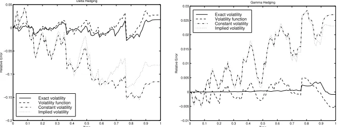
Table 1 displays the average relative hedge errors at the maturity for the synthetic European call option with the strike K = 100, maturity T = 1 and τ = T in the described dynamic hedge simulation. The average relative hedge error is deﬁned as the average of the hedge errors at the maturity over the 200 price simulation paths divided by the initial option price V(0) = $18.58. For gamma hedging, the put option with the strikeX = 98 and maturity T = 1.1 is used as the additional instrument. To illustrate the change of the hedge portfolio values in the course of the hedge period, the relative values of the hedge portfolios are graphed in Figure 2 for a sample path in one year with the rebalancing frequency n= 104.

0 0.1 0.2 0.3 0.4 0.5 0.6 0.7 0.8 0.9 1

−0.2

−0.15

−0.1

−0.05

0 0.05

Delta Hedging

Time

Relative Error

Exact volatility Volatility function Constant volatility Implied volatility

0 0.1 0.2 0.3 0.4 0.5 0.6 0.7 0.8 0.9 1

−0.01

−0.005 0 0.005 0.01 0.015 0.02 0.025 0.03

Gamma Hedging

Time

Relative Error

Exact volatility Volatility function Constant volatility Implied volatility

Figure 2: The Relative Values of the Hedge Portfolios Along a Sample Path

[image:5.612.136.470.389.515.2]

(6)

constant and implied volatility methods do not decrease as quickly when the hedge portfolios are rebalanced more often.

3. Hedging the S&P 500 Futures Options

The synthetic example in §2 demonstrates that both delta and gamma hedge errors using the volatility function method [3] are signiﬁcantly smaller than those from using the implied and constant volatility methods; the delta hedge error using the volatility function method [3] is close to that from using the true volatility function. However, this encouraging performance on synthetic data does not immediately imply that hedging with the volatility function method [3] is better in a real market. Calibrating from the market option prices and following the market price movement, we now provide evidence illustrating the advantages of using the volatility function method [3] in dynamic hedging. We consider dynamic hedging for the S&P 500 futures options traded in Chicago Mercantile Exchange. Here the market futures price movement is used as the path against which hedge performance is measured. Although these options are American, the spline inverse optimization formulation (2) remains a reasonable way to estimate the local volatility function from a given set of option prices; the American option values are computed using a partial diﬀerential equation approach as described in [9].

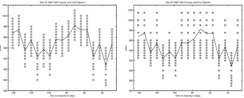
We consider the market futures option price data from May 1997 to March 1998. There are three index futures in this data set: the first index future matures on September 18, 1997, the second on December 18 1997, and the third on March 19 1998. The futures and options mature on the same day. Therefore, we correspondingly separate the option prices into three data sets. We choose, on each Wednesday, 12 calls and 12 puts whose strikes are nearest to the futures price; we only consider at-the-money and near-the-money options since their prices are more accurate than deep in-the-money or out-of-the-money options. Thus the first data set contains call and put options on the S&P 500 September 97 index futures from May 21 to September 10 in 1997. The second data set contains option prices on the December 97 futures from July 30 to November 19, 1997. The third data set includes options on the March 98 futures from January 7 to March 11, 1998. The third data set covers relatively shorter period than the first two since we do not have the option prices on the March 98 futures near the end of 1997. The hedge portfolios are rebalanced weekly; the volatility function, implied volatility, constant volatility parameter, and hedge factors are recomputed weekly. Figure 3 displays the futures prices and option strikes in the first data set for the September 18, 1997 futures; the solid line depicts the futures prices and the circles/squares display the strikes of the call/put options.

For the constant volatility method, we choose the constant which best fits for the 12 call option prices in the least squares sense. The volatility parameter for the put options is defined similarly. In the implied volatility method, each option has a different implied volatility parameter. For the volatility function method [3], a volatility surface is computed, at each rebalancing time, by solving (2) using the 24 call and put options with 9 spline knots placed on the mesh,

[.6S0, S0,1.4S0]T ×[0, .25T, .75T],

where S0 denotes the initial futures price andT is the maturity. We perform one week

(7)

40 60 80 100 120 140 860 880 900 920 940 960 980 1000 1020

Dec 97 S&P 500 Futures and Call Options

time to maturity in days

price

40 60 80 100 120 140 860 880 900 920 940 960 980 1000 1020

time to maturity in days

price

[image:7.612.105.504.51.211.2]

Dec 97 S&P 500 Futures and Put Options

Figure 3: Futures and the Option Strikes for the September 18, 1997 Data Set

gamma hedge factors of options are computed using each of the three methods; options are hedged for a 1-week period using these hedge factors.

Table 2–4 display the average weekly hedge errors and the standard deviations using the constant volatility, implied volatility, and the volatility function method [3]. The average weekly hedge error is the sum of the weekly hedge errors of all the options in the data set divided by the number of options. The numbers in the parenthesis are the standard deviations of the hedge errors.

Call Put

Delta Hedging

Constant Volatility 1.6474 (1.3170) 1.6310 (1.2966) Implied Volatility 1.6348 (1.3126) 1.6188 (1.2885) Volatility Function 1.4339 (1.2052) 1.4154 (1.1837)

Gamma Hedging

Table 2: Hedge Error : Options On The Sep 97 Futures

Call Put

Delta Hedging

Gamma Hedging

Table 3: Hedge Error : Options On The Dec 97 Futures

(8)

Call Put

Delta Hedging

Gamma Hedging

[image:8.612.141.467.53.150.2]

Table 4: Hedge Error : Options On The Mar 98 Futures

error; gamma hedging also leads to smaller errors. The most signiﬁcant performance diﬀerences between the volatility function method [3] and the constant and implied volatility methods occur in the December 97 futures data set. We note that the hedge performance of the volatility function method [3] depends on the choice for the number of knots and their placement. These decisions should in general be made by some cross validation method.

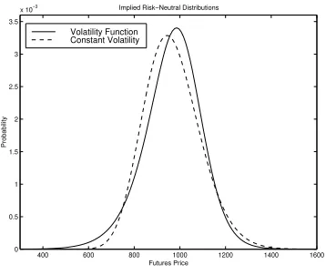
The volatility smile exhibited in an option index market indicates that the price distribution is not lognormal; indeed the implied distribution from the volatility func-tion method [3] is typically not lognormal. Figure 4 illustrates the implied risk neutral distribution of the December 97 futures as seen on August 6, 1997; the risk neutral dis-tribution of the constant volatility model is graphed for comparison. Each risk neutral distribution is computed using the Fokker-Planck equation [7].

400 600 800 1000 1200 1400 1600

0 0.5 1 1.5 2 2.5 3 3.5

x 10−3 Implied Risk−Neutral Distributions

Probability

Futures Price Volatility Function Constant Volatility

Figure 4: Comparison of the Implied Risk-Neutral Distributions

4. Concluding Remarks

[image:8.612.213.392.376.527.2]

(9)

describe the underlying price dynamics. Assuming that the price of the underlying follows a 1-factor continuous diffusion process, it is important to accurately reconstruct the local volatility function for option hedging as well as pricing. In this paper, we compare the performance of dynamic hedging using the constant volatility method, the implied volatility method, and the volatility function method [3]. With a synthetic European option example, we demonstrate that the volatility function method [3] yields significantly more accurate hedge factors and smaller hedge errors. Using the S&P 500 futures option market data and hedging against the market futures price movement, the volatility function method [3] is shown to perform significantly better in dynamic hedging when compared with the constant and implied volatility methods.

References

[1] Leif Andersen and Rupert Brotherton-Ratcliffe. The equity option volatility smile: an implicit finite-difference approach. The Journal of Computational Finance, 1(2):5–32, 1998.

[2] M. Avellaneda, C. Friedman, R. Holemes, and D. Samperi. Calibrating volatility surfaces via relative entropy minimization. Applied Mathematical Finance, 4:37–64, 1997.

[3] Thomas F. Coleman, Yuying Li, and Arun Verma. Reconstructing the unknown local volatility function. The Journal of Computational Finance, 2(3):77–102, 1999.

[4] J. C. Cox and S. A. Ross. The valuation of options for alternative stochastic pro-cesses. Journal of Financial Economics, 3:145–166, 1976.

[5] E Derman and I Kani. Riding on a smile. Risk, 7:32–39, 1994.

[6] E Derman and I Kani. The local volatility surface: Unlocking the information in index option prices. Financial Analysts Journal, pages 25–36, 1996.

[7] Darrell Duﬃe. Dynamic Asset Pricing Theory. Princeton, 1996.

[8] B. Dupire. Pricing with a smile. Risk, 7:18–20, 1994.

[9] J. Hull. Options, Futures, and Other Derivatives. Prentice Hull, 1997.

[10] N. Jackson, E. S¨uli, and S. Howison. Computation of deterministic volatility sur-faces. The Journal of Computational Finance, 2(2):5–32, 1999.

[11] Jens Jackwerth and Mark Rubinstein. Recovering probability distributions from option prices. The Journal of Finance, 51(5):1611–1631, 1996.

[12] R. Lagnado and S. Osher. Reconciling diﬀerences. Risk, 10:79–83, 1997.