The random-time binomial model

23 (1999) 1355}1386

The random-time binomial model

Dietmar P.J. Leisen*

Stanford University, Hoover Institution, Stanford, CA 94305, USA

Abstract

In this paper we study a binomial model with random time steps and explain how to calculate values for European and American call and put options. We prove both weak convergence of the discrete processes to the Black}Scholes setup and convergence of the values for European and American put options. Computational experiments exhibit a smooth convergence structure and suggest that we can obtain a quadratic order of convergence via an extrapolation procedure. Approximations to jump-di!usions are straightforward. 1999 Elsevier Science B.V. All rights reserved.

JEL classixcation: C63; G13

Keywords: Binomial model; Option valuation; Lattice approach

1. Introduction

In a continuous setup where the evolution of a single stock is modelled by geometric Brownian motion, Black and Scholes (1973) derived a closed-form solution for the value of European-style call and put options by presenting

a strategy that duplicates its payo!through continuous trading in the stock and

the bond. Later Harrison and Kreps (1979) and Harrison and Pliska (1981) developed the equivalent martingale measure concept, which gives an elegant

*E-mail: [email protected].

This paper is one of the winning entries of the graduate student paper prize awarded by the Society of Computational Economics.

technique to express and solve pricing problems in terms of expected discounted

payo!s.

This paper addresses the pricing of American put options in the Black}

Scholes setup. No closed-form solution is known to this problem, and prices

need to be calculated numerically. The main"nancial tools for this purpose are

binomial models, partial di!erential equations and the Monte-Carlo technique.

Other approaches have been adopted from the literature on numerical dynamic programming, e.g., Carr and Faguet (1996) and Meyer and Van der Hoek (1997)

using Rothe's method of lines.

Cox et al. (1979) (henceforth CRR) and Rendleman and Bartter (1979) inde-pendently presented the binomial model, which is a discrete process

approxima-tion of the original Black}Scholes framework. Binomial models are an easy

way to explain continuous trading and in"nite spanning. Furthermore,

bi-nomial models can yield simple approximations for option values where no closed-form solution is available as, for example, for the American put option. Binomial models were generalized by He (1990) to a basket of lognormally

distributed assets and Nelson and Ramaswamy (1990) to general di!usion

processes.

Monte-Carlo methods were introduced as a "nance pricing tool by Boyle

(1976). They rely on the equivalent martingale measure technique which

calcu-lates prices as expected discounted payo!s. After discretizing the time axis by

a re"nementn, a sequence ofmprice path trajectories is simulated according to

the risk-neutral dynamics and the corresponding mean and variance of the

payo! is calculated. According to the Law of Large Numbers the empirical

mean converges to the true price for European-style options. The empirical variance gives an estimation of how close the mean is to the correct price in

a model with re"nementnof the time axis. A great advantage of the

Monte-Carlo approach is its being readily applicable to any pricing problem. For an overview on the state-of-the-art of Monte-Carlo techniques in option pricing, see Boyle et al. (1997).

Monte-Carlo techniques are suggested as a solution to the&curse of

dimen-sionality'. In binomial models with a"xed re"nement the computational cost

exponentially increases by the number of assets, but it is independent for Monte-Carlo techniques. For American put options the exercise decision and the price are upward biased; the downward biased estimator constructed re-cently by Broadie and Glasserman (1997) now allows valuing these options

properly, too. Their approach is closely related to the&random multigrid'of Rust

(1997) for solving dynamic programming problems. Rust (1997) analyzed the

There also exists a di!erent interpretation for binomial models: Black and Scholes (1973) noted

that"nancial derivatives must ful"l a speci"c partial di!erential equation. Discretizing this by

complexity of his approach and proved that it is successful in breaking the&curse

of dimensionality'for discrete decision processes.

This paper focuses on the one-dimensional Black}Scholes setup where the

&curse of dimensionality' does not apply. Improvements of the original CRR

approach have been suggested by several authors: Jarrow and Rudd (1983), Boyle (1988) and Tian (1993). Leisen and Reimer (1996) proved that the order of convergence in pricing European options for these variations is equal to one, which is also the order of convergence of CRR; thus, the many improvements on the CRR model are all equivalent. Furthermore, the convergence structure

exhibits waves and is not monotonic. This is unsatisfactory since e!ective use of

extrapolation would require a convergence structure as smooth as possible. Whereas this problem can be addressed in the case of European put options, no adjustments are known for the early-exercise premium of American put options.

The idea of approximating the Black}Scholes setup by a binomial model with

random time steps appeared in FoKllmer and Sondermann (1986) and

Sonder-mann (1987) in the form of a two-sided compound jump process. Binomial models with random time steps recently have been reconsidered by Dengler and Jarrow (1997) and Rogers and Stapleton (1998). The latter studied a model in the

Black}Scholes framework where the hedging portfolio is adjusted when certain

prespeci"ed barrier lines are reached. Although this is a clever way to value

barrier options, it faces the drawback that the distribution of the number of jumps needs to be approximated.

Our random-time binomial model assumes that the di!erence between two

trading dates is random. The main contribution of this paper is that such a randomized model smoothes the convergence structure and results in quad-ratic convergence order by extrapolation. We do not present a formal proof.

However, this is suggested by simulations and a detailed analysis of the de"

-ciencies of previous models. It makes our approach a competitive valuation tool. We suppose that a Poisson process is driving the jumps, i.e., the time increment is exponentially distributed. We also present an easy valuation formula for European style options. In a further step we extend it to the valuation of American put options. Related to our approach is Carr (1997), who uses exponentially distributed random variables to study contracts with random maturity.

A second contribution is that our model can be used in a natural way to

construct approximations for jump di!usions. Such a model has been suggested

as a response to the observation that market participants are well aware of

sudden strong price changes (&crashes'). In fact, the assumption of continuous

sample paths has also been criticized in empirical studies (see, for example, Jarrow and Rosenfeld, 1984; Ball and Torous, 1985; Jorion, 1988). Here, we adopt the framework of Merton (1976) who superimposed a compound Poisson

process on the Black}Scholes setup. Whereas geometric Brownian motion

describes the arrival of &normal' information, the jump part models large

A discrete framework for the valuation of options in this setup was given by Amin (1993). The jump part was simply put on top of the binomial model. In contrast it is merely an adjustment to the intensity of the driving process in our model. The remainder of the paper is organized as follows. In Section 2 we review the

Black}Scholes setup and the binomial model. Section 3 discusses numerical

issues related to the structure of convergence. Section 4 presents our model and

necessary and su$cient conditions for weak convergence to geometric

Brownian motion. Section 5 discusses the valuation of European and American

options. Section 6 discusses jump di!usions. Section 7 concludes the paper.

Throughout the paper, all"gures related to practical implementations use the

same parameter selection of a put option with strike 110 and one year maturity,

written on a stock with today's price equal to 100 and whose volatility is 0.3

when the short-term interest rate is equal to 0.1. All proofs are postponed to the appendix.

2. Binomial models

We suppose that the stock price process can be described under the objective measure, as in Black and Scholes (1973), by

S R"S

exp+kt#p=

R,, (1)

where thedriftkand the interest rater, as well as thevolatilityp, are supposed to

be constant. (=

R)Ris a standard Wiener process on a suitable probability space

(X,F,Q). It can be seen that E[S

R]"S

exp+kt#(p/2)t, for all t50. We

assume thatk"r!p/2 under the measure Q, which is then the risk-neutral

measure. According to Harrison and Pliska (1981), option prices are

expecta-tions w.r.t.Q.

A European call option gives its holder the right to buy the stock at some date

¹for a priceK. If the holder rationally decides to exercise the option}i.e. if

S₂5K } by selling the stock immediately thereafter, he incurs a pro"t of

S

2!K. The payo! is therefore determined by the function f:xC(x!K)>.

Similarly, a European put option gives the owner the right to sell and is

described byf:x_C(K!x)>. Black and Scholes (1973) were the"rst to present

price formulae for these options:

C(S,¹,K,p,r)"SN(d

)!Ke\P2N(d

) for a call, (2)

P(S,¹,K,p,r)"Ke\P2N(!d

)!SN(!d

) for a put, (3)

where d

"ln(S/K)

#(r$p)¹

p(¹

An American option gives its holder the right to exercise the claim at any date

up to maturity¹. Merton (1973) pointed out that an American call option on

a dividend-free stock should never be exercised prior to maturity, and so the price is equal to its European counterpart. This is no longer true for an American put option, whose price is

P"sup

NZS

E[e\PN(K!S

N)>], (4)

whereSdenotes the set of stopping times (&policies') smaller than maturity¹,

adapted to the"ltration generated by the stock process (S

R)R(see Myneni, 1992).

No closed-form solution is known forP.

For an American put option with maturity date ¹, we know from Van

Moerbeke (1976) that there is a smooth functiont_CB

Rseparating the time-state

space into two regions: the option should be exercised if}and only if}the stock

price at time t is below or at B

R. From Carr et al. (1992), we know that the

so-called early-exercise premiumn"P!Ptakes the form

n"rK

e\PRE[I

R] dt. (5)

Here, for any t3[0,¹],I

R denotes the cash-or-nothing option with strike

B_Rand maturity datet, i.e., the option paying one unit attif the stock price at

that date is below or equal toB_Rand zero, otherwise.

In the following it will be more convenient to work on the logarithmic stock

price process, since it is homoscedastic. Let us de"ne

X R"ln(S

R/S) 0 XR"kt#p=

R. (6)

Now take two sequences (i

L)LZ-, (v_L)_LZ-L1, with i

L"_O(1/n). For any re_"

ne-mentn, a discrete setup is de"ned by the setTL"+0"t L(t

L2(t

LL"¹,

of equidistant trading datest

LG>!t

LG"*t

L"¹/n.

The per period return in the risk-less bond is r

L"exp+r*t

L,; and the per

period return in the asset is modeled by the sequence of (RM

LG)Gof i.i.d. random

variables

RM

LG&

L, qL, i_L!v

L, 1!q

L,

(7)

whereq

Lwill be speci"ed later. Denote for all 04t4¹:

XM L R ",

L

R

G

and

S_ML R "S

expXM RL,

where

NL

R " .

The process (S_ML

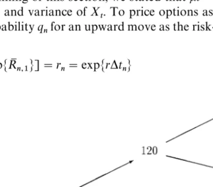
R )XRX2is called abinomial modelwith re"nementn. An example

for possible dynamics is given in Fig. 1, where we assume a re"nement ofn"2,

today's stock priceS

"100, andi

L#v

L"ln 1.2,i

L!v

L"ln 0.9.

We denote byN the weak convergence (also called convergence in

distribu-tion) for stochastic processes. A necessary condition forXM LN Xis the

conver-gence of any"nite-dimensional distribution at datet. This requires

E

*t_L

and

Var(R_M L)

*t L

L

Pp. (9)

At the beginning of this section, we stated thatkt"(r!p/2)tandptare the

expectation and variance ofX

R. To price options as expected payo!s, we must

set the probabilityq

Lfor an upward move as the risk-neutral probability, i.e., for

givenv

L,iL

E[exp+RM

L,]"r

L"exp+r*t

L, (10)

must hold. In the series expansion of the exponential function, it can be

checked that, if condition (8) is ful"lled, the martingale measure

condi-tion E[exp+R_M

L,]"exp+r*t

L, is matched up to second-order terms. For the

logarithmic process X, condition (8) corresponds to Eq. (10). We therefore

require the equality E[RM

L]"k*t

L. It is straightforward to show that

q_L"k*tL !i

L#v

L

2v L

.

Using Eq. (8) and the equality Var(RM

K)"E[(RM

K)]!E[RM

K]"v

L!

E[RM_K], we see that condition (9) requires

"v_L" (*t

L L

Pp.

To ful"l this condition,v

Lis chosen equal top(*tL. The models proposed in the

literature di!er in the speci"cation ofi

L:

(1) Jarrow and Rudd (1983):

Setting∀n:i_L": (r!p/2)*t

L, we getqL".

(2) Cox et al. (1979):

Setting∀n:i_L": 0, we getq

L"#[(r!p/2)/2p](*t

L.

We call the vector (u

L,dL,rL,qL)"(exp(i

L#v

L), exp(iL!v

L), exp+r*tL,,qL) the

characteristic terms of the speci"c binomial model under consideration.

Al-thoughr

LandqLare somewhat redundant, we prefer to include both since this

will make the exposition in Section 5 easier. We can now state a general convergence

Theorem 1. For a sequence of binomial models which fulxl conditions(8)and(9),we

have

XM LN X

and

SMLN S.

Using Theorem 1 we deduce that SLN S for the models proposed in the

literature. Since the payo!function for the European put is bounded,

The remainder of this section treats pricing in a "xed binomial model with

characteristic terms (u

L,dL,rL,qL). IfS is the current stock price at datetLG, the

European option price can be calculated as discounted expected prices at the

next trading datet

LG>:

P_L(t_LG,S)"r\

L E[PL(tLG>,SexpRLG)]

"r\

L +qLPL(tLG>,SuL)#(1!q

L)PL(tLG>,SdL),.

Since the conditional terminal payo! is known, backward induction yields

today's option price.

The algorithm is slightly modi"ed for an American option. We check at each

point in time whether exercise might yield a higher payo!, taking the maximum

with (K!S)>, i.e.,

P_L(t_LG,S)"max+(K!S)>,r\

L E[PL(tLG>,SexpRLG)],.

At each time t

LG, BGL will denote the highest node at which exercise occurs.

A backward induction argument performed in Leisen (1998) is used to deduce

a description for the discrete early-exercise premiumn

L"P

L!P

L in terms of

the discrete boundaryBL"(BL

G )G: n_L"n

L#n

L, (11)

where

n_L"L\

G

r\_LGK(1!r\

L )E[I L_RLG] (12)

and

n_L"L\

G

r\G

L E[1_1GL_{X G}L_{_SL1G}L _G>L(f(u_LS_GL)!r\_L P_L(tLG>,u_LS_GL))]. (13)

Here, 1denotes the indicator random variable corresponding to the setAand

I _L

RLGis de"ned similarly to the continuous case.

3. The convergence structure in binomial models

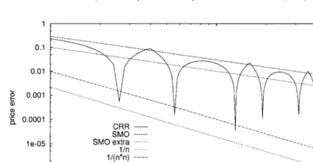
Fig. 2. Error picture for the European put option.

3.1. The European put option

Fig. 2 shows the errore

L""P!P

L" in calculating European put prices for

the parametersS

"100,K"110,¹"1,r"0.1,p"0.3. This selection will

be used in"gures throughout this paper in order to make them comparable. In

all "gures the resulting errors for the di!erent re"nements are connected by

straight lines to present the convergence structure more clearly.

In Fig. 2 we iterated over even re"nementsn"10, 12,2, 1000. For the CRR

model we observe quite erratic convergence to the continuous time solution

with waves. Iterating over all integersn"10,₂, 1000 would result in a"gure

where the waves are even more pronounced. Fairly high re"nements are

re-quired to achieve su$ciently high accuracy. In Fig. 2, e.g., at least, a re"nement

of n"200 is necessary to ensure&penny-accuracy'. We did not depict a price

picture because the error is of most interest. Furthermore, it would exhibit even worse behaviour since price approximations that overestimate the continuous time price are followed by others that underestimate. We have chosen

a log}log-scale; exponential functionsxCc/nM(c,o31>) become straight lines

which intersect logcatn"1 and slope!o. Looking at the functionnC1/n,

the "gure suggests that the order of convergence is one. Indeed Leisen and

Reimer (1996) proved this result.

The oscillations in Fig. 2 are due to the fact that the payo! function of the

European put is not di!erentiable at the strike price. At maturity the di!erence

between two adjacent nodes isu_L!d

L"O(v

L)"O(p(*t

L), and the probability

of a single node at the centre of the tree is of orderO((*t_L) (see Feller, 1966). So,

rounding o!the strike to the next node induces distortions of order O(*t

L) in

Leisen and Reimer, 1996). To remove these waves, the position of the grid in

relation to the strike needs to be controlled: the strikeK should always lie at

a"xed proportional distance to the next two grid nodes, independent of the

re"nement; e.g., the strike should be on a node. Leisen (1998) presented the

following model for even re"nementsn:

i_L"lnK/S

n and vL"p(*tL.

It changes the drift in such a way that the centre grid point of the tree lies"xed

onK for any even re"nement. This model yields a very smooth convergence

structure. It was therefore called SMO (&smooth') (see Fig. 2). The results of

Leisen and Reimer (1996) can be used to prove that the order is one.

3.2. Extrapolation

Since European put option prices typically converge with order one, their

errore

Lcan be represented by

a(n)

n #

a(n)

n

for suitable real valued functions a

()) anda

()) with a

bounded. For two

re"nements n

and n with n'n

and corresponding prices PL,PL, let us

suppose for a moment that the functiona()) is constant, equal toa

, and that

the function a,0. That is, P

L"a

/n#P

LL, where PLL denotes the

approximation forPunder this assumption. We then resolve

P L"

a n

#P

LL, (14)

P L"

a n

#P

LL, (15)

N P

LL" nP_L

!nPL n

!n

. (16)

Eq. (16) is called theextrapolation rule. We denote bye_L

Lthe errorPLL!P

resulting from extrapolation. Further analysis reveals

e

LL" a(n

)!a

(n)

n

!n

#na(n) !n

a(n)

n

n(n!n

)

. (17)

Let us set a"max

La(n)!min

La(n). If a()) is not constant, we have

e

interpreted as a measure of smoothness or as a measure for possible

improve-ments by extrapolation. The important case is the one of a constanta

. Then the

"rst term on the right-hand side of Eq. (17) vanishes. Iterating the re"nement

n and using the sequence (n, 2n) for extrapolation, Eq. (17) becomes

e

LL"(a

(2n)!a

(n))/n. So for a bounded, extrapolated prices converge

with order two. For models with constanta

, the error picture looks&smooth'.

We try, therefore, to construct new models with this property; this is why we loosely speak of smoothing options when constructing better performing models (see Leisen, 1998 for a detailed discussion).

Fig. 2 shows the errore

LLresulting from extrapolating SMO while iterating

n"10, 12,₂, 1000. A comparison with the 1/nline suggests that order two in

nholds. This con"rms our preceding analysis. We would like to point out that

this improvement holds for any parameter selection, although we depicted only one example.

3.3. The early-exercise premium

This subsection studies the additional price component in American put options resulting from the possibility of exercising them before maturity. This is

given by the early-exercise premian"P!P (see Eq. (5)) andn

L"P

L!P

L

(see Eqs. (11)}(13)). We present the numerical problems and explain our

ap-proach to improve them. Only the errors resulting from the "rst component

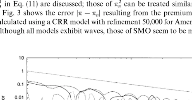
n_L in Eq. (11) are discussed; those ofn

L can be treated similarly.

Fig. 3 shows the error"n!n

L"resulting from the premium. True prices are

calculated using a CRR model with re"nement 50,000 for American put options.

Although all models exhibit waves, those of SMO seem to be more regular than

those of CRR. Since the order appears to be one, we applied the extrapolation

rule (16) iterating the re"nementnand using the sequence (n, 2n) as in Section

3.1. Extrapolating SMO no longer gives signi"cant improvements. SMO yields

better results for options where the premium is small in comparison to the European put component, i.e., those where the boundary is quite far from

today's stock price. Our speci"c parameter selection is not only of theoretical

interest, but illustrates the remaining numerical problems as well as representing the typical one in applications.

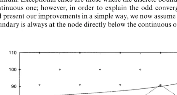
Fig. 4 exhibits the&continuous-time'boundary, calculated in a CRR model

with a re"nement of 100,000, to explain the reason, why the convergence

behaviour of the premium has worsened. The points represent the discrete stock

grid of a CRR model with re"nement n"10. We connected the discrete

boundary points (t,B ),2, (t,B ) by straight lines; they represent an

approximation to the continuous boundary. The discrete boundary seems to move in a zig-zag pattern up and down one layer of nodes. Although there are some exceptions, generally the boundary is at the node immediately below the continuous boundary. When the distance becomes too large; it jumps an entire layer following the upward trend in the continuous boundary. Near maturity

where the slope of the continuous boundary becomes in"nity, the jumps become

more and more frequent.

The boundary behaviour has an impact on the approximation structure of the premium. Exceptional cases are those where the discrete boundary is above the continuous one; however, in order to explain the odd convergence behaviour and present our improvements in a simple way, we now assume that the discrete boundary is always at the node directly below the continuous one. Then we can

treat BL as the &e!ective' cut-o! of B to the node immediately below, i.e., I L

RLIin Eq. (12) can be treated asI RLI. ComparingnLwith the representation of

the continuous boundary in Eq. (5), we note "rst that exp+!rt

LI,"r\I

L .

Approximating 1!r\

L "1!exp+!r*t

L,"r*t

L#_O(*t

L), the summation

can be treated essentially as a trapezoidal approximation to the integral; in both

cases expectations are taken over indicator functions of typeI

R. At each date,

the cut-o! problem is the same as in the European put option case: with

changing re"nement, the di!erence between the boundary and the next grid

point below will change. SMO placed nodes only at the critical point}the strike

}at terminal time and not on the boundary at intermediate time. This explains

why the convergence behaviour is no longer smooth.

Unfortunately, as the functional form of the early-exercise boundary is un-known, it is not feasible to place nodes on it. We address the problem here from

an entirely di!erent perspective and try to smooth variations in the overall

distance between the discrete and the continuous boundary over time when

changing re"nement. Heuristically, this is a way to minimize changes in the

di!erence between the discrete and the continuous boundary at a"xed time for

changing re"nements. To do so, take two models with di!erent re"nements but

the same up and down factors u,d, where the boundary does not evolve in

a completely synchronous way. If the discrete boundary approximation is

a round-o!of the continuous one to the next node below, this is the&standard'

case (remember the zig-zag structure). A "ctitious mean boundary can be

calculated by averaging with equal weight one half the (linearly interpolated) boundaries resulting from both models. In those situations where both bound-aries are moving up or down, there will be no change, however in those situations where they move in an asynchronous way, the new approximation

will be #at. Consequently, the boundary will exhibit less variation, i.e., it will

appear to be smoother.

An extension of this idea is necessary. If we reinterpret the weights as

probabilities, we can think of this approach as a mix of di!erent binomial

models, drawing one randomly as the true dynamics. However, mixing random-ly over two models is hardrandom-ly a realistic dynamics for the evolution of the price of

some underlying asset. At the "rst trading date, the information about the

underlying binomial model will be fully revealed. The optimal exercise decision in the future will then be based on this newly revealed information, and not on an average of the two early-exercise boundaries. But this averaging is what we are trying to achieve in some market model. Therefore, we need to formalize it

di!erently. To prevent the information about the underlying model of the actual

dynamics from being fully revealed after the"rst time step, we will randomize

the time between two trading dates, each increment being independent of the previous one. This will also resolve the second problem: we can expect a good approximation only if we mix over a whole sequence of binomial models with

4. Randomization of the Binomial model

This section extends the previous approaches, allowing the time increment between two trading dates to be random. Our discrete process is constructed

such as to ensure weak-convergence to the Black}Scholes setup. The next

section addresses the option valuation problem.

We start with two sequences (*x_K)_KZ-, (j_K)_KZ-L1 with *x

KPK 0,j

KPRK ,

and for eachm3-, a Poisson processNK"(NK

R )RYwith intensityjK.m

cor-responds to a re"nement of the state space. Let us recall that by denoting theith

interarrival time byq_KG, the processNK is described by

1. (q

KG)Gare independent exponentially random variables with parameter 1/jK,

2. NK

R "max+n" LG

qKG4t,.

For anym, take a sequence of i.i.d. random variables (R_KG)_G, where each element

is also independent ofNKand distributed according to

R_KG&

x_K, p_K,

!*x

K, 1!p

K.

(18)

Binomial models assume that the change in the processXbetween two trading

datest

LG,tLG>3TLis given by i.i.d. random variablesR

LG. Similarly, here we

will now approximate it by i.i.d. random variablesR

KGbetween two interarrival

timesq

KG,qKG>. In the sequel, we further assume that each element of (RKG)Gis

independent ofNK. We de"ne the processes

X_RK",

K

R

G

R_KG and S_RK"expXK

R

and call them therandom-time binomial model(henceforthRTBM). Then we have

the following.

Theorem 2. Necessary conditions forXKN Xare that for allt'0:

E[R

KG]jKPK k (19)

and

Var[R

KG]jKPK p. (20)

Please recall from the beginning of Section 2 that k"r!p/2. These two

Theorem 3. For the RTBM,suppose that conditions(19)and(20)are fulxlled.Then,

XKN X and SKN S.

We would like to remark that j_KP RK implies E[q

K]PK 0. This can be

interpreted in the sense that withmbeing su$ciently great, it can be expected

that jumps will almost always occur. Indeed, Theorem 3 tells us that, for suitably

adjusted return variables ( exp+R

KG,)KG, in the limit mPR geometric

Brownian motion is obtained. Condition (19) in Theorem 2 requires

E[R

KG]"j

K (21)

0 q K"1

2#

k

2j_K*x_K. (22)

Although we have taken (*x

K)Kand (jK)K as inputs, both cannot be chosen

independently of the other to ensure convergence to the Black}Scholes setup.

Similar to the standard binomial case where we deduced the asymptotic form of (v

L)L, here we deduce from condition (20):

Lemma 4. A necessary condition for convergence to the Black}Scholes setup is that

asymptotically

j_K&

*x_K

.

Allowing the time increment in the binomial model to be random introduces a further risk and the market becomes incomplete. Whereas in the original binomial model framework of the previous section there was a unique

equiva-lent martingale measure}represented byq

K}here we are losing this property.

Instead we have a whole set of equivalent martingale measures, all compatible with the assumption of absence of arbitrage opportunities. We can index them

by the jump-intensity j_K. For valuation purposes we need to choose one

measure among all. Yet, this cancels out in the limit according to Theorem 3. The easiest way to meet the asymptotic form of Lemma 4 is obtained by setting

j_K"

*x K

, (23)

which we adopt in the sequel. Under this choice, we deduce from Eq. (22) that

q K"1

2#

k

For any*x

Kand (RKG)Gas in Eq. (18), our RTBM is completely described by the

characteristic terms (u

K,dK,qK,jK)"(exp+*x

K,, exp+!*x

K,,#k/(2p)*x

K,

(p/*x K)).

Taking "ctitiously*x

K"p(*t

L, the only di!erence with the CRR model

consists in replacing*t

Lby random times (qKG)G. However, all formulae hold with

the expected time*t

L"(*x

K/p)"1/j

K"E[q

K].

Remark 5.Our setup could be generalized easily to allow the processesNKto be

any renewal process, i.e., a process where the di!erence between two trading

dates is i.i.d., but not necessarily exponentially distributed. Rogers and Stapleton

(1998) constructed such a binomial model as follows: For any *x'0 they

obtain the interarrival times by stoppingX(see Eq. (6)) at the grid*x)9, i.e.,

withq

"0 by induction

q_G>"inf+t5q

G" "XR>OG!XOG""*x,.

5. Valuation

The previous section introduced the RTBM and motivated our choice of the

intensityj

K. This section presents a valuation algorithm, that gets rid of the

additional randomness in an easy and straightforward manner for European and American call and put options. We further discuss convergence issues.

5.1. The European put

Let us denote by fthe payo!function of a European option with maturity¹.

For example, for a European call with strikeK, this isf:x_C(x!K)>. Except in

places where we discuss convergence issues, we"x some RTBM (u

K,dK,qK,jK).

Due to the independence of NK and the random variables in the sequence

R

K, the value <K of the option can be split up by conditioning "rst on the

number of jumpsN₂Kand then averaging over all these:

<

K"e\P2E[f(SK

2 )]

"e\P2E[E[f(SK

2 )"N2K]]

"e\P2

L

Q[NK

2 "n]E[f(SK

2 )"N2K"n].

E[f(S₂K)"N₂K"n] can be interpreted as the value calculated by backward

induction in an n-step binomial model grid with characteristic terms

(u

model with up (down) factoru

K(dK) and probabilitiesqKif wedo notperform

discounting. Denoting this value by

U_LK" L

G

n

i

!q

K)L\Gf(uGKdLK\GS),

we have

<

K"e\P2

L

Q[N₂K"n]UK

L . (24)

To implement our RTBM for the speci"c option contract under consideration,

we now specify the selection of the sequence (*x

K)Kto ensure good convergence.

Please remember from the SMO model that nodes should always lie on critical

points of the payo! function. We use the parameter m to discretize the state

space equidistantly in the logarithm with an integer multiplicity of*x

Kbetween

S

andK. For a given call or put option with strikeKand a re"nementm, we

adopt

*x_K""lnS/K"

m . (25)

IfS

"K, any constant replacing lnS

/Kis suitable. This completely speci"es

our RTBM with characteristic terms (u

K,dK,qK,jK)"(exp+*x

K,,

exp+!*x

K,,#k/(2p)*x

K, (p/*xK)).

Since *x

KPK 0, we have j

KP RK ; and so Theorem 3 implies SKN S.

Convergence of put option prices follows from this; convergence of call prices is then a consequence of put-call parity. So we have the following:

Theorem 6. For a sequence of RTBM with the above characteristic terms,European

call and put option prices converge to their counterpart in the Black}Scholes setup.

To implement our approach, we have to cut o!the in"nite sum in Eq. (24) at

some appropriate c_K. We are looking for a cut-o! with lim

KQ

[NK

2 3+0,₂,c

K,]"1. The Central Limit Theorem for renewals states

N₂K!j

K¹

(j_K¹

NN(0, 1).

We deduce thatc_K"2Wj

K¹X isoneappropriate choice. In the sequel we adopt

this one and use the cut-o!

<

K+e\P>HK2

W_HK2X

L

(j_K¹)L

Remark 7.These observations hold for any renewal and include the&

stopping-approach' proposed by Rogers and Stapleton (1998). However, Rogers and

Stapleton (1998) can calculate the probabilitiesQ[NK

2 "n] only through a limit

theorem expansion. This procedure is quite complicated in our eyes. In contrast,

our approach taking a Poisson process NK allows us to calculate them in

a straightforward manner.

An important observation prevails which greatly simpli"es the calculation of

(UK

L )L2WH_K2X. For an even re"nementn, the tree is recombining after exactly

two periods. Since our grid is time homogeneous for any even re"nementn, the

binomial model for even re"nement n with 04n4n is contained as the

binomial model, starting at the same leveln!n periods later. Because we do

not perform discounting, we obtain U_LK_Y as an intermediate calculation of

U_LK(see Fig. 5). We proceed similarly for odd re"nements 04n4n (see Fig. 6).

In total, calculatingUK

L and U_LK_\ for n"2Wj

K¹X in a binomial model with

characteristic terms (u

K,dK, 1,qK) gives us all the values (ULKY)LY2WH_K2X as

intermediate calculations. Therefore computing prices in an RTBM with re"

ne-ment m is comparable to a CRR with re"nement 2Wj

K¹X in terms of the

computational cost.

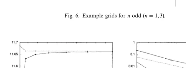
Fig. 7 presents pricing examples for the European put option. The

implemen-tation proceeds as follows: For any re"nementmwe calculate*x

Kby Eq. (25),

which results inj

K"(p/*x

K)by Eq. (23). We calculate the European option

value in a 2Wj

K¹X and a 2Wj

K¹X!1 step binomial model with characteristics

(u

K,dK, 1,qK) and writeUK,2,UK

W_HK2Xto a separate list. Our price

approxima-tion for"xedmis then calculated by Eq. (26). In Fig. 7 we calculated European

Fig. 6. Example grids fornodd (n"1, 3).

Fig. 7. Price, error and bounding error function for a European put.

put option prices iterating over the re"nementsm"1,2, 7. We display them

depending on a"ctitious re"nement of 2Wj

K¹X"18, 78, 178, 316, 494, 712, 970,

since this corresponds to the CRR model which is comparable in terms of the computational cost. On the left-hand we display the values according to the re"nement. The right-hand part contains the absolute di!erence to the true

(continuous time) price.

bounded by the line 1/nfor the RTBM. This suggests that it converges with order one in the"ctitious re"nement 2Wj

K¹X. The following theorem establishes

this result for the RTBM:

Theorem 8. The order of convergence in calculating European call and put option

prices<

Kusing the sequence of RTBM models(SK)Kis one injK:

"<!<

K""_O

j_K

Here<_{denotes the Black}Scholes continuous time solutions (Eqs. (2) and (3)).}

Repeating the derivation of the extrapolation rule (Eq. (16)) in Section 3, using

j_Kinstead ofn, we deduce the following extrapolation rule for RTBM in terms of

the re"nementm:

<

KK" j_K<

K!jK<K j_K!j

K

. (28)

It gives us a way to calculate a new value <

KK from the values <K and

<

Kcorresponding to two re"nementsmandm. Eqs. (27) and (28) con"rm our

remark made in Section 4 that all formulae for CRR hold with the expected time

di!erence 1/j

K.

Fig. 7 also presents the extrapolated values using the sequence (m,m#1).

Please compare with Fig. 2. When we extrapolate our RTBM, we start with very small errors which are almost immediately accurate to the penny. Moreover, extrapolated prices seem to converge with a higher order of two.

A rough cost analysis to evaluate our improvements is the following: To

calculate prices for the standard CRR model with re"nementn, the number of

calculations in the backward induction algorithm is of ordern. The same holds

for our RTBM and its extrapolation, since RTBM and CRR are subject to the same computational cost in calculating prices and extrapolation amounts to a computational cost which is larger only by a constant factor. On the other hand, extrapolation gives the order two. Thus, a rough estimate is

error"O

cost

error"O

cost

These observations make it a powerful pricing tool in the Black}Scholes

5.2. The American put option

In the European option setup, the simple adjustment which led to the SMO yields the same impressive results as our RTBM. We see, however, in this subsection dealing with American options that, in contrast to SMO and CRR, our model is capable of smoothing the American put option and achieves impressive improvements for this case, too.

Similar to Eq. (4), we take for an RTBM with characteristic terms (u

K,dK,qK,jK) the value<Kof the American put as the optimal stopping problem

<

K"sup

NZSK

E[e\PN(K!SK

N )>], (29)

where here SK denotes all stopping times at trading dates adapted to the

"ltration generated by the stock process (SK R )R.

From Lamberton and Page`s (1990) we deduce, checking their condition (H)

by the su$cient conditions of Mulinacci and Pratelli (1998), the following:

Theorem 9. For a sequence of RTBM with *x_KPK 0 and characteristics

(u

K,dK,qK,jK) given by Eqs. (18), (22) and (23), American put option values

<

Kconverge to their price in the Black}Scholes setup.

This consistency result allows calculating continuous-time prices by our

RTBM. De"neWK

L as the value calculated in ann-step binomial model with

characteristic terms (u

K,dK, E[exp+!rq

K,"N2K"n],q

K), according to the

American put backward algorithm presented at the end of Section 2. For

European put options, Eq. (24) shows that the price is a mixture over di!erent

scenarios corresponding to the number of trading dates occurring in the interval

[0,¹], each weighted by its probability. Here we have a similar weighting result

for American options using the termsWK

L .

Proposition 10. Forxxedm,thevalue of the American put option is

<

K"e\HK2

L

(j_K¹)L

n! WLK.

The core of the proof is that conditioning on the (random) number of jumps does not change the value (see also Chow et al., 1991). The implementation is exactly

as in the European put case. However, we calculateW_LK using exp+!r¹/n,

instead of E[exp+!rq

K,"N2K"n]. A series expansion reveals that both are

equal to E[1!rq

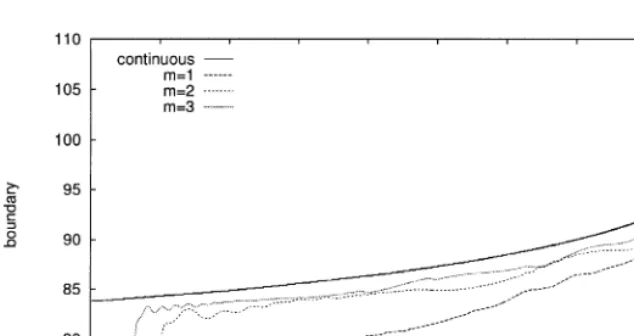
Fig. 8. Boundary approximation.

From each n-step binomial model with characteristic terms (u

K,dK,

exp+!r¹/n,,q

K), a (linearly interpolated) boundaryBKL results. Fig. 8

pres-ents the boundaryBK" WHK2X

L Q[N2K"n]BKL. The discrete boundaryBK

is not completely smooth; however, the overall variation to the continuous boundary over time is reduced. This result is astonishing as the discrete grid is

quite large. For example, form"1 the grid is the same as that in Fig. 4}except

that we have taken here a smaller scale of [75, 110] } and nodes lie at

75.1, 82.6, 90.9, 100, 110. This is in line with our motivation at the end of Section

3 that mixing boundaries resulting from di!erent re"nements would result in

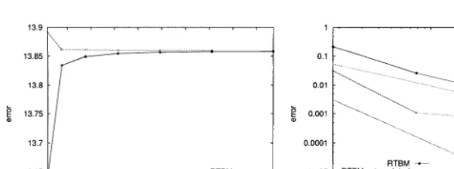
one with a reduced variation and suggests good price approximations. For the American put option, Fig. 9 presents price calculations in the left-hand part and in the right-hand the error to the continuous-time solution. In contrast to the wavy patterns of Fig. 3, here a smooth convergence structure can be seen. Extrapolating our RTBM yields impressive results in terms of accuracy.

We have very small initial errors which give us&penny-accuracy'almost

immedi-ately. Moreover, extrapolated prices seem to converge with a higher order of

two. We would like to point out that } not only for our speci"c one under

consideration}these impressive results hold foranyparameter selection di!

er-ent to SMO.

To compare CRR and RTBM in terms of the computational cost necessary to achieve a certain precision level, note that for CRR the number of calcu-lations and the order needed remain unchanged compared to the European

case (nand order one). However for RTBM we get order two again, but the

number of calculations needed is now of ordern, since all intermediate

Fig. 9 . Price, error and bounding error function for an American put.

rough estimate is

error"O

cost

error"O

cost

In this way, it gives also in the American put option case a very competitive pricing tool, increasing the order with respect to the cost by extrapolation from 1/2 to 2/3.

6. Approximating jump di4usions

This section studies the jump di!usion setup of Merton (1976). Adding the

jump part to the RTBM is straightforward, and we remain in the same frame-work. The simple and competitive valuation tools developed in Section 5 im-mediately apply here.

In an extension of the Black}Scholes model (see Eq. (1)), Merton, 1976

supposed that the stock price can be described by

S R"S

exp+kt#p=

R,,

R

“ G

(1#;

G), (32)

under the objective measure, where the drift k31 is some constant,

(;

G)GZ-L]!1,R[ a sequence of iid random variables and (N

R)R a Poisson

process with intensityj.

SettingX_R"ln(S

R/S), we have

X

R"kt#p=

R#J

where

J R",

R

G

;I

G

and

;I

G"ln(1#;

G). (34)

This setup represents an incomplete market. In the language of Harrison and

Pliska (1981) this means there is no longer a unique equivalent martingale

measure that precludes arbitrage. FoKllmer and Sondermann (1986) speci"ed the

measure that minimizes the writer's risk in some sense. The choice of a

martin-gale measure can also be made by assuming that an exogenously "xed risk

premium is required for the jump risk. Similar to Merton (1976), we assume that

jump risk can be fully diversi"ed and is therefore not priced. The risk-neutral

probability measure is then the one for which k"r!p/2!jE[;

G]. All

valuations are performed with respect to this measure.

Call option values are a mixture of Black}Scholes prices (see Merton, 1976):

e\H2

L

(j¹)L

n! E[C(SZLe\HI2,¹,K,p,r)], (35)

whereC(S

,¹,K,p,r) is the Black_}Scholes formula for call options (Eq. (2)),

k"E[;

G] andZL" “LG

(1#;

G)"exp+ LG

;I G,.

Amin (1993) presents the following extension of the binomial model to deal

with jump di!usions. AsNis a Poisson process with intensityj, the probability

of one jump equalsj*t_Lexp+!j*t

L,on a discrete interval*tL. The probability

of more than one jump is small in comparison to this, and exp+!j*t

L, is

approximately equal to one. Therefore Amin (1993) assumes that between two dates at the most only one jump occurs and that the probability of this event

equals j*t

L. Using a binomial model with grid vL"p(*t

L, iL"k*t

L, he

assumes that jumps occur only to points of this grid. Furthermore, he explains

how to suitably approximate;I

Gby a random variable;I LGwhich takes values at

the grid points at timet

LG only. The returnRMLGis then modelled by

RM LG&

L, (1!j*t

L)qL, i_L!v

L, (1!j*t

L)(1!q

L),

;

LG, j*tL.

()

The probabilityq_Lis set according to Eq. (2) withk"r!p/2!jE[;

G]. Amin

Moreover, although the model is computationally correct, it does not match the idea of a rare event at random time.

For the RTBM corresponding in the jump di!usion setup let us"rst construct

along the lines of Section 4 a sequence (NK,RM

K)K, each element independent of

the other and independent ofNsuch that

,K “ G

R_M

KGN kt#p=

R,

wherek"r!p/2!jE[;

G]. De"ne approximations;I

KGof;I Galong the lines

of Amin (1993), and the process

NM K"N#NK,

which is a Poisson process with intensityjM_K"j#j

K, the sequence of random

variables

Z KG&

KG, j#jj

K

,

RM

KG, j#jKj

K

and the processes

X_M K R ",

M_RK

G

Z

KG and SMRK"expXM K

R .

This has the same structure as the model we constructed in Section 4, and therefore, we call this model also RTBM. We have the following:

Theorem 11. For the RTBM

XM KN X and SMKN S.

The put payo!function is continuous and bounded. This fact, together with

the above theorem and put-call parity, imply:

Proposition 12. The value of European put and call options converge to their

corresponding continuous time solution.

The methods and proofs presented in the previous section immediately carry over:

Proposition 13. The European call and put optionvalue in the RTBM is

<

K"e\P>HMK2

L

(jM_K¹)L

whereU_LKis its price in ann-step tree with characteristic terms(u

K,dK, 1,pK)and the extraordinary jumps u_J

KG.The American put optionvalue is

<

K"e\HMK2

L

(jM

K¹)L

n! WLK,

where W_LK is its price in an n-step tree with characteristic terms (u

K, d

K, E[ exp+!rq

K,"N2K"n],p

K)and the extraordinary jumps uJKG.

Theorem 14. Thevalue of an American put option converges to its continuous-time

solution.

The construction is very easy and straightforward to perform. We believe that it also puts more emphasis on the didactical advantages of the original CRR binomial model. Moreover, we observe in simulations that the remarkable convergence properties of the RTBM carry over to the approximation of jump

di!usions.

7. Conclusion

In this paper we studied a binomial model with random time steps. We

described the di$culties with standard binomial models. We presented a way to

easily calculate price approximations for European and American put and call

options in the Black}Scholes setup and proved convergence to the

continuous-time solution. For European put options, we proved that the order of conver-gence is equal to one. The major contribution lies in a smoothing of the convergence structure for American put options, which allows speed ups by extrapolation: Simulations suggest a much smaller initial constant and order of convergence two. The same holds for American put options. Thus this model

can serve as an e$cient tool in the Black}Scholes setup. A second contribution

is that our model gives intuitive and straightforward approximations to jump

di!usions which seem to preserve the outstanding properties.

Acknowledgements

The author is grateful to Damien Lamberton, Klaus SchuKrger, Dieter

Sonder-mann and to the referees. They greatly improved the exposition and the motivation for this paper. Financial support from the Deutsche Forschun-gsgemeinschaft, Sonderforschungsbereich 303 at Rheinische

Appendix A. Proofs

In contrast to the common literature, this paper de"ned the CRR model on

the whole interval [0,¹] instead of only at datest

LG3_TL. This is for technical

convenience and as long as we restrict trading dates to the discrete setTL, this

makes no di!erence. The processes we study are processes whose paths are

continuous to the right, but have left-side limits (called ca%dla%gprocesses). We

will further suppose that the spaceDof ca`dla`g processes is equipped with the

Skorohod topology and denote byN the weak convergence on D.

Proof of Theorem 1.The proof of the"rst assertion is an application of Donsker's

theorem in a suitable form for our case (see Corollary VII.3.11 in Jacod and

Shiryaev, 1987). Please note that we only need to check the"rst two moments.

The second assertion follows from the observation that the exponential function is continuous.

Proof of Theorem 2. Necessary conditions include convergence of the "rst

moment to its continuous value E[X

R]"(r!p/2)tand of the second moment

to Var(X

R)"pt. We denote for t'0 k

K(t)"E[NK

R ,"j

Kt. For the "rst

moment, using the Wald equality, we have

E[X_M K

R ]"E

K

R

G

R_M K

"E[NK

R ]E[RMK]

"k

K(t)E[RM KG].

We have

E[(XM K

R )]"E

K

R

G

RM KG

"E

K

R

G

(RM

KG)#,

K

R

G

,_RK HH$G

RM KGRMKH

"E

K

R

G

(RM

KG)#,

K

R

G

,_RK HH$G

RM

KGRMKH

Due to the independence of (NK)_Kand (RM_KG)_KG, this can be simpli"ed to

L

P[NK

R "n]E

G

(RM

KG)# L

G

L HH$G

RM KGRMKH

"

L

P[NK

R "n](nE[(RM

KG)]#n(n!1)E[RM

The previous result implies

Var(XM _RK)"E[(XM K

R )]!E[XM K

R ]

"E[(XM K

R )]!(k

K(t)E[RMK])

"k

K(t)E[(RM K)]#E[(NK

R )]E[RMK]

!k

K(t)E[RMK]!(k

K(t))E[RMK]

"k

K(t)Var(RMK)#E[RM

K] .

As Var(N_RK)"k

K(t)"j

Kt, we conclude with the result on the "rst moment

(Eq. (19)). 䊐

Proof of Theorem 3. Let us de"ne (depending on m) the two sequences of

processes (M_RK)_Rand (A_RK)_Rby

MK R ": ,

K

R

G

lnR_M

KG!

2

AK R :"pt.

Then, for eachm, the processes (MK

R )Rand ((MRK)!AK

R )Rare martingales. As

the jump sizes are of order v

L and vanish in the limit, we deduce from the

Martingale Central Limit Theorem as stated in Ethier and Kurtz (1986) that

MN p=. 䊐

Proof of Theorem 8.Similar to Leisen and Reimer (1996), we de"ne the (pseudo-)

moments

m_KL": E

K,!SOK

S

N₂K"n

m_KL": E

K,)!

S

m

KL": E

K,)!

S

p

K": E[(RM

K)(exp+RMK,!1)],

which are the structural properties of the RTBM under consideration. Now, the proof is just the application of a general technique to derive error bounds (see

Kloeden and Platen, 1992). For binomial models in the Black}Scholes setup, it

<!<

K"

LP[N2K"n])(<!e\P2UK

L ), the proof proceeds on

<!e\P2UK

L exactly as in their paper. We sketch the main ideas: A

Taylor-series expansion up to terms of order three yields terms of structure (l"1, 2, 3):

L

P[N₂K"n]mJK

LL\ I

e\POI>E

I )J

*J<

*SJ (qLI>,SMOKI)

L

P[NK

2 "n]L\

I

e\POI>E[R(qLI>

,SMOKI>,SMOKI)"N2K"n],

whereRis a remainder term.

It remains to prove that the terms L_I\2(l"1, 2, 3) are of orderO(n), and

the summation over the remainder is of orderO(np

K). The proof concludes by

checking that the (pseudo-)moments have the right order: It is easy to see that

p

K"O(1/j

K). Furthermore, for the l"1 term this can be calculated in

a straightforward way using E[R_M

K]"1#r¹/j

K#_O(1/j

K) and

E[S

OK/S"N2K"n]"1#r¹/n#O(1/n). All others can be derived

immediate-ly from this by appimmediate-lying the method in Appendix B of Leisen and Reimer

(1996). 䊐

Proof of Proposition 10.The proof is independent of any speci"c choice onm. To

ease exposition we will therefore omit any dependence onm. For anyt3[0,¹],

denote by F_R"p(SM

RY"t4t) the "ltration corresponding to the information

observing the discrete processSM, and bySthe stopping times which are adapted

to the"ltration (F

R)R and take values at trading dates before¹. We refer the

current time after theith jump has occurred byq

G" GH

qH.

We"rst prove the theorem in the case where the numberN

2of jumps on the

interval [0,¹] is bounded by someM3-. In a second step we will prove it in its

full generality through a limit argumentMPR. Fix oneM3-. We study

the driving process N+"min+N,M,,

and the process SM+",

+

“ G

exp+RM G,,

as well as the"ltration (set of stopping times)F+

R "p(SM+

RY"t4t) (S+)

corre-sponding to the information observing SM+, F,+

R "p(SM+

RY,N+2"t4t) (S,+)

corresponding to the information observingSM+and knowingN

2, andFLR+"

F+

R R+N2"n,(SL+) corresponding to the information that results from the

observation ofSM +, and when it is known thatnjumps will occur in total on the

interval [0,¹].

For"xedM, we de"ne a correspondencepp,between the stopping times

p3S+andp,3S,+such that both yield the same expected payo!as exercise

policy; i.e., for anyp,3S,+we assign ap3S+such thatpN+