www.ann-geophys.net/30/639/2012/ doi:10.5194/angeo-30-639-2012
© Author(s) 2012. CC Attribution 3.0 License.
Annales
Geophysicae
A meteor head echo analysis algorithm for the lower VHF band
J. Kero1,2, C. Szasz1, T. Nakamura1, T. Terasawa3, H. Miyamoto4, and K. Nishimura1
1National Institute of Polar Research (NIPR), 10-3 Midoricho, Tachikawa, 190-8518 Tokyo, Japan 2Ume˚a University, Box 812, 981 28 Kiruna, Sweden
3Institute for Cosmic Ray Research, Univ. of Tokyo, 5-1-5 Kashiwa-no-ha, Kashiwa city, 277-8582 Chiba, Japan 4Department of Earth Science and Astronomy, College of Arts and Sciences, Univ. of Tokyo, Komaba 3-8-1, Meguro-ku,
153-8902 Tokyo, Japan
Correspondence to: J. Kero ([email protected])
Received: 17 July 2011 – Revised: 3 January 2012 – Accepted: 13 March 2012 – Published: 2 April 2012
Abstract. We have developed an automated analysis scheme for meteor head echo observations by the 46.5 MHz Mid-dle and Upper atmosphere (MU) radar near Shigaraki, Japan (34.85◦N, 136.10◦E). The analysis procedure computes
me-teoroid range, velocity and deceleration as functions of time with unprecedented accuracy and precision. This is crucial for estimations of meteoroid mass and orbital parameters as well as investigations of the meteoroid-atmosphere interac-tion processes. In this paper we present this analysis proce-dure in detail. The algorithms use a combination of single-pulse-Doppler, time-of-flight and pulse-to-pulse phase cor-relation measurements to determine the radial velocity to within a few tens of metres per second with 3.12 ms time resolution. Equivalently, the precision improvement is at least a factor of 20 compared to previous single-pulse mea-surements. Such a precision reveals that the deceleration increases significantly during the intense part of a meteor-oid’s ablation process in the atmosphere. From each received pulse, the target range is determined to within a few tens of meters, or the order of a few hundredths of the 900 m long range gates. This is achieved by transmitting a 13-bit Barker code oversampled by a factor of two at reception and using a novel range interpolation technique. The meteoroid veloc-ity vector is determined from the estimated radial velocveloc-ity by carefully taking the location of the meteor target and the an-gle from its trajectory to the radar beam into account. The latter is determined from target range and bore axis offset. We have identified and solved the signal processing issue giving rise to the peculiar signature in signal to noise ratio plots reported by Galindo et al. (2011), and show how to use the range interpolation technique to differentiate the effect of signal processing from physical processes.
Keywords. Interplanetary physics (Interplanetary dust) – Ionosphere (Instruments and techniques) – Radio science (Instruments and techniques)
1 Introduction
The flux of meteoroids onto Earth is the source of the neutral and ion metal layers in the middle atmosphere. The influx plays an important role in atmospheric dynamics and pro-cesses like the formation of high-altitude clouds, possibly through coagulation of meteoric smoke particles acting as condensation nuclei for water vapor (Summers and Siskind, 1999; Megner et al., 2006). Hunten et al. (1980) point out that estimating the deposition of mass in the atmosphere re-quires knowledge of not only the total mass influx of mete-oroids, but also the size and velocity distributions and phys-ical characteristics such as density and boiling point of the particles.
Meteor head echo observations with High-Power Large-Aperture (HPLA) radars are well suited for studying many aspects of the meteoroid influx in detail, as well as the atmo-sphere interaction processes (e.g. Pellinen-Wannberg, 2005). Meteor head echoes are radio waves scattered from the in-tense regions of plasma surrounding and co-moving with meteoroids during atmospheric flight. Head echoes were first reported by Hey et al. (1947), who observed the Gia-cobinid (now called Draconid) meteor storm of 1946 with a 150 kW VHF radar. HPLA radar systems, however, have a peak transmitter power of the order of 1 MW and ar-ray or dish antenna apertures in the range of about 800– 7×10⁴m2 (Pellinen-Wannberg, 2001), focusing their an-tenna gain pattern into a narrow main beam with a full-width-at-half-maximum (FWHM) of the order of 1◦ at the VHF
and/or UHF operating frequencies. This high power density permits numerous head echo detections from faint meteors.
2011). These radar systems have diverse system character-istics in terms of operating frequency, dish or phased array antenna, aperture size etc. Characteristics of all but the Res-olute Bay Incoherent Scatter Radar (RISR) are summarized in Table 1 of Janches et al. (2008). Methods of head echo analysis have been developed more or less independently at several of the facilities, and with emphasis on different as-pects of meteor science and/or radio science issues. In Sect. 2 we give a brief review of references to previously developed meteor head echo analysis methods, and point out new fea-tures in our approach.
We have developed and implemented an automated anal-ysis scheme for meteor head echo observations by the 46.5 MHz Middle and Upper atmosphere (MU) radar near Shigaraki, Japan (34.85◦N, 136.10◦E) (Fukao et al., 1985). Previous meteor head echo observations with the MU radar have been reported by Sato et al. (2000) and Nishimura et al. (2001).
The algorithms presented here use a combination of single-pulse-Doppler, time-of-flight and pulse-to-pulse phase correlation measurements, enabling the meteoroid ra-dial velocity to be determined to within a few tens of m s−1 with 3.12 ms time resolution. Equivalently, the precision improvement of the determined line-of-sight velocity is at least a factor of 20 compared to previous single-pulse mea-surements. Furthermore, we have invented an interpolation scheme to find the target range within a small fraction of the 900 m long range gates. This, together with the upgrade of the MU radar receiver system from four analog to 25 digital channels (Hassenpflug et al., 2008), results in improved tar-get position determination, crucial for accurately estimating meteoroid trajectory parameters and calculating true meteor-oid velocities from the measured radial velocity component along the radar line-of-sight.
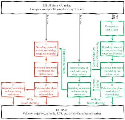
A block diagram of the analysis scheme is shown in Fig. 1. The paper is organized to describe the blocks as follows.
A brief description of the MU radar and our experimental settings is found in Sect. 3. The initial search for meteor events (block A) and an overview of the decoding proce-dure (block B) is given in Sect. 4. The new range interpo-lation technique is presented in Sect. 5. It solves a major and systematic signal processing issue in meteor head echo data (Galindo et al., 2011), further discussed in Sect. 5.1. The se-lection of data points constituting one meteor event (block C) is described in Sect. 6. These data points are then subject to the pulse-to-pulse phase correlation technique (block D) re-ported in Sect. 7.
The instantaneous position of a meteor target at each inter-pulse period (IPP) is determined by interferometry (block E) using the MUSIC method (Schmidt, 1986) explained in Sect. 8. Meteoroid trajectories and radiant error estimations are determined by combining the interferometry data with the estimated range data and the radial velocity (block F) as detailed in Sect. 9. In turn, the trajectories are used to redo the parts of the analysis given in blocks B–D, but with the
re-ceiver beam post-steered towards the most probable location of the meteor target at each IPP.
In Sect. 10 we present meteor target radar cross section (RCS) calculations. Comparing the RCSs with and without post-steering the receiver beam gives an estimate of the va-lidity of the position determination and the applied antenna gain pattern. To ensure as accurate position determination as possible, we have adopted an interchannel calibration rou-tine, described in Sect. 11.
The analysis output parameters are range, altitude, radial velocity, meteoroid velocity, instantaneous target position, RCS and meteor radiant. The parameter values calculated both with and without using post-beam steering are stored in a data base.
2 Meteor analysis methods at other HPLA radars
Evans (1965, 1966) describes the first head echo measure-ments with what today is termed a HPLA radar. He used the 440 MHz Millstone Hill radar, which has an operating frequency about an order of magnitude higher than classical specular meteor trail radar systems. Evans maximized the cross-beam detection area of the Geminid, Quadrantid and Perseid meteor showers by pointing the Millstone Hill radar towards the shower radiants at times when the radiants were located at very low elevations above the local horizon. This enabled velocity and deceleration determination for meteors belonging to the showers, for which the atmospheric trajec-tories were aligned with the radar beam.
2.1 EISCAT
INPUT from MU radar:
Complex voltages, 85 samples every 3.12 ms
OUTPUT:
Velocity, trajectory, altitude, RCS, etc. with/without beam steering
A. Eventsearch:
scan of data
B. Decoding potential
events, optimizing range and Doppler
C. Selecting data points
constituting one meteor event
D. Pulse-to-pulse phase
correlation of selected data
Raw
data
Optimal range values
for selected IPPs
Radial
velocity
Without beam steering E.
Interferometry of each echo using range values
F.
Trajectory calculation and uncertainty
estimation
Raw data
Beam steering vaules
B. Decoding potential
events, optimising range and Doppler
C. Selecting data points
constituting one meteor event
D. Pulse-to-pulse phase
correlation of selected data
Raw data
With beam steering F.
Trajectory calculation and uncertainty
[image:3.595.93.500.61.450.2]estimation
Fig. 1. Block diagram of the analysis scheme.
detailed description of this improvement and the signal pro-cessing development following the installation of the new digital signal processing and raw data recording systems in 2001, which enabled phase-coherent pulse-by-pulse analysis. Kero et al. (2008a) present a method for finding the posi-tion of a compact meteor target in the common volume mon-itored by the three UHF receivers, and how velocity, decel-eration, RCS and meteoroid mass were estimated from the improved tristatic observations. The EISCAT UHF radar pro-vided excellent precision and accuracy of meteors observed with all three widely separated receiver systems, but low rate of such events ('10 h−1), mainly due to the small tristatic measurement volume (Szasz et al., 2008).
2.2 AO
Zhou et al. (1995) observed the first head echoes using the Arecibo Observatory (AO) 430 MHz UHF radar. The ob-servations were limited to time integrated data and a time
resolution of 11 s. Mathews et al. (1997) followed up the AO observations with an improved non-integrated data col-lection approach, enabling 1 ms time resolution. The ler technique for obtaining the instantaneous meteor Dopp-ler velocity and deceDopp-leration is described in Janches et al. (2000a,b, 2001). Subsequent improvement of the signal pro-cessing techniques at AO has been particularized by Math-ews et al. (2003); Wen et al. (2004, 2005a); Briczinski et al. (2006); Wen et al. (2005b, 2007). The emphases of the anal-ysis technique development have been to implement auto-mated real-time analysis of meteor parameters (Wen et al., 2004), remove non-periodic bursty interference (Wen et al., 2005b), and separate incoherent scatter from meteor signals (Wen et al., 2005a, 2007).
2.3 ALTAIR
Tracking and Instrumentation Radar (ALTAIR) to calculate atmospheric meteoroid trajectories of meteors observed dur-ing the 1998 Perseid meteor shower, and durdur-ing the 1998 Leonid meteor storm (Close et al., 2002). No conclusive evidence of shower meteor detections were found, in accor-dance with the (subsequently estimated) very low probabil-ity of detecting such meteors during the observations (Brown et al., 2001).
Close et al. (2005) present a method for meteoroid mass estimation by converting the measured RCS to head echo plasma density utilizing a spherical electromagnetic scatter-ing model. The ALTAIR radar has multi-frequency capa-bility, and can transmit linear frequency modulated chirped pulses. This enables a variety of meteoroid range rate calcu-lations, e.g. based on the difference in the measured ranges due to range-Doppler coupling (Loveland et al., 2011). 2.4 PFISR, SRF and RISR
Mathews et al. (2008) applied the analysis methods devel-oped for the 430 MHz AO radar and described by Mathews et al. (2003) and Briczinski et al. (2006), to the 449.3 MHz 32 panel Advanced Modular Incoherent Scatter Radar at Poker Flat Alaska (PFISR-32), to the 1290 MHz Sondre-strom Radar Facility (SRF), and later also to the Resolute Bay Incoherent Scatted Radar (RISR) (Malhotra and Math-ews, 2011).
Mathews et al. (2008) estimated that AO is 77 times more sensitive than SRF and 2100 times more sensitive than PFISR. Yet, they found the lowest event rate at SRF (34 per hour) relative to PFISR (55 per hour) and AO (1000 per hour). Furthermore, the altitude distribution of SRF mete-ors was 10 km below that observed with AO/PFISR. These observations agree with a frequency dependent meteor head echo target RCS, further discussed in Sect. 10, as well as the cut-off in the high-altitude end of the 930 MHz EISCAT UHF distribution as compared to the 224 MHz EISCAT VHF distribution (Westman et al., 2004).
Sparks et al. (2009) report the results of concurrent PFISR observations using an independent but similar data analysis method. (Sparks et al., 2010) operated PFISR as a three-channel interferometer. They demonstrate that meteor radi-ants and orbits can be determined.
Chau et al. (2009) describe an antenna compression ap-proach to widen the PFISR beam width for meteor head echo observations, to about three times the width of the ordinary narrow beam. Chau et al. corrected the signal-to-noise ratio (SNR) depending on where in the beam meteors were de-tected, thus estimated a corrected relative RCS distribution, i.e. as if all meteors were detected within the narrow main lobe. Using a wider beam to detect a larger number of strong and/or long-duration meteor head echo events, which would not have been detected in the narrow beam, is an interesting and promising approach. However, it is not a necessary
pro-cedure to enable beam shape correction for interferometric observations with the MU radar.
2.5 JRO
Chau and Woodman (2004) and Chau et al. (2007) used the 50 MHz Jicamarca Radio Observatory (JRO) radar for me-teor head echo observations. They utilize three-channel in-terferometry to calculate meteoroid trajectories and convert the radial velocity to vector velocity. 13-bit Barker coded pulse sequences were transmitted to decrease interference from geophysical clutter, and pulse-to-pulse phase correla-tion was used to estimate radial deceleracorrela-tion. The sampling rate was equal to the subpulse (baud) rate (Chau et al., 2007, Table 1). Chau and Galindo (2008) report the first interfer-ometric head echo observations of meteor shower particles. Galindo et al. (2011) describe a signal processing issue in JRO data that manifests itself as a peculiar signature in SNR plots.
2.6 Discussion
The outline of the analysis technique presented in this paper is similar to that presented by Chau and Woodman (2004) for interferometric JRO observations. The way target range and Doppler velocity are extracted from the raw data in a multi-step matched-filter procedure (Sects. 3–4) largely fol-lows the EISCAT analysis technique detailed by Wannberg et al. (2008) and Kero et al. (2008a).
The first main difference between the method at hand and published methods is that we have developed a range finding interpolation technique for BPSK (binary phase-shift key) coded pulse sequences (Sect. 5). This technique solves the systematic signal processing issue causing ripples in the JRO data reported by Galindo et al. (2011). Also, Chau and Woodman (2004) report that there is a bias between the JRO time-of-flight velocity estimation and Doppler estimation. Our determined radial velocity component (Sect. 3, Fig. 5) is unbiased, similarly to EISCAT observations (Wannberg et al., 2008).
The third main difference is that we have implemented in-terferometry utilizing all 25 channels of the MU radar re-ceiver system (Sect. 8), enabling unambiguous target local-ization. Three receiver channels were used for interferomet-ric JRO observations (Chau and Woodman, 2004), as well as previous interferometric MU observations (Nishimura et al., 2001). Three channels are, in principle, enough to locate me-teors inside the transmitter beam, but Chau et al. (2009) note that more than three antennas are required to remove angular ambiguities as a significant fraction of the meteors appear in sidelobes.
The fourth principal difference is the way we convert ra-dial velocity to vector velocity (Sect. 9). Equation (4) in Chau and Woodman (2004) is a good approximation, but does not utilize all information of a meteor event.
Improving the accuracy and precision of meteoroid veloc-ity vector determination in head echo observations is impor-tant to provide useful data for the modelling of Solar System dust, e.g. for studying the evolution of meteoroid streams and predicting meteor shower outbursts (Jenniskens, 2006; Sato and Watanabe, 2007; Atreya et al., 2010).
3 The MU radar experimental setup
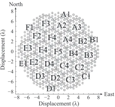
The present setup of the MU radar hardware comprises a 25 channel digital receiver system. It was upgraded from the original setup (Fukao et al., 1985) in 2004 and is described by Hassenpflug et al. (2008). After the upgrade, the MU radar always transmit right-handed circular (RC) polarization and receive left-handed circular (LC) polarization, with a phase accuracy of 2◦. The output of each digital channel is the sum of the received radio signal from a subgroup of 19 Yagi an-tennas. The whole array consists of 475 antennas, evenly distributed in a 103 m circular aperture. A schematic view of the array and the subgroups is given in Fig. 2. It is pos-sible to combine the output from several subgroups into the same digital channel to reduce the total number of channels and hence decrease the data rate without decreasing the total aperture. We have, however, chosen to use all 25 channels to enable subgroup phase offset reduction and to optimize in-terferometric target position determination and post-steering of the receiver beam. The maximum continuous data rate is about 20 GB h−1due to system limitations.
The range finding interpolation algorithm works best if the transmitted code is selected as to have a minimum value next to the central maximum in its autocorrelation function (ACF). The autocorrelation of a 13-bit Barker code has zeros next to the central peak. This property maximizes the preci-sion of the range interpolation for a given code length. Other properties of the transmission schedule as the number of bits in the code, baud length, IPP, etc., are not restricted by the range finding interpolation algorithm and should be chosen according to hardware limitations and other constraints.
−8 −6 −4 −2
0
2
4
6
8
−8
−6
−4
−2
0
2
4
6
8
Displacement (λ)
Displacement (λ)
1 2 3 4 5 6 7 8 9 10 11 12 13 14 15 16 17 18 19 1 2 3 4 5 6 7 8 9 10 11 12 13 14 15 16 17 18 19 1 2 3 4 5 6 7 8 9 10 11 12 13 14 15 16 17 18 19 1 2 3 4 5 6 7 8 9 10 11 12 13 14 15 16 17 18 19 1 2 3 4 5 6 7 8 9 10 11 12 13 14 15 16 17 18 19 1 2 3 4 5 6 7 8 9 10 11 12 13 14 15 16 17 18 19 1 2 3 4 5 6 7 8 9 10 11 12 13 14 15 16 17 18 19 1 2 3 4 5 6 7 8 9 10 11 12 13 14 15 16 17 18 19 1 2 3 4 5 6 7 8 9 10 11 12 13 14 15 16 17 18 19 1 2 3 4 5 6 7 8 9 10 11 12 13 14 15 16 17 18 19 1 2 3 4 5 6 7 8 9 10 11 12 13 14 15 16 17 18 19 1 2 3 4 5 6 7 8 9 10 11 12 13 14 15 16 17 18 19 1 2 3 4 5 6 7 8 9 10 11 12 13 14 15 16 17 18 19 1 2 3 4 5 6 7 8 9 10 11 12 13 14 15 16 17 18 19 1 2 3 4 5 6 7 8 9 10 11 12 13 14 15 16 17 18 19 1 2 3 4 5 6 7 8 9 10 11 12 13 14 15 16 17 18 19 1 2 3 4 5 6 7 8 9 10 11 12 13 14 15 16 17 18 19 1 2 3 4 5 6 7 8 9 10 11 12 13 14 15 16 17 18 19 1 2 3 4 5 6 7 8 9 10 11 12 13 14 15 16 17 18 19 1 2 3 4 5 6 7 8 9 10 11 12 13 14 15 16 17 18 19 1 2 3 4 5 6 7 8 9 10 11 12 13 14 15 16 17 18 19 1 2 3 4 5 6 7 8 9 10 11 12 13 14 15 16 17 18 19 1 2 3 4 5 6 7 8 9 10 11 12 13 14 15 16 17 18 19 1 2 3 4 5 6 7 8 9 10 11 12 13 14 15 16 17 18 19 1 2 3 4 5 6 7 8 9 10 11 12 13 14 15 16 17 18 19North
East
A1
A2 A3
A4
B2
B1
[image:5.595.311.547.61.281.2]B3
B4
C1
C2
C3
C4
D1
D2
D3
D4
E1 E2
E3 E4
F1
F2
F3
F4
F5
Fig. 2. A schematic view of the MU radar antenna array. It con-sists of 475 antennas arranged in a grid of equilateral triangles with
an element spacing of 0.7λ(Fukao et al., 1985). The array is
di-vided into 25 subgroups (A1-F5), each consisting of 19 antennas and connected to its own transmitter and receiver module (Has-senpflug et al., 2008).
However, the implementation described in Sect. 5 is de-signed for a radar setup where the transmitted pulse sequence is oversampled at reception. In the present MU observations it was oversampled by a factor of two, accomplished by using a sampling period ofTs=6 µs while transmitting the Barker
code with a 12 µs baud length. The MU radar hardware does not allow receiver sampling period and transmitter subpulse length to differ. Each 12 µs baud of the 13-bit code is there-fore defined as two 6 µs subpulses of equal phase in the radar experimental setup definition file. The transmitter and re-ceiver bandwidths are defined by the 6 µs subpulse length and the 6 µs sampling period, and approximately equal to
bw=1/6 µs'167 kHz. In the decoding procedure we use
an ideal, boxcar version of the transmitted code pattern, as exemplified in Fig. 3, and further described in Sect. 5 and by Eq. (3).
0
5
10
15
20
25
−1
0
1
Bit no of code
0
10
20
30
40
50
0
10
20
30
[image:6.595.309.549.61.298.2]Autocorrelation of code
Fig. 3. A representation of a 13-bit Barker code oversampled by a factor of two used in the described MU radar experimental setup (upper panel) and its ACF (lower panel).
−180 −120 −60 0 60 120 180 −35
−30 −25 −20 −15 −10 −5 0
Frequency [kHz]
Power [dB]
−40
Fig. 4. Power frequency spectrum of the transmitted code (blue), the receiver bandwidth (red), the received spectrum of a meteor with zero radial velocity (green), and the spectrum of a meteoroid with
70 km s−1radial velocity (black), corresponding to a Doppler shift
of 21.7 kHz.
However, the slight loss of received energy is asymmet-ric, as can be seen in Fig. 4. To confirm the validity of our Doppler estimates, Fig. 5 displays a comparison to indepen-dent time-of-flight estimates. They agree to within the order of one part in a thousand. This comparison demonstrates that the small but asymmetric loss of spectral energy does not bias the Doppler estimation of the velocity. Furthermore, the result agrees with the investigation by Wannberg et al. (2008), who found that no contribution from slipping plasma could be detected within the measurement accuracy of the EISCAT UHF meteor observations, and that the Doppler ve-locities were unbiased. Doppler and time-of-flight methods are further described in Sect. 5.
0
10
20
30
40
50
60
70
0
10
20
30
40
50
60
70
Time−of−flight velocity [km/s]
[image:6.595.51.285.62.255.2]Doppler velocity [km/s]
Fig. 5. Doppler velocity versus time-of-flight velocity for>100 000 MU radar meteors. The solid line is a linear least-squares-fit with a
slope of'0.998.
The selection of a 156 µs pulse length and 6 µs sampling is a tradeoff between time resolution, range resolution, signal-to-noise ratio (SNR) and the maximum possible data rate at the present MU radar system. A longer pulse length would indeed improve the SNR but also increase the time between consecutive pulses due to the 5 % transmitter duty cycle lim-itation.
A longer pause between pulses has two drawbacks; it in-creases the ambiguity of velocity data calculated from pulse-to-pulse phase correlations (cf. Sect. 7) and decreases the time resolution of the determined meteoroid parameters for one and the same meteor event. We have tried several dif-ferent setups in search for a good tradeoff and found that increasing the IPP beyond∼3 ms complicates the selection procedure of a velocity for the meteoroid among ambiguous possibilities determined by pulse-to-pulse phase correlation, described further in Sect. 7. The IPP we finally decided for,
Tipp=3.12 ms, gives a separation1vequal to
1v= λ 2Tipp
'1034 m s−1 (1)
between possible ambiguous velocities.
[image:6.595.50.288.319.460.2]4 Initial analysis: range and Doppler
The meteor head echo analysis procedure starts with a simple scan of the data. It is similar to the meteor data analysis per-formed on EISCAT VHF and UHF radar data described by Wannberg et al. (2008) and Kero et al. (2008a). The scanning procedure performs a search in the power domain by com-puting the boxcar function of 26 consecutive range gates (the length of a point target echo) and compares the result to the noise. If the boxcar function of seven consecutive IPPs ex-ceed three noise standard deviations, the IPPs are flagged as a possible event. This choice of threshold keeps the number of false events at a reasonably low level without excluding analysable meteor head echoes.
An estimate of a meteoroid’s radial (line-of-sight) velocity
vrcan in principle be deduced using the Doppler shiftfDof
one single received radar pulse as the Doppler shift depends on meteoroid velocity and operating frequencyf0according
to
fD=
2f0vr
c0
, (2)
wherec0is the speed of light.
When a meteoric particle enters the atmosphere it will heat up in collisions with atmospheric constituents and generate a dense ionized plasma, generally detectable by radar along several kilometer of its trajectory, before the particle van-ishes. To determine whether an enhanced signal in the data is due to a meteor target or not, we require the target time-of-flight velocity to agree with its Doppler shift. For this criterion to be applied, several IPPs worth of data needs to be recorded from each meteor. This is easily achievable with an IPP of 3.12 ms but demands precise range data. One range gate is defined by the sampling period, which in our obser-vations equals an extent in range of aboutRs=Tsc0/2'
900 m. Our range finding interpolation algorithm enables a time-of-flight velocity calculation even when the meteor tar-get is within one and the same range gate for the duration of the event.
Whenever there are several possible events with gaps smaller than 20 IPPs (62 ms) between them, we try treat-ing them as one streat-ingle meteor and analyze the whole set of IPPs together. Shorter gaps are, in case of MU meteor head echoes, most often caused by one meteor target of low SNR with an irregular ionization/RCS profile or moving through a minimum in the antenna radiation pattern.
Instead of limiting the temporal extent of a meteor event by a threshold on the signal and use all received radar pulses in between for determining meteor properties we have devel-oped an automatic routine that looks for consistency in both velocity versus time and range versus time. Data points that do not fulfil the criteria are excluded. By looking for consis-tency we also try to include data points from before and after the initially flagged sequence of IPPs. Therefore, the interval
Radar pulse
Range gate
20 40 60 80 100
10 20 30 40 50 127 km = 60 70 80
73 km = 0
Head echo
26 samples
Blackout due to out-of-phase
[image:7.595.311.547.60.250.2]reception
Fig. 6. Range-time and signal intensity plot of a meteor head echo event detected 28 July 2009, 05:33:09 JST, in subsequent figure cap-tions and the text referred to as “meteor 1”.
that we analyze and look for consistency within include 20 IPPs before and after the marked sequence.
In the second step of the analysis procedure the 85 range gates from one transmission/reception is cross-correlated with a set of differently Doppler-shifted versions of the trans-mitted code in order to find an approximate Doppler shift and range of the echo. The unshifted code can be described as
Ak(k=0,1,...,27)= (3) [0,+1,+1,+1,+1,+1,+1,+1,+1,+1,+1,−1,−1,−1,
−1,+1,+1,+1,+1,−1,−1,+1,+1,−1,−1,+1,+1,0],
where the zero elements in both ends represent start and stop of transmission. These zero elements are necessary to de-fine for the code sequence to be used successfully in the range finding interpolation technique described in Sect. 5. The ideal version of the code illustrated in Fig. 3 is Doppler-shifted by the multiplication
Bk=Akei2π fnTsk (k=0,1,...,27), (4)
where the Doppler frequency fn= −30 000, −29 000, ..., 5000 Hz andTs=6 µs.
The first guess of Doppler and range is done by select-ing the Doppler frequency givselect-ing the highest peak decoded power and picking out the 26 + 1 range gates that correspond to the location of the highest peak in the cross-correlation for further analysis.
5 Range finding interpolation
a
b a b a b
0 5 10 15 20 25
−1.0 −0.5 0 0.5 1.0
Bit of code 0 5 10Bit of code15 20 25 0 5 10Bit of code15 20 25
0 10 20 30 40 50
0 5 10
Cross−correlation with Doppler−shifted code
0 10 20 30 40 50
Cross−correlation with Doppler−shifted code
0 10 20 30 40 50
Cross−correlation with Doppler−shifted code
0 10 20 30 40 50
0 5 10
Cross−correlation with interpolated Doppler−shifted code
0 10 20 30 40 50
Cross−correlation with interpolated Doppler−shifted code
0 10 20 30 40 50
Cross−correlation with interpolated Doppler−shifted code ⎪
⎪ ⎪
⎩ ⎪⎪ ⎪
⎨ ⎧
− → ≥
− → <
2 1 2 1
a b b a
b a b a
−1.0 −0.5 0 0.5 1.0
0 5 10
0 5 10
Decoded power
Decoded power
Interpolated code
Decoded power
Decoded power
[image:8.595.48.549.61.403.2]Interpolated code
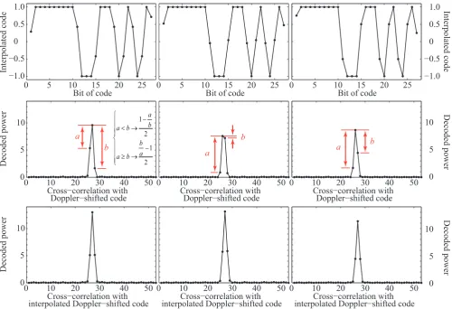
Fig. 7. The interpolated code (top), the cross-correlation with a Doppler-shifted code (middle), and the cross-correlation with the interpolated Doppler-shifted code (bottom) of IPP 72 (left column), IPP 74 (middle column) and IPP 76 (right column) of meteor 1. The interpolated
codes correspond to1=0.287,1= −0.477 and1= −0.248, respectively.
few hundredths of a range gate. The twofold oversampling of the transmitted BPSK coded sequence means that the two range gates next to the peak in the cross-correlation sequence will in ideal cases have half the value of the peak, as was il-lustrated in Fig. 3.
The relation between sampling with a sampling period of
Tsand target rangeris
r=r0+
(gr+1)Tsco
2 , (5)
wherer0is the target range at start of sampling (in the
de-scribed observationsr0≈72 km), gr is the integer number
of range gates (each of lengthTsco/2'900 m) and1is the
remaining fraction of a range gate. The decoded signals(r)
will be symmetric with respect to a particular range gate (rg),
if and only if the target is located at a distance corresponding to an integer number of sampling periods from the radar, thus
1=0. If the target location, however, is such that16=0 the signals(r)becomes asymmetric. The ratio of the values next
to the peak of the decoded power can be used to estimate1
according to
a < b→1=1 −a
b
2 a≥b→1=
b a−1
2 , (6)
whereaandb are the differences between the peak and the adjacent range gates (illustrated in Fig. 7 described below). We use the value11 from the first decoding attempt to
se-lect the 26 + 1 range gates containing the echo. Then we start an iterative procedure in which at each step a new value1n
is calculated at the same time as the Doppler shift used for decoding the signal is optimized. The optimization is ac-complished by first increasing the Doppler shift with a given step size, and evaluate the cross-correlation until the decoded power is smaller than the previous value. At this point the step size is decreased and the search direction is reversed. The procedure is iterated until the step size is 5 Hz, corre-sponding to about 20 m s−1.
of symmetry and the value of the peak decoded power. Op-timization of the two quantities are therefore searched for si-multaneously. Each time a step is taken in Doppler frequency and a new cross correlation is computed, the new ratio1nis
added to form a sum of all evaluations according to
1= m X
n=1
1n. (7)
Generally, the absolute value |1n| in each new iteration is
smaller than the previous value. The sum thus forms a con-verging series, wheremis the number of iterations. The sign of each1ndepends on which ofaandb that are greater in
that particular iteration.
The interpolated codes are found by adding zeroes to each end of the original 26 bit long code, as shown in Fig. 3, and thereafter interpolate adjacent bits of code.1=0 means that bit 1–26 of the code in Fig. 3 are used. If1 <0, interpola-tion is performed towards left (bit 0) and if1 >0 towards right (bit 27). It should be noted that 1= ±0.5 gives rise to zeros when the interpolation is performed on consecutive values of+1 and−1 (or−1 and+1). This is obvious also when looking at undecoded meteor data, as reception of an equal amount of signals with opposite phase cancels out to zero. Figure 6 shows an undecoded range-time and signal intensity plot of a meteor head echo detected 28 July 2009, 05:33:09 JST, and hereafter referred to as “meteor 1”. Range gate 1 at the bottom of Fig. 6 is where the leading edge of an echo from a target at'73 km range appears in the data stream, while gate 60 corresponds to the leading edge of an echo from a target at'127 km range, as was described in Eq. (5). The occasions when the meteor target is located close to the middle of the range gates (1' ±0.5) have weak signal power and are visible as dark bands in the plot. The reason for the weakened signal is that bauds transmitted with opposite phase are received in a subset of the range gates. When using the BPSK code given in Eq. (3), this subset con-sists of gates 11, 15, 19, 21, 23 and 25, given that the range gate where the leading edge of the echo appears is called number 1. It should be stressed that if16=0, the echo is spread out into 27 gates when a BPSK code consisting of 26 transmitted bauds is used. When1= ±0.5, we have found that the signal in gates 11, 15, 19, 21, 23 and 25 drops com-pletely below the noise floor, while the signal in gates 1 and 27 has a power level half that of the remaining gates 2–10, 12–14, 16–18, 20, 22, 24 and 26. The reason for this is that gate 1 and 27 contains reception of one half of a transmit-ted baud each. The efficient cancelling in gates 11, 15, 19, 21, 23 and 25 indicates that the meteor target is small when compared to a range gate (900 m).
The top row of Fig. 7 shows three examples of what inter-polated codes look like. The columns correspond to IPP 72 (left column), 74 (middle column) and 76 (right column) of meteor 1 and are interpolated using1=0.287,1= −0.477 and1= −0.248, respectively. The panels of the middle row
30 40 50 60 70 80 90 100
−0.1 −0.05 0 0.05 0.1
Radar pulse
Residuals
30 40 50 60 70 80 90 100
21 23 25 27 29
Radar pulse
Range gate
[image:9.595.309.546.60.249.2]Range data Quadratic fit
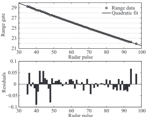
Fig. 8. Upper panel: interpolated range data (open circles) of me-teor 1 and a quadratic fit (solid line). Lower panel: the residuals have a standard deviation of less than 0.03 range gates or about
25 m. In the central part where SNR>15 dB, the standard
devia-tion goes down towards a hundredth of a range gate or about 10 m.
illustrates the cross-correlation with a Doppler shifted but not interpolated version of the transmitted code, which clearly give asymmetric s(r). The bottom panels show the cross-correlation with Doppler shifted interpolated codes. The in-terpolated codes give symmetrics(r).
To compensate for the signal power loss when 16=0, the decoded signal must always be divided by the amplifi-cation of the interpolated code, which differs depending on the value of1. This has been done for the bottom row in Fig. 7 showing decoded signal. In case of1=0, the ampli-fication is 26. The weakest possible ampliampli-fication occurs if
1= ±0.5, and is equal to 19.7 when using this code. With-out compensation, periodic ripples will appear in SNR and RCS profiles of the meteor events. This is the cause of the signature reported by Galindo et al. (2011). We discuss this issue further in Sect. 5.1. The compensation for the loss in signal power outlined above solves the problem of how to differentiate these signatures from actual physical processes, posed by Galindo et al. (2011).
30 40 50 60 70 80 90 100
31 32 33 34 35 36 37 38
IPP
Radial velocity (km/s)
104
105
106
107
IPP
30 40 50 60 70 80 90 100
90 92 94 96 98 100
IPP
Range (km)
Linear fit: 34 553 m/s < vD >: 34 618 m/s
40 50 60 70 80 90
−2 −1 0 1 2 3 4
IPP
X (filled), Y (open) [km] Xstd= 36 m, Ystd = 37 m
30 40 50 60 70 80 90 100
54 55 56
IPP
Meteoroid velocity (km/s)
Radiant with beam steering: az = 122.7 ± 0.1°, ze = 52.4 ± 0.2°
30 40 50 60 70 80 90 100
48° 49° 50° 51° 52° 53° 54°
IPP
Radiant w/o beam steering: az = 122.8 ± 0.1°, ze = 52.3 ± 0.2°
Angle to beam T
signal
(K)
a) b) c)
d) e) f)
30 40 50 60 70 80 90 100−45
−40 −35 −30 −25 −20 −15
RCS (dbsm)
[image:10.595.55.538.66.256.2]Tsignal RCS
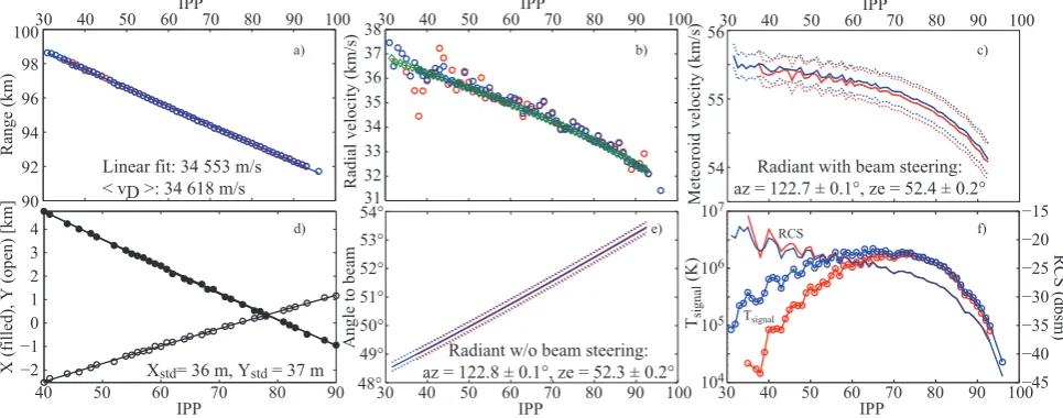
Fig. 9. Overview of the analysis parameters of meteor 1: (a) range, (b) radial velocity, (c) geocentric meteoroid velocity, (d) transversal displacement from beam centre in west and south directions, (e) angle of trajectory to the beam, and (f) RCS and equivalent signal temperature (Tsignal=SNR·Tnoise, whereTnoise'104K). Blue curves represent parameters obtained with, and red curves without, post-beam-steering
throughout all panels. The green markers in (b) trace the velocity determined from pulse-to-pulse phase correlation, presented in greater detail in Figs. 10 and 11. The dotted lines in panels (c) and (e) show the estimated 95 % CI of the meteoroid velocity uncertainty margin and the angle to the beam, respectively.
5.1 The effect of signal processing on BPSK meteor head echo data
When using a 13-bit Barker code oversampled by a factor of 2, as given in Eq. (3), the worst loss of signal due to the cancelling of bauds with opposite phase is'25 %, or about −1.2 dB. If the baud length of a 13-bit Barker code instead is equal to the length of each sample, i.e. if no oversampling is performed, the loss is up to 50 %,or−3 dB.
Our initial analysis of MU meteor head echoes, before we developed this interpolation, resulted in ripples that were identical to those found in JRO head echo observations by Galindo et al. (2011), except for a difference in ripple ampli-tude due to our oversampling. Galindo et al. describe “a peculiar signature present in SNR plots from meteor-head radar returns”. They explain that the signature has “...the following features: (1) strong correlation among fluctuations in SNR values and change in range of a meteor echo, and (2) the fluctuations exhibit periodic ripples with amplitude of 3 dB”. Galindo et al. conclude that “...the understand-ing of this feature is critical to differentiate them from actual physical processes present in meteor returns. Failing to do so could lead to misinterpretation of meteor data.”
It is apparent from Fig. 1a and c in Galindo et al. (2011) that the systematic drop in SNR appears when the leading edge of the echo is in the middle of two range gates, i.e. when
1' ±0.5. An additional investigation of the JRO decoded signal should show that it becomes asymmetric at the same time as SNR drops, in the manner we described for MU data in Sect. 5 and exemplified in Fig. 7.
Galindo et al. (2011) suggest that a possible solution to avoid ripples is increasing the sampling rate with a factor of ∼60 above the transmitter subpulse rate, or from 1 to 60 MHz using their configuration (Chau et al., 2007, Table 1). Know-ing the cause of the ripples enables a simple simulation, where we find that this would decrease the amplitude of the ripples to−0.04 dB. This shows that increasing the sampling rate indeed leads to a satisfactory result. However, the in-terpolation scheme outlined in this paper offers a “cheap” alternative to highly increased sampling, and is in any case advantageous to implement as a complement. It also pro-vides a way to remedy the signal processing issues in already existing data.
The EISCAT meteor code described by Wannberg et al. (2008) and Kero et al. (2008a) is a 32-bit BPSK-coded se-quence oversampled by a factor of 4 at reception. Our sim-ulations show that ripples with an amplitude of '13 %, or −0.6 dB should be present in the data. However, the rip-ple amplitude is small compared to other SNR fluctuations caused by, e.g. fragmentation, quasi-continuous disintegra-tion, etc. (Kero et al., 2008b). Also, the short sampling period of 0.6 µs, which corresponds to range gates with a length of∼90 m, makes systematic appearance of these rip-ples rare. This feature has therefore passed unnoticed in the EISCAT UHF observations.
contain other SNR fluctuations that conceal them, e.g. inter-ference from several meteor targets.
6 Exclusion of data points
Due to deceleration and the geometry of the meteoroid tra-jectory, the radial meteoroid velocity component may change more than 10 % over the short time frame of a meteoroid’s at-mospheric interaction process. For this reason our automatic reduction algorithm must test whether the velocity and range values of consecutive echoes are consistent with a single tar-get or not. This is accomplished as follows: each received radar pulse is analysed separately and its best-fitting Doppler shift, interpolated range gate, signal power and phase, as well as azimuth and elevation angle to the radar target (Sect. 8) are stored as one row in a matrix hereafter called the event ma-trix. An iterative process performs linear least-squares fits on both range versus time and Doppler shift versus time. Resid-ual values more than three standard deviations from either linear fit are excluded from the event matrix and the pro-cedure repeated until there are no more such outliers. De-viating values in either best-fitting velocity, range, or both, caused by simultaneous signals other than the meteor head echo, e.g. echoes from an overdense and enduring meteor trail in a sidelobe, or volume scatter caused by mesospheric turbulence (Reid et al., 1989), or due to an enhanced noise level are thereby excluded. This also provides limits for the temporal extent of the event without having to specify a SNR threshold.
To be able to exclude false rows of data from the initial event matrix but keep those representative of the meteor, we first search for an initial set of data that is likely to represent the meteor. This is accomplished by computing the differ-ence in range and velocity of consecutive rows. As range and velocity in case of a meteor event are estimates of continuous properties, for a row to be classified as representative we re-strict the range values of neighbouring rows to be within one range gate and the Doppler velocity not to differ more than ±3 km s−1. Linear least squares fits are performed on the selected range-time and velocity-time data. Next, the event matrix and these first least-squares fits are exhibited to an it-erative procedure which excludes all rows with range values outside three residual standard deviations of the range-time fit, and velocity values outside ±3 km s−1 of the velocity-time fit. The rows remaining after exclusion of outliers are subject to new linear least-squares fits. Range and velocity is again compared to the respective fit and the procedure re-peated until no further rows can be excluded.
It is expected that different pulse lengths give different best velocity limits. The velocity limit of±3 km s−1 is empiri-cally chosen with respect to the random spread of the Dopp-ler data with the described MU radar experimental setup, and deviation of the meteoroid radial velocity from a linear fit of radial velocity due to its non-linear deceleration.
30 40 50 60 70 80 90 100
−4 −2 0 2 4
Φ (rad)
−10 0 10
−ΔΦ (rad)
30 40 50 60 70 80 90 100
−30 −20 −10 0 10
unwrapped −ΔΦ (rad)
[image:11.595.312.544.61.226.2]Radar pulse
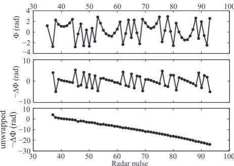
Fig. 10. From top to bottom: phase values (8), phase difference
of consecutive radar pulses (18), and unwrapped phase difference,
all versus radar pulse number of meteor 1.
The data points remaining after exclusion all have SNR exceeding about−3 dB, which may therefore be regarded as the detectability threshold of the analysis.
7 Pulse-to-pulse phase correlation
The fraction of a wavelength a target has moved during two adjacent transmissions can most often be determined very precisely by using pulse-to-pulse phase correlation. The main advantage of doing this is the possibility to determine the shape of the meteoroid velocity curve as a function of time (or altitude). This is necessary for dynamical meteoroid mass and atmospheric entry velocity estimations.
The peak of the convolution of the Doppler-shifted version of the transmitted code with the received signal containing a meteor echo (described in Sect. 5) is a complex number. Its magnitude provides an estimate of the echo power, ampli-fied from the SNR of each sample by a factor of 19.7–26, or 12.9–14.1 dB, depending on the offset (1) between target and sampling.
The phase (8) of the complex number is an estimate of the phase difference between the echo and the Doppler-shifted code. When the same phase is used as reference for analysing consecutive IPPs, their phase difference (18) can be used to estimate how large fraction of a wavelength the target has moved during the IPP. A meteor head echo target will usu-ally have moved several wavelengths when the IPP is of the order of 1 ms and the radar frequency is in the VHF band or higher (>30 MHz). Any integer number of wavelengths for which the target has moved cannot be revealed by pulse-to-pulse phase correlation. The velocity from the phase is there-fore ambiguous with possible solutions separated according to Eq. (1).
30 40 50 60 70 80 90 100 30
31 32 33 34 35 36 37 38
Radar pulse
V
radial [image:12.595.50.285.62.233.2](km/s)
Fig. 11. Unwrapped phase difference (filled circles) and single-pulse Doppler data (open circles) of meteor 1. The integer number of wavelengths to add to the unwrapped phase difference to find
the velocity from the phase isp=36 (blue circles), determined
from comparison with Doppler data. The solid line is a linear least-squares fit to the Doppler data.
Fig. 10. The middle panel shows the difference in phase (18) found by comparing consecutive IPPs. The bottom panel presents an unwrapped version of the phase difference. The unwrap procedure is a search for a smooth phase curve by adding or subtracting integer values of 2π to each value of18shown in the middle panel. In Fig. 11 the calculated phase curve is converted to radial velocity according to
v8,a=
−18 2π +p
λ
2Tipp
, (8)
wherepis an arbitrary integer value,λis the wavelength and
Tippthe length of an IPP.
The correct (or at least the most probable) value ofp is found by comparing the data points of the velocity from the phase (filled circles) with the Doppler velocity data points (open circles) in Fig. 11. For meteor 1 the value isp=36. If the comparison of ambiguous phase data with Doppler data does not provide a clear distinction, range rate data can be used as a second alternative. The quality of the Doppler data in our analysis procedure is generally always good enough to give a clear distinction when a filtering procedure is used. The solid line in Fig. 11 is a linear least-squares fit to the Doppler velocity implemented for this purpose.
An example of an event with less precise Doppler data than meteor 1 is given in Fig. 12. This meteoroid’s initial velocity and deceleration is not possible to determine accurately using the Doppler data alone. However, the Doppler data is good enough to discriminate which of the ambiguous but very pre-cise sets of velocity from the phase that is the most likely one. The velocity determined from the phase reveals how the meteoroid’s deceleration increases during the detection and enables dynamical modelling of it’s mass loss.
220 230 240 250 260 270 280 290 300 310 50
52 54 56 58 60
Radar pulse
V
radial [image:12.595.308.544.64.236.2](km/s)
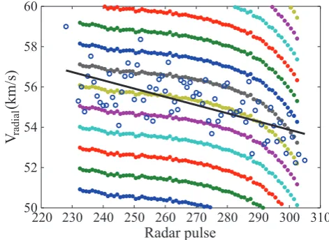
Fig. 12. Unwrapped phase difference (filled circles) and single-pulse Doppler data (open circles) of a meteor detected 28 July 2009, 05:33:08 JST. The integer number of wavelengths to add to the
un-wrapped phase difference is in this casep=55 (yellow circles).
The standard deviation of the velocity determined from the phase as compared to a smooth curve (for this particular example a fourth
degree polynomial gives quite random residuals) is 46 m s−1. The
standard deviation of the Doppler data is about 1 km s−1.
Transmitting radar pulses with unequal IPPs would pro-vide a robust way of unambiguously determining the velocity from phase-to-phase pulse correlation.
7.1 Complications in the calculations
A complication that has to be taken into account in order to acquire an accurate velocity from the phase is that the tar-get will generally travel through several range gates. The fastest targets we detect have a radial velocity of aboutVr=
70 km s−1. They traverse a range gate inRs/Vr'13 ms, that
is one every fourth IPP. Each time the leading edge of the echo appears in a different range gate than previously, the phase difference18will not provide a correct velocity esti-mate, but an estimate that is biased by how much the phase changed during one or several sampling periods, depending on how many range gates the target crossed. We have chosen to compensate for this as follows: each IPP is analyzed in-dependently as described in previous sections. To compare a phase value of an echo in IPP=i, where the echo appeared in range gatesktok+26, with a subsequent echo in IPP=i+1 and range gatesl tol+26, we need to estimate how much the phase has changed in the time(l−k)Ts.
To do this we use the average Doppler shift (f¯
D) from the
single-pulse analysis according to
δ8=Ts(l−k)2πf¯D, (9)
whereTs is the sampling period. The value ofδ8is added
For targets with a radial velocity of, e.g.Vr=70 km s−1,
the Doppler shift isfD'2f0Vr/c0'21.7 kHz when using
an operating frequency off0=46.5 MHz. The phase
com-pensation is in this caseδ8'0.82 rad or about 0.13λwhen the target passed from one range gate to another (l−k=1).
For long-duration meteors with large total decelerations, the velocity at any given instant of time may differ from the average velocity by up to about±5 km s−1. Such a velocity difference equals a Doppler shift difference from the average of±1.5 kHz at 46.5 MHz operating frequency.
The phase error (δ8error) introduced by using f¯D may
therefore be up to about
δ8error'1500·2π Ts'0.06 rad, (10)
thus less than 0.01λ. This is equivalent to introducing a ve-locity error of
Verror=δ8errorλ/(2π 2Ts)'10 m s−1 (11)
for this particular velocity estimate. An error of the order of
Verror'10 m s−1 is comparable to or smaller than the
stan-dard deviation of the data points of the velocity from the phase (as compared to a smooth curve). Thus, it is small enough not to tamper with further calculations. However, when the final radial velocity is estimated as a function of time, these data points can be recalculated to decrease errors if necessary.
8 Interferometry
Interferometry calculations are performed on all rows of the original event matrix before the exclusion of data described in Sect. 6. We have for this purpose implemented the mul-tiple emitter location and signal parameter estimation (MU-SIC) method developed by Schmidt (1986). It is based on a signal subspace approach suitable for point sources and where the data can be described by an additive noise model (Schmidt and Franks, 1986). Radar studies of meteor head echoes fulfill these criteria. MUSIC, therefore, allows rapid and precise estimations of the signal direction of arrival (DOA). When the criteria are fulfilled, Schmidt (1986) shows that MUSIC can be used to find asymptotically unbiased es-timates of, e.g. the number of signals and their DOA for up toK < Mmultiple source directions, whereMin the case of the MU radar is the number of subarraysM=25.
A comparison of MUSIC with other methods as ordinary beamforming, maximum likelihood and maximum entropy is given by Schmidt (1986).
Guided by Manikas et al. (2001), we have defined an an-tenna manifold vectorϒ(θ,φ)as
ϒ(θ,φ)=γ(θ,φ)exp(−jrTk), (12) whereθ is the azimuth (measured positive east of north),
φ is the elevation, r= [rx,ry,rz]T ∈R3×M are the an-tenna subgroup centre locations with respect to the
geo-metric centre of the whole array expressed in radar wave-lengths (and subgroup F5 is located at [0,0,0]), k= 2π[cosφsinθ,cosφcosθ,sinφ]T∈R3×1is the wavenumber vector, is the Hadamard product (elementwise multipli-cation of the matrices) andγ(θ,φ)∈CM×1is a vector con-taining the directional gains of the subgroups. The one-way half power beam width of a single antenna subgroup is 18◦. We have in the calculations used unity directional gain for all subgroups, which works well for the purpose of direc-tion finding of targets close to zenith. Furthermore, the MU radar antenna field being horizontally aligned givesrz=0
and means that Eq. (12) can be simplified as
ϒ(θ,φ)'exp(−2πj (rxcosφsinθ+rycosφcosθ )). (13)
The displacementsrxandryof the subgroup centres are
il-lustrated in Fig. 2.
The MUSIC spectrum is calculated as MUSIC(θ,φ)= ϒ(θ,φ)
0ϒ(θ,φ)
ϒ(θ,φ)0Q
nQ0nϒ(θ,φ)
, (14)
where Qn contain the noise eigenvectors. We estimate Qn
by first computing a spatial covariance matrix R from the
M=25 set of complex voltages, one from each receiver channel, and each one containing the N=27 samples se-lected as containing the meteor echo (as described in Sect. 5), according to R=XX0/N, where X is aM×N matrix con-taining the received data. An eigendecomposition of the co-variance matrix,[Q,D] =eig(R), gives a set of eigenvectors Q and associated eigenvaluesD.
Each present source gives rise to a distinct nonzero eigen-valueDK. If the noise would be zero, there would only be as many nonzero eigenvalues as there are sources (Schmidt and Franks, 1986). Unfortunately noise is seldom zero in an experimental system. Source eigenvalues and noise eigen-values must therefore be told apart, the former have larger magnitudes.
In our present implementation we are only searching for one point target. We assume that this target gives rise to the largest eigenvalueDmaxamongDand that its associated
complex vectorQmaxtherefore defines the signal subspace.
The exclusion of Qmax and orthogonality of eigenvectors
means that the remaining eigenvectors Qn(i.e. all
eigenvec-tors of Q except the one associated withQmax) now spans
the orthogonal complement of the signal subspace, perhaps most appropriately called the signal nullspace (Schmidt and Franks, 1986). When evaluating Eq. (14) for different DOA, the denominator will approach zero in the vicinity of the sig-nal DOA and there cause a narrow peak in the spectrum.
υ1
Transmitter/Receiver
υ2
[image:14.595.66.269.62.259.2]Meteoroid trajectory
Fig. 13. Exaggerated sketch of a meteoroid trajectory in the far-field of a radar beam (solid lines), where the phase fronts are spherical
(dashed lines). The Doppler shift varies as cosυalong the trajectory.
For an approaching meteoroid the angleυ1< υ2, which leads to a
decreasing radial velocity component.
and the DOA finally searched for within a small fraction of a degree. Each determined DOA is then stored in the event matrix to enable trajectory estimation.
9 From line-of-sight to vector velocity
It is very important to carefully take the geometrical consid-erations into account when estimating a meteoroid’s velocity from measured radial quantities. This may sound as a su-perfluous comment, but underestimated flight parameter un-certainties may perhaps explain the anomalous acceleration reported by, e.g. ˇSimek et al. (1997) and Close (2004). Fig-ure 13 shows an exaggerated sketch of a meteoroid trajectory in the far-field of a radar beam. The angle between the tra-jectory and the beam isυ, and the radial component of the velocity vector varies as cosυ. Kero et al. (2008a) showed that this gives rise to an apparent acceleration/deceleration term (depending on if the meteoroid is approaching or reced-ing from the radar) that is of the same order of magnitude (and often larger) than the true meteoroid deceleration.
To calculate the meteoroid trajectory, we begin by search-ing for and includsearch-ing as many successful interferometry data points as possible from each meteor. We start by assuming that the detected trajectory is straight, i.e. the curvature of the trajectory (due to Earth gravity) within the radar beam is negligible.
Azimuth and elevation depend non-linearly on position along a straight trajectory. Therefore, we do all calculations in a Cartesian coordinate system; its origin located at the cen-tre of the MU radar, the x-axis pointing east, the y-axis north
South
West
[image:14.595.337.520.63.249.2]85º 86º 87º 88º 89º
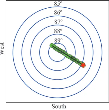
Fig. 14. Top view of the set of instantaneous target locations at each IPP (green circles) of meteor 1, the start of the event (red star) and a fit of the trajectory (black line). The contours of constant elevation,
85◦to 90◦, (blue) correspond to radial distances of about 1.7 km at
100 km range.
and the z-axis completing the set by pointing towards local zenith. Figure 14 shows a top view of the set of DOA of me-teor 1 (green circles). The event starts at the red star and a fit of the trajectory is drawn as a black line.
Occasionally, plasma in the trail left behind the meteor-oid may constitute a target and interfere with the head echo position determination. To exclude these targets we fit both cartesian coordinatesx andy versus time and exclude out-liers rather than fittingy versusx. Such plots of meteor 1 is displayed in Fig. 9d.
We are ultimately interested in finding not only the az-imuth of the radiant but also its zenith distance. For this reason, we estimate and compare the meteoroid’s transver-sal velocity component obtained from interferometry to its radial velocity component. We proceed as follows.
First we make a linear fit ofx versus time andy versus time, using the remaining data points after the iterative pro-cedure described in Sect. 6. Then we continue to exclude outliers (data points more than three standard deviation from any of the fits) in a iterative routine until no more points can be excluded.
We assume that the linear fits give reasonable estimates of the transversal velocity components at the central point (pc)
of the detection. For meteor 1, the radar pulsepc=64 is the
central point of the event. Thus, the slopes of the linear fits ofx andy give us velocity componentsvx(pc)andvy(pc).
If the values of these linear fits atpcare calledX(pc)and
Y (pc), they can together with the very precise range data
of the same instant, r(pc), be used to define a most
prob-able meteoroid position Pxyz(pc)= [X(pc),Y (pc),Z(pc)],
whereZ(pc)=
p
The radial velocity component at the same instant (pc) is
best described by the velocity found using the phase correla-tion method explained in Sect. 7. We use it to estimate the vertical velocity componentvz(pc)according to
vz(pc)= (15)
vradial(pc)−cosφ (pc)(vy(pc)cosθ (pc)+vx(pc)sinθ (pc))
sinφ (pc)
,
whereθ (pc)andφ (pc)are the azimuth and elevation angles
to the location of the target atpcas measured from the
sym-metry axis of the radar. The radiant of the meteor (i.e. the direction from which the meteoroid appears to originate) is expressed in terms of a different set of angles, the azimuth
azradiantand the zenith distancezdradiant. These are in
hori-zontal coordinates found by
azradiant=π+arctan(vx(pc)/vy(pc)), (16)
whereazradiantis measured east of north, i.e. towardsxfrom
y) and arctan computes the arctangent within a range of [−π,+π], and
zdradiant=
π
2 −arctan
−vz(pc)/
q
vx(pc)2+vy(pc)2
,(17) where zdradiant is zero for a meteoroid originating from
zenith.
Computing the velocity curve containing also the deceler-ation is more difficult than making a single vectorial velocity estimate. The trickiest part is converting the accurate radial meteoroid velocity to a reasonably accurate velocity along the trajectory. The reason is that the instantaneous position of the meteoroid (as well as a fit to the position data) has much lower precision than the radial velocity has. Further-more, the error introduced by assuming, e.g. that the angle to the beam increases linearly (Chau and Woodman, 2004) leads in some cases to an acceleration at the beginning of the event and too fast deceleration at the end, compared to the true values, and in some cases to errors of opposite signs.
To circumvent these problems we use neither a linear as-sumption on the target angular velocity nor the instantaneous position of the target as a function of time found from in-terferometry and range, but propagate the target along the determined trajectory (assuming only it is straight) applying the radial velocity itself. For this we only need to use the al-ready defined positionPxyz(pc)and the radiant. If the radial
velocity atpcisvradial(pc)then the meteoroid velocity at that
point is
vmet(pc)=
vradial(pc)
cosα(pc)
, (18)
where the angle between the trajectory and the line-of-sight vector from the radar to the target isα(pc). This angle is
given by
α(pc)=π−arccos
Pxyz·vxyz
|Pxyz·vxyz|
, (19)
where vxyz is the meteoroid velocity vector. As we have
assumed that the trajectory is straight, only the magnitude
vmet=|vxyz|of the velocity vector changes whereas the
di-rectionbvxyz= vxyz
|vxyz| remains the same throughout the
calcu-lations.
The estimatedvmet(pc)can now be used to propagate the
meteoroid along the trajectory. Its locationPxyz at an
adja-cent time of determined radial velocity is found by multiply-ingvmet(pc)with the time intervalδt(whereδt=Tippif there
is a velocity estimate available from the closest possible pair of received radar pulses) and therefore equal to
Pxyz(pc+1)=Pxyz(pc)+vmet(pc)bvxyzδt. (20)
The new position can be used to readily evaluate the new meteoroid velocity from the adjacent radial velocity estimate. We use Eqs. (18) through (20) in an iterative procedure in both directions from the central point (pc) and thus employ
the full precision of the estimated radial velocity to find the meteoroid velocity curve, permitting deceleration and initial velocity to be deduced as accurately as possible.
9.1 Error estimation
The largest error in the velocity curve is introduced by the uncertainty of the angle between the trajectory and the beam. To evaluate how this uncertainty affects the velocity curve we estimate confidence intervals (CI) for the linear fit co-efficients of the interferometric data. Simultaneously, this also gives us radiant uncertainty regions. The CI are con-structed by calculating the standard errors of the ordinary least squares solutions and multiplying them with the 95 % parameter of the studenttdistribution (e.g. Hamilton, 1992). Using so determined CI for both zenith distance and az-imuth we construct an elliptical area (circular if the uncer-tainties in both directions are equal), which contains the true meteoroid radiant with 95 % certainty under the condi-tion that the residuals of the interferometry data are random and normally distributed. To find boundaries for the veloc-ity curve we apply the iterative process described above but withbvxyz of Eq. (20) replaced by vectors corresponding to
the smallest and largest angle to the beam within the radiant area. Meteoroid velocity curves for meteor 1 computed in this manner are plotted as dotted lines in Fig. 9c. Its initial velocity is 55.5±0.2 km s−1 and the deceleration does not change significantly within the estimated uncertainty region. Because a meteoroid’s initial deceleration can be very small, an error as little as of the order of 1◦ can indeed
60 80 100 120 140 160 180 78°
80° 82° 84° 86° 88°
IPP 60 80 100 120 140 160 180
94.5 95.0 95.5 96.0 96.5
IPP
Range (km)
60 80 100 120 140 160 180
0 1 2 3 4 5 6 7 8
IPP
Radial velocity (km/s)
60 80 100 120 140 160 180 −3
−2 −1 0 1 2 3
IPP
X (filled), Y (open) [km]
60 80 100 120 140 160 180
25 30 35 40
IPP
Meteoroid velocity (km/s)
Angle to beam
60 80 100 120 140 160 180 IPP
104 105 106
Tsignal
(K)
−36 −35 −34 −33 −32 −31 −30 −29
RCS (dbsm)
Linear fit: 3 635 m/s < vD >: 3 894 m/s
Xstd= 112 m, Ystd = 79 m
Radiant with beam steering: az = 38.3 ± 0.9°, ze = 82.7 ± 0.3°
Radiant w/o beam steering: az = 37.7 ± 0.7°, ze = 82.7 ± 0.4°
a) b) c)
d) e) Tsignal f)
[image:16.595.50.548.67.254.2]RCS
Fig. 15. Overview a meteor detected 14 December 2010, 00:01:29 JST: (a) range, (b) radial velocity, (c) geocentric meteoroid velocity, (d) transversal displacement from beam centre in west and south directions, (e) angle of trajectory to the beam, and (f) RCS and equivalent
signal temperature (Tsignal=SNR·Tnoise, whereTnoise'104K). Blue curves represent parameters obtained with, and red curves without,
post-beam-steering throughout all panels. The green markers in (b) trace the velocity determined from pulse-to-pulse phase correlation, presented in greater detail in Fig. 11. The dotted lines in panels (c) and (e) show the estimated 95 % CI of the meteoroid velocity uncertainty margin and the angle to the beam, respectively.
to 29.2±1 km s−1. In fact, it can be limited even further, to 28.6±0.4 km s−1, if deceleration is presumed.
The closer a meteoroid trajectory is to perpendicular to the beam, the more sensitive is the deceleration determination to errors. However, as the deceleration initially can be very small, an overestimated angle to the beam may cause mete-oroids on all slant angles to appear to be accelerating. Con-versely, if the angle to the beam is underestimated, a meteor-oid will appear to decelerate faster than it does. The latter is an error less likely to be noticed, as meteoroids are expected to decelerate. Nevertheless, mass calculations based on the standard momentum equation (Bronshten, 1983, p. 12), us-ing the velocity (v) and deceleration (v˙) obtained from an event which angle to the beam is underestimated will result in an underestimated meteoroid mass. When the cross-sectional area of the meteoroid is rewritten using an arbitrarily chosen meteoroid shape factor (Bronshten, 1983, p. 14), it is easily seen that meteoroid mass is proportional tov6/v˙3 (Campbell-Brown and Koschny, 2004, Sect. 2.4 and Eq. 2). Small errors invandv˙, therefore, quickly cause large errors in estimated mass (Kero et al., 2008a).
10 Radar cross section
Radar cross sections (RCS) of detected targets are evaluated by rewriting the classical radar equation (e.g. Skolnik, 1962) as
RCS= (4π )
3P rR4
Gr(θ,φ) Gt(θ,φ) λ2Pt
, (21)
where
Pr= received power,
R = target range,
Gt= transmitter antenna gain,
Gr= receiver antenna gain,
θ = azimuth of target (positive east of north),
φ = elevation of target,
λ = radar wavelength, and
Pt= transmitted power.
The received power is given by
Pr=SNR·TnoisekBbw, (22)
where SNR is the signal-to-noise ratio,Tnoise is the
equiv-alent noise temperature, kB=1.38×10⁻²³J K−1 is the
Stefan-Boltzmann constant, and bw'1/6 µs≈167 kHz is
the receiver bandwidth. Tnoise=Tsys+Tcosmicis the sum of
the system noise (Tsys∼3000 K) and the cosmic background
radio noise that varies from aboutTcosmic∼5000–15 000 K
throughout one diurnal cycle. Tcosmic is dominated by the
passage of two strong radio sources close to zenith, Taurus-A and Cygnus-Taurus-A. Except for the receiver noise temperature and noise contribution due to losses in feed,Tsysmay in this
context also include contribution from atmospheric emission and ground radiation (spillover and scattering). To proceed, we assume thatTsysis constant throughout each diurnal
cy-cle. This is not necessarily true, but as long as bothTsysand
its variance are small with respect toTcosmic, the assumption