www.biogeosciences.net/11/1199/2014/ doi:10.5194/bg-11-1199-2014
© Author(s) 2014. CC Attribution 3.0 License.
Biogeosciences
Can the heterogeneity in stream dissolved organic carbon be
explained by contributing landscape elements?
A. M. Ågren1, I. Buffam2, D. M. Cooper3, T. Tiwari1, C. D. Evans3, and H. Laudon1
1Department of Forest Ecology and Management, Swedish University of Agricultural Sciences, S901 83, Umeå, Sweden 2Department of Biological Sciences and Department of Geography, University of Cincinnati, 312 College Drive, Cincinnati,
OH 45221, Ohio, USA
3Centre for Ecology and Hydrology, Deiniol Road, Bangor, LL57 2UP, UK
Correspondence to: A. M. Ågren ([email protected])
Received: 16 September 2013 – Published in Biogeosciences Discuss.: 15 October 2013 Revised: 21 January 2014 – Accepted: 26 January 2014 – Published: 27 February 2014
Abstract. The controls on stream dissolved organic carbon (DOC) concentrations were investigated in a 68 km2 catch-ment by applying a landscape-mixing model to test if down-stream concentrations could be predicted from contribut-ing landscape elements. The landscape-mixcontribut-ing model repro-duced the DOC concentration well throughout the stream network during times of high and intermediate discharge. The landscape-mixing model approach is conceptually sim-ple and easy to apply, requiring relatively few field measure-ments and minimal parameterisation. Our interpretation is that the higher degree of hydrological connectivity during high flows, combined with shorter stream residence times, in-creased the predictive power of this whole watershed-based mixing model. The model was also useful for providing a baseline for residual analysis, which highlighted areas for further conceptual model development. The residual anal-ysis indicated areas of the stream network that were not well represented by simple mixing of headwaters, as well as flow conditions during which simple mixing based on head-water head-watershed characteristics did not apply. Specifically, we found that during periods of baseflow the larger valley streams had much lower DOC concentrations than would be predicted by simple mixing. Longer stream residence times during baseflow and changing hydrological flow paths were suggested as potential reasons for this pattern. This study highlights how a simple landscape-mixing model can be used for predictions as well as providing a baseline for residual analysis, which suggest potential mechanisms to be further explored using more focused field and process-based mod-elling studies.
1 Introduction
Dissolved organic carbon (DOC) is a key constituent in sur-face waters as it has fundamental implications for the ecology and biogeochemistry of aquatic ecosystems. The important role of stream DOC has resulted in several recent investiga-tions to better understand the mechanisms of DOC regula-tion across temporal and spatial scales (Tank et al., 2012; Temnerud and Bishop, 2005). A general finding has been that the variability of stream DOC concentrations within and between adjacent streams can be as large as the variability found on a regional or even global scale (Bishop et al., 2008). Although much of this variability can be explained by the occurrence of organic soils in the catchments (Creed et al., 2003; Walker et al., 2012), peatlands alone do not explain the large spatial heterogeneity of DOC in the landscape (Matts-son et al., 2009; Ågren et al., 2007).
Tank et al., 2012). While the accumulation of organic matter in unforested mires makes them the major source of DOC in the boreal landscape (Rantakari et al., 2010; Ågren et al., 2007), forested areas, which generally have the greatest areal extent in the boreal biome, also contribute large DOC con-centrations because of the presence of organic-rich riparian soils (Grabs et al., 2012; Knorr, 2013).
The relative proportion of mires and forest in the land-scape can be used as a first-order approximation to predict the stream DOC concentration in small streams (Aitkenhead et al., 1999; Laudon et al., 2012). However, as the catchment size increases from headwaters to meso-scale catchments, so does the complexity of the contributing factors controlling stream water chemistry (Bloschl and Sivapalan, 1995). This increased complexity can be related to new/different con-tributing landscape features becoming increasingly common downstream at lower elevations, but also because there may be scale-dependent processes that can have considerable ef-fects on the stream DOC concentrations as the rivers grow, for example changing flow paths (Cey et al., 1998) or effects of landscape structure (Pacific et al., 2010).
Another characteristic feature of DOC is the large tem-poral variability related to hydrological events, seasonal dif-ferences and inter-annual conditions (Dawson et al., 2011). Hydrology has a first-order control on DOC concentrations in individual catchments (Hinton et al., 1997; Laudon et al., 2011; Raymond and Saiers, 2010). Drying and re-wetting of catchment soils (Köhler et al., 2008), soil temperature (D’Amore et al., 2010), winter climatic conditions (Haei et al., 2010) and antecedent conditions controlling the pool of sorbed, potentially soluble organic carbon (Ågren et al., 2010; Yurova et al., 2008) can affect DOC concentrations on an event, seasonal and annual timescale. This temporal vari-ability adds to the spatial complexity of DOC concentrations, as different catchment characteristics can differ in response to hydrological and climatic forcing depending on catchment soils, vegetation and topography. Furthermore, depending on the spatial configuration of the landscape, the residence time of water in the surface water network can moderate or exag-gerate the response in downstream locations in ways that are not easily predictable.
Because of the large complexity of factors controlling stream DOC concentrations we tested a simple conceptual landscape-mixing model as a predictive and diagnostic tool on a large nested boreal stream data set, to better under-stand how DOC is regulated during different seasons and across scales. The main objectives of this study were (1) to test if the spatial heterogeneity of stream DOC concentra-tions can be explained by the major contributing landscape elements; and (2) to use a residual analysis as a diagnostic tool and a learning framework for further development of our conceptual understanding. To answer these questions we used a landscape-mixing model on the 68 km2boreal Kryck-lan catchment. A Kryck-landscape-mixing model (Cooper et al., 2004; Cooper et al., 2000; Evans et al., 2001) offers a
sim-ple approach to modelling stream biogeochemistry by lump-ing processes into dominatlump-ing landscape elements that can be used to examine if the DOC concentration is simply due to the conservative mixing of contributing sources. Firstly, we investigate how the landscape-mixing could be used to predict DOC, using several model assessment criteria. Sec-ondly, we analyse the model residuals to investigate model performance and thereby answer the question of where in the landscape simple mixing of stream water does not adequately characterise stream DOC behaviour. By running and validat-ing the model on data sampled on seven different occasions, we also addressed the question of whether the landscape-mixing model performed better at certain times of the year, or under certain flow conditions. Using this simple concep-tual approach the ultimate goal was to provide new insights into the mechanisms regulating stream DOC and how these may vary across a landscape and during different times of the year.
2 Materials and methods
2.1 Study catchment
The 68 km2 Krycklan catchment (64◦160N, 19◦460E) was used as a study catchment for modelling the spatial variabil-ity of DOC in the stream network (Laudon et al., 2013). The Kryklan catchment is a glaciated forested catchment (forest cover 87 % and peatland cover 9 %). The forest is dominated by Scots pine (Pinus sylvestris) and Norway spruce (Picea
abies) with an understorey dominated by ericaceous shrubs,
mostly bilberry (Vaccinium myrtillus) and lingonberry
(Vac-cinium vitis-idaea) on moss mats of Hylocomium splendens
and Pleurozium schreberi (Forsum et al., 2008). Quater-nary deposits of till, peat and fine sorted sediments are the dominant overburden (Fig. 1). The peatlands are classified as forested (2/3) or open (1/3). The peat is dominated by
Sphagnum species and consists of mostly minerogenic, acid
Fig. 1. Map showing the Quaternary deposits for the catchment. The
aggregation of the surficial geology cover into groups is indicated in the legend (letters A–D) according to the regression model used to estimate DOC concentrations. Superimposed on the map is a layer showing the modelled DOC concentrations (September 2008) for every 5 m section of the stream network. The white dots indicate the 115 sampling sites.
1.8◦C and the annual precipitation is 640 mm, of which ap-proximately half enters streams as runoff (Oni et al., 2013).
2.2 Stream water sampling
Stream water was sampled at 115 sites throughout the catch-ment on seven occasions from May 2003 to Sept 2008 dur-ing different seasons and hydrological conditions (Table 1 and Fig. 2). The sampling campaigns were designed to take a “snapshot” of the spatial variability of the stream network, and on each occasion, sites were sampled during a single day, except during winter baseflow, where sampling extended over a week. While 115 different site locations were sampled in total, the number of sites sampled in any particular survey varied between 73 to 89. A subset of 42 sites was sampled on all seven occasions.
Discharge was measured in a second-order stream in the central area of the catchment (called Svartberget or C7 in previous studies; Laudon et al., 2007) at a 90◦ V-notch weir located inside heated housing. Pressure transducers con-nected to Campbell scientific data loggers, USA or dupli-cate WT-HR capacitive water stage loggers, Trutrack Inc., New Zealand were used to record the water level. Using established rating curves the water stage was used to cal-culate discharge. We make the simplifying assumption that the specific discharge is the same throughout the catchment.
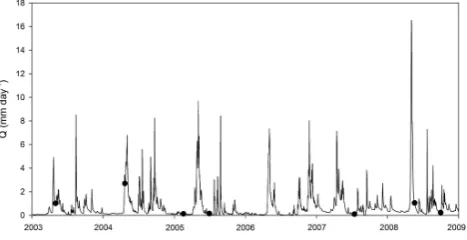
Fig. 2. The variability in discharge for 2003–2008; the black dots
indicate the dates for the 7 sampling occasions.
The uncertainty this assumption introduces has been calcu-lated to be on average at most 12 % (Ågren et al., 2007), but can be higher under particularly low flow conditions (Lyon et al., 2012). The water samples were collected in acid-washed and sample-rinsed high density polyethylene (HDPE) bottles (Embalator Mellerudplast, Mellerud, Swe-den) and were stored frozen until they were analysed for DOC using a Shimadzu TOC-VCPH/CPN analyser (Shi-madzu, Kyoto, Japan).
2.3 Watershed characteristics
Lidar (Light detection and Ranging) measurements of the catchment have been made at a point density of 3.3–10.2 measurements per m2. These data were used to generate a 0.5 m high-resolution DEM. For hydrological modelling the DEM was aggregated to a 5 m resolution. In order to make the DEM flow compatible it was manually corrected where bridges and road culverts obstructed the flow algo-rithm, and all sinks were filled. The catchment delineation was then derived automatically from the DEM using ArcGIS 10.0. Care was taken to ensure that the catchment delineation was correct for all 115 catchments, and manual adjustments were made to the DEM in questionable sections based on a 3-D version of the 0.5 m DEM combined with field ob-servations. For each sub-catchment the catchment charac-teristics were derived using map data. DOC was modelled from the surficial geology cover based on the Quaternary de-posits map (1 : 100 000) (Geological Survey of Sweden, Up-psala, Sweden). Additional catchment characteristics were derived for all sub-catchments for potential use as covari-ates in the residual analysis. These characteristics included stream order, catchment area, slope, topographic wetness in-dex (TWIMD8) (Grabs et al., 2009), proportion above the
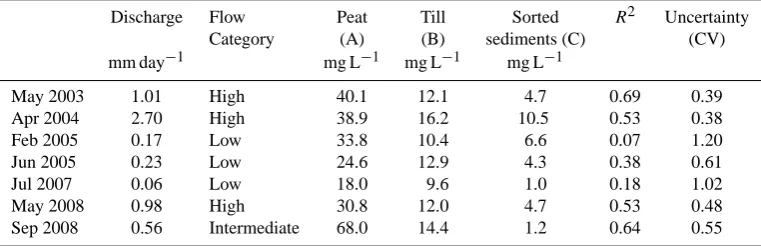
[image:3.595.50.286.67.302.2]Table 1. Discharge (mm day−1)for each sampling occasion and the estimated end-member concentrations (mg L−1)from bootstrapping (n=15).R2is theR2from the bootstrapping procedure (Eq. 1). To the right is the uncertainty in modelled concentrations expressed as the coefficient of variation (CV) from the Monte Carlo analysis.
Discharge Flow Peat Till Sorted R2 Uncertainty Category (A) (B) sediments (C) (CV) mm day−1 mg L−1 mg L−1 mg L−1
May 2003 1.01 High 40.1 12.1 4.7 0.69 0.39
Apr 2004 2.70 High 38.9 16.2 10.5 0.53 0.38
Feb 2005 0.17 Low 33.8 10.4 6.6 0.07 1.20
Jun 2005 0.23 Low 24.6 12.9 4.3 0.38 0.61
Jul 2007 0.06 Low 18.0 9.6 1.0 0.18 1.02
May 2008 0.98 High 30.8 12.0 4.7 0.53 0.48
Sep 2008 0.56 Intermediate 68.0 14.4 1.2 0.64 0.55
Lidar measurements and regression models with field ob-servations, detailed maps were constructed providing, for each 10*10 m pixel, forest stand height, birch (Betula spp) biomass, lodgepole pine (Pinus contorta) biomass, Norway spruce biomass, Scots pine biomass, total biomass and mean forest stand age. Averages of all the forest variables were cal-culated for each sub-catchment.
2.4 End members and landscape-mixing modelling
The landscape-mixing model, which was based on Cooper et al. (2004) and Cooper et al. (2000), predicts water chemistry throughout a stream network from landscape properties. The model is based on the assumption that the variability within a landscape type is smaller than between landscape types, and that different landscape elements generate different so-lute concentrations. These landscape concentrations are esti-mated from sampling data at stream locations draining sub-catchments with known upstream proportions of each land-scape type. A detailed DEM (digital elevation model) with 5 m resolution and the presence of many sampling sites in our study allows us to work with the actual sub-catchments and at a high resolution. We used a statistical approach to calculate the end-member concentrations from the different landscapes. In order to more easily compare model perfor-mance between all seven sampling occasions we selected headwater catchments that were sampled on all occasions as the data set for model parameterisation. Small catchments with more uniform landscape characteristics will tend to have concentrations which are closer to the different end mem-bers and more representative of sources, while larger catch-ments, through mixing of upstream sources, show a reduced variability (Temnerud and Bishop, 2005). We therefore se-lected only catchments with area less than or equal to 3 km2 for model parameterisation. Fifteen catchments fulfilled both criteria (sampled on all occasions, size≤3 km2); the remain-ing samplremain-ing sites were used to assess model performance, particularly to test the simple mixing hypothesis.
Previous research in the catchments has identified three landscape types which are expected to give rise to contrast-ing stream water chemistry, includcontrast-ing DOC concentrations (Ågren et al., 2007; Buffam et al., 2008). We have termed these landscape types “peat”, “till”, and “sorted sediments”, based on the corresponding surficial geology deposits under-lying each landscape. The variation in surficial geology in-fluences other landscape characteristics including weather-ing rates and drainage, which in turn influence soil forma-tion, vegetaforma-tion, subsurface hydrologic flow paths and rates, and riparian zone formation. All of these are expected to in-fluence DOC, thus the surficial geology categories serve as a useful tool for categorisation. From the surficial (Quaternary) geology map each of the 115 catchments was classified by relative proportion of (A) peat, (B) till (this also includes the “thin soil” class which in essence is a shallow layer of till on bedrock), (C) sorted sediments (silt, sand and glaciofluvial alluvium) or (D) “other” (lakes and rock outcrops). Based on the 15 selected headwater sites in the construction data set, a regression model (Eq. 1) was constructed to calculate the end-member concentrations for each landscape type and on each sample date by multiplying the concentration with the areal coverage for each landscape type (A–D). By set-ting the intercept to 0 in the model and using the areal cov-erage of the landscape types in proportions (0–1) instead of percentages, the estimates (A–D) were expressed directly as the end-member concentration for DOC in mg L−1for each landscape type.
[DOC]mg L−1=A×[DOC]Peat+B×[DOC]Till (1)
+C×[DOC]Sorted sediment+D×[DOC]Other
included twice, or more, until the data set again comprised 15 streams. Slopes and constants were calculated for every new data set, then the randomisation process was repeated 1000 times. Finally, mean concentrations were computed for each landscape component and used in the model (Table 1). This method has the additional benefit that it provides an estimate of the uncertainty in the end-member concentra-tions. Based on the repeated runs, the standard errors, con-fidence intervals, and correlations were calculated for each end-member concentration. The uncertainty in the calculated end-member concentrations was later used to analyse the to-tal uncertainty of the models. All bootstrapping calculations were done in PASW Statistics 18 (SPSS Inc.). Initially, the bootstrapping procedure sometimes generated unrealistic es-timates. To overcome this, constraints were set on the end-member concentrations. Soil water data from the catchment were used as constraints for concentrations of each landscape type. For peat, lower and upper limits of 4 and 84 mg L−1
were set, based on measurements from groundwater wells in a wetland in the catchment (Yurova et al., 2008). For till the acceptable range was set to 1–97 mg L−1given the vari-ability in lysimeter measurements from 10 soil profiles in till-derived soils in the catchment (Grabs et al., 2012). In fine sorted sediments the constraint was set to 1–46 mg L−1 given the variability in lysimeter measurements from three soil profiles in the fine sorted sediment-derived soils in the catchment (Grabs et al., 2012). In the first attempt, the end-member concentration for landscape type “other”, consisting of lakes and bare rock (D in Eq. 1), was calculated. The eval-uation showed that the end-member concentration for D was extremely variable and uncertain and including these values did not improve the fit for the overall model. Because of this uncertainty and since class “other” had such a minor areal coverage (on average about 2 % and at maximum below 10 % coverage; Fig. 3), the parameter D in Eq. (1) was set to 0.
2.5 Landscape-mixing modelling in GIS
The high-resolution DEM facilitated modelling of DOC con-centrations every 5 m throughout the entire stream network using the landscape-mixing model and ArcMap 10 hydrolog-ical modelling tools. Using a weighting raster containing the end-member concentrations for the aggregated surficial ge-ology map (aggregated into the four classes) when perform-ing the flow accumulation calculation, the DOC export from each cell was calculated. The DOC export was then divided by estimated discharge to calculate the DOC concentrations for all 5×5 m cells in the landscape. The modelled DOC concentration for the sampling sites could then be extracted. The modelled DOC values were compared to the measured values for the respective site on each sampling occasion. A layer showing the modelled DOC concentrations for every 5 m section of the stream network could also be displayed (Fig. 1).
2.6 Model validation
Model performance was assessed using data from the sites that were not used for model construction. We calculated several measures (Table 2 and Fig. 4). Root mean square er-ror (RMSE) has the benefit that it gives the erer-ror in units of mg L−1. To standardise RMSE we calculated the RMSE-observation standard variation ratio (RSR). A low RSR in-dicates a better model and values below 0.7 are considered a satisfactory model (Moriasi et al., 2007). As a measure of the average tendency of the modelled values to be larger or smaller than observed values, the percent bias (PBIAS) was calculated. For PBIAS the optimum value is 0, negative val-ues indicate a model overestimation bias and positive valval-ues an underestimation of modelled values. We also plotted the measured and modelled values (Fig. 4) and used standard re-gression measures ofR2and slope. A slope near 1 indicates that the model is close to the 1 : 1 line, a large diversion from 1 indicates a systematic error in the model. As an example, a slope below 1 means that high DOC concentrations are un-derestimated and low values are overestimated. TheR2value indicates the strength of the relationship is between the mea-sured and predicted values, but does not take into account any systematic errors in the slope of the relationship. Nash– Sutcliffe efficiency (NSE) indicates how well the scatter fits the 1 : 1 line; the value of NSE is similar toR2in that a value close to 1 indicates a good fit and a value close to 0 indicates a poor fit.
2.7 Uncertainty
One source of uncertainty in the model is the representative-ness of the 15 selected catchments. To test how this affected the modelled DOC, the bootstrapping routine was rerun us-ing all available sites to calculate the end-member concen-trations for the entire data set. The landscape-mixing model was then rerun on new estimates and an evaluation on how that affected RMSE, RSR, PBIAS and NSE was calculated (Table 3).
A second source of uncertainty was related to the end-member concentrations. However, by using the bootstrap-ping method this uncertainty was calculated (Fig. 5). A Monte Carlo analysis was performed to propagate the un-certainties of the end-member concentrations to calculate an overall uncertainty for the modelled values. The overall un-certainty was calculated using 10 000 realisations with ran-dom parameters assuming that the uncertainty in A, B and C was normally distributed. The uncertainty was expressed as a coefficient of variation (standard deviation of the modelled values/average of the modelled values) (Table 1).
2.8 Residual analysis
Fig. 3. Boxplots showing the percent coverage of each landscape type in the construction (n=15) and validation data sets (n=100).
Table 2. Model performance measures for the landscape-mixing model (n=15). Root mean square error (RMSE), percent bias (PBIAS), standard regression measures ofR2and slope from the solid line in Fig. 4, RMSE-observation standard variation ratio (RSR) and Nash– Sutcliffe efficiency (NSE).
Flow RMSE RSR PBIAS R2from Slope from NSE
Category (%) Fig. 4 Fig. 4
May 2003 High 2.84 0.68 −1 0.56 0.68 0.54 Apr 2004 High 3.91 0.87 −5 0.28 0.35 0.22 Feb 2005 Low 4.81 1.07 −40 0.61 0.42 −0.15 Jun 2005 Low 4.01 0.80 −6 0.46 0.27 0.36 Jul 2007 Low 3.67 0.80 3 0.46 0.24 0.35 May 2008 High 2.24 0.80 −9 0.54 0.63 0.34 Sep 2008 Intermediate 4.46 0.70 −6 0.57 0.72 0.50
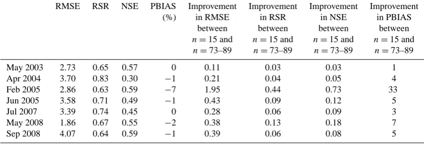
Table 3. The left-hand columns denote the RMSE, RSR, NSE and PBIAS for the model if the bootstrapping calculations of the end-member
concentrations were done using the whole data set (n=73–89). The improvement in the model performance when using the whole data set for calculating the end-member concentrations compared to n=15 is shown in the last four columns.
RMSE RSR NSE PBIAS Improvement Improvement Improvement Improvement (%) in RMSE in RSR in NSE in PBIAS
between between between between n=15 and n=15 and n=15 and n=15 and n=73–89 n=73–89 n=73–89 n=73–89
May 2003 2.73 0.65 0.57 0 0.11 0.03 0.03 1
Apr 2004 3.70 0.83 0.30 −1 0.21 0.04 0.05 4
Feb 2005 2.86 0.63 0.59 −7 1.95 0.44 0.73 33
Jun 2005 3.58 0.71 0.49 −1 0.43 0.09 0.12 5
Jul 2007 3.39 0.74 0.45 0 0.28 0.06 0.09 3
May 2008 1.86 0.67 0.55 −2 0.38 0.13 0.18 7
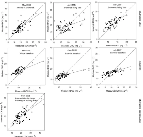
[image:6.595.87.507.558.701.2]Fig. 4. Modelled vs. measured DOC concentrations for the seven occasions. Catchments with peat coverage above 30 % are highlighted with
unfilled circles. The dashed line is the 1 : 1 line and the black line shows the regression line for all sites (black dots and unfilled circles).
projections to latent structures (PLS), to identify where and when the model failed to reproduce the measured data well. PLS is a method for relating two data matrices, X and Y, to each other by a linear multivariate model (Eriksson et al., 2006b). PLS is similar to principal component analysis (PCA), but instead of extracting the principal components so that they maximise the variance in the X matrix (as in PCA) the PLS method extracts the principal components so that they maximise the correlation between the X matrix and the Y matrix. The strength of the PLS method is the ability to analyse data with “many, noisy, collinear, and even incom-plete variables in both X and Y” (Eriksson et al., 2006b, a). The PLS analysis was conducted using the multivariate
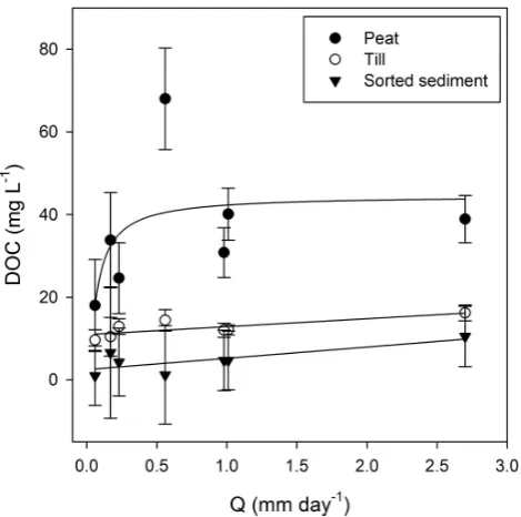
Fig. 5. End-member DOC concentrations as a function of
dis-charge. Error bars give the standard error for the bootstrapped end-member concentrations. Sorted sediment (R2=0.59, p=0.04) and till (R2=0.60,p=0.04) are described with linear relation-ships, and peat (R2=0.52,p=0.06) with an S-curve.
confidence interval) and the variable importance of the pro-jection (VIP) should be high (>1). In SIMCA-P+, for every model, the program also calculates the variable influence for each variable, called variable importance in the projection (VIP). VIP is the sum over all model dimensions. Variables with large VIP, larger than 1, are the most relevant for ex-plaining Y.
3 Results
The bootstrapping estimates of the end members show that peat has the highest DOC concentrations followed by till and lastly, fine sorted sediments (Table 1 and Fig. 5). Plot-ting the end-member concentration as a function of discharge for the sampling occasions revealed that the DOC concen-trations increased with discharge (Fig. 5). For silt and till this increase could be approximated by a linear relationship. For peat, the curve estimation procedure in PASW suggested a sigmoid curve (p <0.1). The standard error for the end-member concentration was low for till (on average 2 mg L−1)
but higher for peat and fine sorted sediments (on average 9 mg L−1), where sediment has the relatively highest stan-dard error (Fig. 5).
Figure 1 shows an example, from Sept 2008, of the mod-elled DOC concentrations using the landscape-mixing model combined with GIS and a high-resolution DEM. This shows the strength of this approach during a time when the model
performed well and could be used for prediction. With this approach, DOC concentrations can be modelled throughout an entire stream network based on a few headwater observa-tions. It is clear that many of the streams originate in peat-lands and have high concentrations initially. As the streams run into the area dominated by till and thin soils the concen-trations begin to decrease due to the intermediate concentra-tions from that composite landscape type. The streams drain-ing the sedimentary area in the valley have the lowest DOC concentrations and as these small streams mix into the larger main stream the concentrations continue to decrease towards the outlet.
The many measures used for evaluating model perfor-mance showed somewhat different results (Table 2). The root mean square error (RMSE) ranged from 2 to 5 mg L−1. Fol-lowing the guidelines from Moriasi et al. (2007) the RMSE-observation standard variation ratio (RSR) indicated that only two occasions are considered to be modelled satisfacto-rily (RSR<0.70). The mostly negative PBIAS values found (Table 2) indicate a general model overestimation bias. How-ever, using this measure all models performed reasonably well, except for the February 2005 data. The plotted mea-sured and modelled values (Fig. 4) and the slope indicate a systematic bias on all occasions, demonstrating that high DOC concentrations were underestimated and low concen-trations were overestimated in the model. The severity of this phenomenon varied and on three occasions the slope was judged to be good, while the other four occasions were judged to be unsatisfactory (baseflow and April 2004) (Ta-ble 2 and Fig. 4). According to the model evaluation guide-lines by Moriasi et al. (2007), based on the Nash–Sutcliffe ef-ficiency (NSE) measure only two models would be classified as satisfactory (NSE>0.5). To summarise, the many mea-sures of model efficiency gave different results and contained different information. The most suitable model fit measure depends on the question we are trying to answer. We believe that the RSR (standardised RMSE) and NSE (Nash–Sutcliffe efficiency) give the best overall description of the model per-formance. Taking into account all model performance mea-sures, the interpretation is that two models performed well (May 2003 and September 2008), one model performed un-satisfactorily (February 2005) and the rest performed satis-factorily.
3.1 Uncertainty
created fromn=15 sites. For most occasions, the model per-formance did not change substantially; including all sites to calculate the end-member concentrations only improved the model’s predictions by between 5 and 10 % (judged from im-provement in NSE) (Table 3). However, in the worst case (February 2005) the improvement was 73 %, indicating that the original construction data set sites were not representative for this occasion. This shows that there is room for model im-provement by increasing the number of observations used to calibrate the regression model. However, for this study we wanted to leave as many sites as possible for validation and analyses of the residuals.
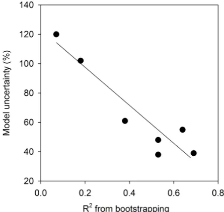
The second source of uncertainty was related to the un-certainty of the estimates of the end-member concentrations. Using the uncertainty from the bootstrapping estimates, a Monte Carlo analysis was performed to propagate the un-certainties into an overall uncertainty for the modelled val-ues. As expected, when there were difficulties in construct-ing a good bootstrappconstruct-ing model, indicated by lowR2for the model (Table 1, Fig. 6), the uncertainties of the modelled val-ues were high. The model uncertainty also affected its per-formance (tables 1 and 2 and Fig. 6). February 2005 had the highest uncertainty and had the worst model fit, while the models that performed best (May 2003 and September 2008) had a lower model uncertainty.
3.2 Residual analysis
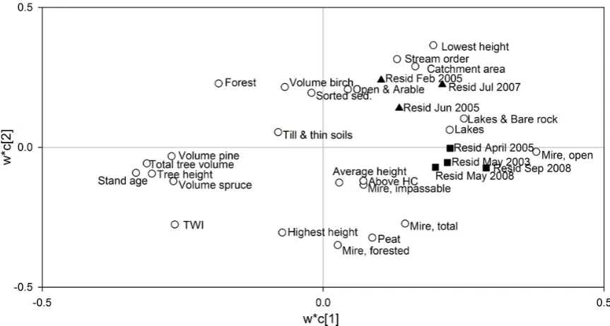
The first PLS model that gave an overview of the data had two significant components (R2Y = 0.35, R2X = 0.57, Q2 = 0.21) (Fig. 7). R2Y and R2X are goodness of fit mea-sures. That means that 57% of the variability inXwas used to explain 35 % of the variability in Y. Q2 is an estimate of the predictability of the model. It is calculated by cross-validation and resemblesR2in regression models where 0 is poor and 1 indicates optimal predictability. In a PLS load-ing plot, variables that lie close together co-vary, so the PLS analysis of the residuals (Fig. 7) showed that the residu-als clustered based on the discharge of the sampling oc-casion. The residuals from the high/intermediate flow sit-uations clustered along the first component (black squares in Fig. 7), while the residuals from baseflow measurements clustered higher along the second axis (black triangles in Fig. 7). In order to interpret which variables correlate with high residuals, two different models had to be constructed, one for high/intermediate flow, and one for baseflow condi-tions (Fig. 8).
[image:9.595.315.538.63.274.2]Both the model for the high/intermediate flow and the one for baseflow gave PLS models with one significant compo-nent. The models were refined to find the best predictor vari-ables, based on the conditions that the variable coefficient should be significant (95 % confidence interval, i.e. signifi-cance level of 0.05) and the variable importance of the pro-jection (VIP) should be high (>1). The models were then rerun on the selected variables to create two refined models
Fig. 6. The model uncertainty from the Monte Carlo analysis (%)
for the different occasions plotted against the coefficient of determi-nation (R2) for the bootstrapping models where the estimates were constructed.
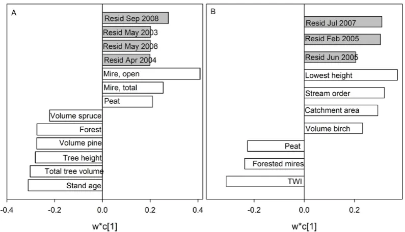
(Fig. 8a and b). The PLS analysis during high/intermediate discharge created a model with R2Y = 0.34, R2X = 0.66, and Q2 = 0.29 (Fig. 8a). That means that the variability in the 23 X variables could be reduced to one component, ex-plaining 34 % of the variability in Y. The nine significant X variables with a high weight explained 66 % of the vari-ability in the extracted component. The PLS loading plot shows the Y weights (c) and the X weights (w∗). The PLS easily handles many covariate variables (Fig. 8a); all X weights that correlate positively to Y weights are dif-ferent measures related to prevalence of peatlands, and all X weights that correlate negatively to Y weights are dif-ferent measures of the prevalence of forests. The interpreta-tion of Fig. 8a is that during high/intermediate discharge the landscape-mixing model overestimated the DOC concentra-tions from sub-catchments with a high coverage of peatlands, and underestimated DOC values in sub-catchments with a high proportion of forest. In contrast, the PLS loading plot for the residuals during baseflow (1 significant component, R2Y = 0.33, R2X = 0.50, Q2 = 0.26) (Fig. 8b) showed that the overestimated DOC concentrations were found in large low-elevation sub-catchments while the underestimated val-ues were those in sub-catchments dominated by peatlands.
4 Discussion
4.1 Selection of end members for the mixing model
Fig. 7. PLS loading plot for all stream DOC mixing-model residuals and associated catchment properties. Open circles denoteXvariables (catchment properties), black squares identify the residuals during high/intermediate discharge and black triangles indicate the residuals from baseflow occasions.
(Table 1, Fig. 5). Dissolved organic carbon in northern tem-perate and boreal streams is mostly of terrestrial origin, and peat-containing wetlands are often the major source of DOC (Creed et al., 2008; Dillon and Molot, 1997; Evans et al., 2007; Gergel et al., 1999; Walker et al., 2012). Streams draining the silty sediment area had the lowest concentra-tion, which can be explained by a combination of factors. In Krycklan, catchments underlain by silty sediments are lo-cated in the valley bottom of the lower-elevation larger catch-ments (Fig. 1). A combination of longer flow paths and a high subsurface water transit time can increase the decomposition of DOC (Wolock et al., 1997; Laudon et al., 2007). In addi-tion, a high specific surface area of the fine sorted sediments can lead to increased adsorption to mineral surfaces (Kalbitz et al., 2003).
As previously described, the mixing model is based on the assumption that the variability within a landscape type is smaller than between landscape types, and that different landscape elements generate different solute concentrations. This assumption was true during the high-flow situations, in-dicated by the separation of the error bars in Fig. 5, but during baseflow there was some overlap of the variability in the end members. Previous research has found that hydrology has a first-order control on the temporal variability of the DOC concentrations in streams (Hornberger et al., 1994; Seibert et al., 2009). Plotting the end-member concentrations as a function of discharge gave a slight positive relationship be-tween DOC and discharge for all landscape types (Fig. 5). We expected, but did not find, a negative relationship between DOC concentration and discharge in mire-dominated
catch-ments as suggested by other studies in the study area (Ågren et al., 2012) and in UK and Canada (Clark et al., 2007; Hin-ton et al., 1997). A likely reason for this is that the DOC dilution primarily occurs during the snowmelt period when large amounts of snowmelt water runoff as overland flow over frozen soil (Laudon et al., 2011). As we are including events driven by autumn rain and snowmelt, this seasonality difference will not be picked up by the model, but will in-stead provide a poorer model fit. It can be noted that we have not separated the signal from upland soils from the riparian soils in this study. The riparian zones are included in the sig-nal from both the forest on till soils and forest on sorted sedi-ment. However, till and sorted sediment soils have a different riparian DOC signal. Till soils usually have higher DOC con-centrations in the riparian soils (on humid and wet sites) than sediment soil. On humid and wet till soils we have a build-up of riparian peat; hence, water draining to a forest stream on till soils will pass through the riparian peat enriched in DOC and give a higher DOC signal to the forest stream than that of a dry till or a sorted sediment (Grabs et al., 2012).
Fig. 8. PLS loading plot showing the significant variables with high weight that explain the residuals in the stream DOC mixing model during (A) high–intermediate discharge and (B) baseflow. In each panel, positive values (bars to the right) indicate variables associated with sites
where DOC is overpredicted by the model, while negative values indicate variables associated with sites where DOC is underpredicted.
al. (2012) showed that the soil water concentrations from the fine sorted sediments riparian zones are low in Krycklan, averaging around 6 mg L−1. Furthermore, soil water DOC concentrations in dry till locations have also been found to be relatively low, on average 10 mg L−1, whereas they were 27 mg L−1 and 33 mg L−1 in humid and wet sites, respec-tively. By classifying the till-derived soils into three classes (dry, humid, wet) from the topographic wetness index we could potentially improve the predictability of the landscape-mixing model for DOC in the catchment. However, this mod-elling study did not aim to maximise the predictability of DOC in the landscape; instead, the residual analysis can be seen as a diagnostic tool to examine when and where simple land characteristics succeed in explaining the variability in DOC concentration on the landscape scale. Hence, this study should not be seen foremost as a predictive model but rather a learning framework for further development of our concep-tual understanding.
4.2 Landscape-mixing model performance
The landscape-mixing model (Cooper et al., 2004) combined with the high-resolution DEM offers a simple way of es-timating stream DOC concentrations throughout the stream network (Fig. 1) based on a few headwater observations. Whether the landscape-mixing model is good enough to be used for prediction depends on what the predictions are to be used for, and how much error is acceptable. However, our simple landscape-mixing model produces similar results to the more complicated process-based DOC-3 model (Jutras
4.3 Residual analysis
Using the landscape-mixing model as a baseline, the residual analysis can be used to identify other processes that regulate stream DOC. The residual analysis showed that the model failures were related to hydrological conditions (Fig. 7), indi-cating that different processes are important for stream DOC during low- vs. high-flow periods. During high/intermediate discharge the landscape-mixing model overestimated DOC in sub-catchments with a high peat coverage (Fig. 8a) while the model underestimated DOC in the same sub-catchments during baseflow (Fig. 8b). Higher concentrations from the wetland during baseflow and lower during high flow would have improved the model according to the residual analysis (Fig. 8a and b). A possible reason for the inability to predict the peatland–DOC relationship with high accuracy is that the model was constructed on a data set with peat coverage of 0–30 % while it was applied to sub-catchments in the valida-tion data set with a peat coverage of up to 55 % (highlighted as unfilled circles in Fig. 4). Another cause for the model underestimating high values and overestimating low values could be a dampening effect in the bootstrapping approach similar to other regression approaches (Gupta et al., 2009).
The PLS analysis of the residuals showed that during high/intermediate discharge (Fig. 8a) the model underesti-mates DOC in sub-catchments with much forest and overesti-mates DOC in sub-catchments with a high peat cover. Given that forests and peatlands are the most common landscape types in the study catchment this makes it difficult to interpret the results, because that means that forest and peatlands are highly correlated (Pearson correlation −0.94; p <0.001). This can create model artifacts as the overestimated DOC in forest-rich sub-catchments could be because of our inability to capture the true variability in peatland DOC, as discussed above. On the other hand, it could also be a causal relation-ship. Berggren et al. (2009) showed in a forest-mire gradient in the study area that mixed catchments change their dom-inant DOC source depending on discharge and that during high discharge the forests become more important as a DOC source.
It should be noted that the landscape-mixing model will only work, in the simple form applied here, if the concen-trations downstream are the result of simple mixing of up-stream water sources, i.e. if solute transport is conserva-tive. The residual analysis during low-flow situations shows that the mixing model overestimated the DOC concentra-tions in the lower lying large downstream catchments, with high stream order (Fig. 8b). This highlights the importance of including in-stream processes such as bacterial degrada-tion and/or photo-oxidadegrada-tion of DOC, as well as changing flow paths. These processes need to be included in the con-ceptual framework when modelling DOC during baseflow. Moody et al. (2013) recorded high photo-oxidation rates (ex-ceeding 10 mg C L−1day−1)during the first 1–2 days of ex-posure of fresh peat-derived DOC in UK headwater streams,
while Köhler et al. (2002) found photo-oxidation rates of the order of 2 mg L−1day−1 for water from a peat-dominated
headwater stream in the Krycklan catchment. In a companion study by Tiwari et al. (2014) we calculated the total photo-oxidation and bacterial degradation in the Krycklan stream channel network, from headwaters to the outlet, to be less than 1 mg L−1. Based on this analysis the bacterial degrada-tion and/or photo-oxidadegrada-tion of DOC could only partially ex-plain the overprediction of DOC at downstream sites during low flow.
During baseflow it was the large downstream catchments that had the highest overpredictions of DOC (Fig. 8b). The fact that this landscape type was significant only during base-flow indicates that the overprediction is related to chang-ing flow paths in large catchments durchang-ing baseflow. Lyon et al. (2012) have shown that there is considerable variability in specific discharge in the study catchment and that this af-fects the DOC exports to the different sites within the catch-ment. The water in the downstream main stem has a signal more similar to deep groundwater with low DOC concen-trations and high base cation concenconcen-trations (Klaminder et al., 2011). The overpredicted DOC concentration in the main stem of Krycklan could therefore be related to a large con-tribution of deeper low DOC groundwater at this scale, di-luting the DOC concentrations during baseflow situations. In a companion study by Tiwari et al. (2014) we quantified the amount of deeper groundwater input, using two separate techniques; a mass balance approach and a comparison of specific discharge between a headwater and the outlet. That study showed that at baseflow most of the water (80 %) at the outlet of Krycklan originated from deeper groundwater flow paths, so during low flow the DOC concentration was controlled by the groundwater concentrations and not from the water mixing down from the headwaters. The landscape-mixing model assumes that the water at the outlet is the sum of all contributing sources. To create a well-functioning model working during all flow situations one must therefore understand all contributing sources and how they vary dur-ing different hydrological situations. By includdur-ing the deep groundwater as a fourth end member (as a function of dis-charge) a landscape-mixing model could be constructed that predicts DOC concentrations throughout the stream network during all flow situations (R2=0.88, RMSE = 2.2 mg L−1) (Tiwari et al., 2014). This highlights the importance of under-standing changing flow paths and seasonal dynamics when modelling DOC in meso-scale catchments.
Acknowledgements. The study is a part of the Krycklan Catchment
Study (KCS) which is funded by The Swedish Research Council, Formas, ForWater, Future Forests, SKB, and the Kempe founda-tion, and involves many skilled, helpful scientists and students. Particular thanks go to the Krycklan crew for excellent field and lab support.
Edited by: B. A. Bergamaschi
References
Ågren, A., Buffam, I., Jansson, M., and Laudon, H.: Importance of seasonality and small streams for the landscape regulation of dissolved organic carbon export, J. Geophys. Res., 112, G03003, doi:10.1029/2006JG000381, 2007.
Ågren, A., Haei, M., Köhler, S. J., Bishop, K., and Laudon, H.: Regulation of stream water dissolved organic carbon (DOC) concentrations during snowmelt; the role of discharge, win-ter climate and memory effects, Biogeosciences, 7, 2901–2913, doi:10.5194/bg-7-2901-2010, 2010.
Ågren, A. M., Haei, M., Blomkvist, P., Nilsson, M. B., and Laudon, H.: Soil frost enhances stream dissolved organic carbon con-centrations during episodic spring snow melt from boreal mires, Glob. Change Biol., 18, 1895–1903, 2012.
Aitkenhead, J. A., Hope, D., and Billett, M. F.: The relationship between dissolved organic carbon in stream water and soil or-ganic carbon pools at different spatial scales, Hydrol. Process., 13, 1289–1302, 1999.
Berggren, M., Laudon, H., and Jansson, M.: Hydrological control of organic carbon support for bacterial growth in boreal headwater streams, Microb. Ecol., 57, 170–178, 2009.
Bishop, K., Buffam, I., Erlandsson, M., Fölster, J., Laudon, H., Seibert, J., and Temnerud, J.: Aqua Incognita: the unknown head-waters, Hydrol. Process., 22, 1239–1242, doi:10.1002/Hyp.7049, 2008.
Bloschl, G. and Sivapalan, M.: Scale Issues in Hydrologi-cal Modeling – a Review, Hydrol. Process., 9, 251–290, doi:10.1002/hyp.3360090305, 1995.
Buffam, I., Laudon, H., Seibert, J., Mörth, C. M., and Bishop, K.: Spatial heterogeneity of the spring flood acid pulse in a boreal stream network, Sci. Total Environ., 407, 708–722, doi:10.1016/j.scitotenv.2008.10.006, 2008.
Cey, E. E., Rudolph, D. L., Parkin, G. W., and Aravena, R.: Quanti-fying groundwater discharge to a small perennial stream in south-ern Ontario, Canada, J. Hydrol., 210, 21–37, doi:10.1016/S0022-1694(98)00172-3, 1998.
Clark, J. M., Lane, S. N., Chapman, P. J., and Adamson, J. K.: Ex-port of dissolved organic carbon from an upland peatland dur-ing storm events: Implications for flux estimates, J. Hydrol., 347, 438–447, 2007.
Cooper, D. M., Jenkins, A., Skeffington, R., and Gannon, B.: Catchment-scale simulation of stream water chemistry by spatial mixing: theory and application, J. Hydrol., 233, 121–137, 2000. Cooper, D. M., Helliwell, R. C., and Coull, M. C.: Predicting acid
neutralizing capacity from landscape classification: application to Galloway, south-west Scotland, Hydrol. Process., 18, 455– 471, doi:10.1002/Hyp.1320, 2004.
Creed, I. F. and Band, L. E.: Export of nitrogen from catchments within a temperate forest: Evidence for a unifying mechanism
regulated by variable source area dynamics, Water Resour. Res., 34, 3105–3120, 1998.
Creed, I. F., Sanford, S. E., Beall, F. D., Molot, L. A., and Dillon, P. J.: Cryptic wetlands: integrating hidden wetlands in regression models of the export of dissolved organic carbon from forested landscapes, Hydrol. Process., 17, 3629–3648, 2003.
Creed, I. F., Beall, F. D., Clair, T. A., Dillon, P. J., and Hesslein, R. H.: Predicting export of dissolved organic carbon from forested catchments in glaciated landscapes with shallow soils, Global Biogeochem. Cy., 22, Gb4024, doi:10.1029/2008gb003294, 2008.
D’Amore, D. V., Fellman, J. B., Edwards, R. T., and Hood, E.: Controls on dissolved organic matter concentrations in soils and streams from a forested wetland and sloping bog in southeast Alaska, Ecohydrology, 3, 249–261, 2010.
Dawson, J. J. C., Tetzlaff, D., Speed, M., Hrachowitz, M., and Soulsby, C.: Seasonal controls on DOC dynamics in nested up-land catchments in NE Scotup-land, Hydrol. Process., 25, 1647– 1658, 2011.
Dillon, P. J. and Molot, L. A.: Effect of landscape form on export of dissolved organic carbon, iron, and phosphorus from forested stream catchments, Water Resour. Res., 33, 2591–2600, 1997. Eriksson, L., Johansson, E., Kettaneh-Wold, N., Trygg, J.,
Wik-ström, C., and Wold, S.: Multi- and Megavariate Data Analysis, Part II Advanced Applications and Method Extentions, Umetrics, Umeå, Sweden., 307 pp., 2006a.
Eriksson, L., Johansson, E., Kettaneh-Wold, N., Trygg, J., Wik-ström, C., and Wold, S.: Multi- and Megavariate Data Analysis, Part I Bacis Principles and Applications, Umetrics, Umeå, Swe-den, 425 pp., 2006b.
Evans, C. D., Cooper, D. M., and Gannon, B.: A Novel Method for Mapping Critical Loads Across a River Network: Application to the River Dart, Southwest England, Water, Air Soil Poll., 1, 437– 453, doi:10.1023/a:1011546930939, 2001.
Evans, C. D., Freeman, C., Cork, L. G., Thomas, D. N., Reynolds, B., Billett, M. F., Garnett, M. H., and Norris, D.: Evidence against recent climate-induced destabilisation of soil carbon from C-14 analysis of riverine dissolved organic matter, Geo-phys. Res. Lett., 34, L07407, doi:10.1023/a:1011546930939, 2007.
Forsum, A., Laudon, H., and Nordin, A.: Nitrogen uptake by Hy-locomium splendens during snowmelt in a boreal forest, Eco-science, 15, 315–319, 2008.
Gergel, S. E., Turner, M. G., and Kratz, T. K.: Dissolved organic car-bon as an indicator of the scale of watershed influence on lakes and rivers, Ecol. Appl., 9, 1377–1390, 1999.
Grabs, T., Seibert, J., Bishop, K., and Laudon, H.: Modeling spa-tial patterns of saturated areas: A comparison of the topographic wetness index and a dynamic distributed model, J. Hydrol., 373, 15–23, 2009.
Grabs, T., Bishop, K., Laudon, H., Lyon, S. W., and Seibert, J.: Riparian zone hydrology and soil water total organic car-bon (TOC): implications for spatial variability and upscaling of lateral riparian TOC exports, Biogeosciences, 9, 3901–3916, doi:10.5194/bg-9-3901-2012, 2012.
Haei, M., Öquist, M. G., Buffam, I., Ågren, A., Blomkvist, P., Bishop, K., Löfvenius, M. O., and Laudon, H.: Cold winter soils enhance dissolved organic carbon concentrations in soil and stream water, Geophys. Res. Lett., 37, L08501, doi:10.1029/2010gl042821, 2010.
Hinton, M. J., Schiff, S. L., and English, M. C.: The significance of storms for the concentration and export of dissolved organic car-bon from two Precambrian Shield catchments, Biogeochemistry, 36, 67–88, 1997.
Hornberger, G. M., Bencala, K. E., and Mcknight, D. M.: Hydrolog-ical Controls on Dissolved Organic-Carbon During Snowmelt in the Snake River near Montezuma, Colorado, Biogeochemistry, 25, 147–165, 1994.
Inamdar, S. P., Christopher, S. F., and Mitchell, M. J.: Export mech-anisms for dissolved organic carbon and nitrate during summer storm events in a glaciated forested catchment in New York, USA, Hydrol. Process., 18, 2651–2661, 2004.
Jutras, M. F., Nasr, M., Castonguay, M., Pit, C., Pomeroy, J. H., Smith, T. P., Zhang, C. F., Ritchie, C. D., Meng, F. R., Clair, T. A., and Arp, P. A.: Dissolved organic carbon concentrations and fluxes in forest catchments and streams: DOC-3 model, Ecol. Model., 222, 2291–2313, doi:10.1016/j.ecolmodel.2011.03.035, 2011.
Kalbitz, K., Schmerwitz, J., Schwesig, D., and Matzner, E.: Biodegradation of soil-derived dissolved organic matter as re-lated to its properties, Geoderma, 113, 273–291, 2003.
Klaminder, J., Grip, H., Mörth, C. M., and Laudon, H.: Carbon min-eralization and pyrite oxidation in groundwater: Importance for silicate weathering in boreal forest soils and stream base-flow chemistry, Appl. Geochem., 26, 319–324, 2011.
Knorr, K.-H.: DOC-dynamics in a small headwater catchment as driven by redox fluctuations and hydrological flow paths – are DOC exports mediated by iron reduction/oxidation cycles?, Bio-geosciences, 10, 891–904, doi:10.5194/bg-10-891-2013, 2013. Köhler, S., Buffam, I., Jonsson, A., and Bishop, K.: Photochemical
and microbial processing of stream and soilwater dissolved or-ganic matter in a boreal forested catchment in northern Sweden, Aquat. Sci., 64, 269–281, 2002.
Köhler, S. J., Buffam, I., Laudon, H., and Bishop, K. H.: Cli-mate’s control of intra-annual and interannual variability of to-tal organic carbon concentration and flux in two contrasting bo-real landscape elements, J. Geophys. Res.-Biogeo., 113, 03012, doi:10.1029/2007JG000629, 2008.
Laudon, H., Sjöblom, V., Buffam, I., Seibert, J., and Mörth, M.: The role of catchment scale and landscape characteristics for runoff generation of boreal streams, J. Hydrol., 344, 198–209, 2007. Laudon, H., Berggren, M., Ågren, A., Buffam, I., Bishop, K., Grabs,
T., Jansson, M., and Köhler, S.: Patterns and Dynamics of Dis-solved Organic Carbon (DOC) in Boreal Streams: The Role of Processes, Connectivity, and Scaling, Ecosystems, 14, 880–893, doi:10.1007/s10021-011-9452-8, 2011.
Laudon, H., Buttle, J., Carey, S. K., McDonnell, J., McGuire, K., Seibert, J., Shanley, J., Soulsby, C., and Tetzlaff, D.: Cross-regional prediction of long-term trajectory of stream water DOC response to climate change, Geophys. Res. Lett., 39, L18404, doi:10.1029/2012gl053033, 2012.
Laudon, H., Taberman, I., Ågren, A., Futter, M., Ottosson-Löfvenius, M., and Bishop, K.: The Krycklan Catchment Study—A flagship infrastructure for hydrology,
biogeochem-istry, and climate research in the boreal landscape, Water Resour. Res., 49, 7154–7158, doi:10.1002/wrcr.20520, 2013.
Lyon, S. W., Nathanson, M., Spans, A., Grabs, T., Laudon, H., Tem-nerud, J., Bishop, K. H., and Seibert, J.: Specific discharge vari-ability in a boreal landscape, Water Resour. Res., 48, W08506, doi:10.1029/2011WR011073, 2012.
Mattsson, T., Kortelainen, P., Laubel, A., Evans, D., Pujo-Pay, M., Raike, A., and Conan, P.: Export of dissolved organic matter in relation to land use along a European climatic gradient, Sci. Total Environ., 407, 1967–1976, 2009.
Moody, C. S., Worrall, F., Evans, C. D., and Jones, T.: The rate of loss of dissolved organic carbon (DOC) through a catchment, J. Hydrol., 492, 139–150, 2013.
Moriasi, D. N., Arnold, J. G., Van Liew, M. W., Bingner, R. L., Harmel, R. D., and Veith, T. L.: Model evaluation guidelines for systematic quantification of accuracy in watershed simulations, T. ASABE, 50, 885–900, 2007.
Mulholland, P.: Large-scale patterns in dissolved organic carbon concentration, flux, and sources, in: Aquatic Ecosystems: Inter-activity of Dissolved Organic Matter, edited by: Findlay, S. E. G. and Sinsabaugh, R. L., Academic Press, New York, 139–159, 2003.
Oni, S. K., Futter, M. N., Bishop, K., Köhler, S. J., Ottosson-Löfvenius, M., and Laudon, H.: Long-term patterns in dis-solved organic carbon, major elements and trace metals in boreal headwater catchments: trends, mechanisms and heterogeneity, Biogeosciences, 10, 2315–2330, doi:10.5194/bg-10-2315-2013, 2013.
Pacific, V. J., Jencso, K. G., and McGlynn, B. L.: Variable flushing mechanisms and landscape structure control stream DOC export during snowmelt in a set of nested catchments, Biogeochemistry, 99, 193–211, doi:10.1007/s10533-009-9401-1, 2010.
Rantakari, M., Mattsson, T., Kortelainen, P., Piirainen, S., Finer, L., and Ahtiainen, M.: Organic and inorganic carbon concentra-tions and fluxes from managed and unmanaged boreal first-order catchments, Sci. Total Environ., 408, 1649–1658, 2010. Raymond, P. A. and Saiers, J. E.: Event controlled DOC export from
forested watersheds, Biogeochemistry, 100, 197–209, 2010. Seibert, J., Grabs, T., Köhler, S., Laudon, H., Winterdahl, M.,
and Bishop, K.: Linking soil- and stream-water chemistry based on a Riparian Flow-Concentration Integration Model, Hydrol. Earth Syst. Sci., 13, 2287–2297, doi:10.5194/hess-13-2287-2009, 2009.
Tank, S. E., Frey, K. E., Striegl, R. G., Raymond, P. A., Holmes, R. M., McClelland, J. W., and Peterson, B. J.: Landscape-level controls on dissolved carbon flux from diverse catchments of the circumboreal, Global Biogeochem. Cy., 26, GB0E02, doi:10.1029/2012GB004299, 2012.
Temnerud, J. and Bishop, K.: Spatial variation of streamwater chemistry in two Swedish boreal catchments: Implications for environmental assessment, Environ. Sci. Technol., 39, 1463– 1469, 2005.
Temnerud, J., Seibert, J., Jansson, M., and Bishop, K.: Spatial varia-tion in discharge and concentravaria-tions of organic carbon in a catch-ment network of boreal streams in northern Sweden, J. Hydrol., 342, 72–87, 2007.
of model uncertainties, Water Resour. Res., 50, 514–525, doi:10.1002/2013wr014275, 2014.
Walker, C. M., King, R. S., Whigham, D. F., and Baird, S. J.: Land-scape and Wetland Influences on Headwater Stream Chemistry in the Kenai Lowlands, Alaska, Wetlands, 32, 301–310, 2012. Wolock, D. M., Fan, J., and Lawrence, G. B.: Effects of basin size
on low-flow stream chemistry and subsurface contact time in the Neversink River Watershed, New York, Hydrol. Process., 11, 1273–1286, 1997.