A quantitative study of magnetospheric magnetic field line deformation by a two-loop substorm current wedge

www.ann-geophys.net/33/505/2015/ doi:10.5194/angeo-33-505-2015

© Author(s) 2015. CC Attribution 3.0 License.

A quantitative study of magnetospheric magnetic field line

deformation by a two-loop substorm current wedge

A. V. Nikolaev1, V. A. Sergeev1, N. A. Tsyganenko1, M. V. Kubyshkina1, H. Opgenoorth2, H. Singer3, and V. Angelopoulos4

1_{Department of Earth Physics, Saint Petersburg State University, Petrodvoretz, Russia} 2_{Uppsala Division, Swedish Institute of Space Physics, Uppsala, Sweden}

3_{Space Weather Prediction Center, NOAA, Boulder, Colorado, USA}

4_{Department of Earth, Planetary, and Space Sciences and Institute of Geophysics and Space Physics,} University of California, Los Angeles, California, USA

Correspondence to: A. V. Nikolaev ([email protected])

Received: 24 September 2014 – Revised: 8 March 2015 – Accepted: 2 April 2015 – Published: 29 April 2015

Abstract. Substorm current wedge (SCW) formation is as-sociated with global magnetic field reconfiguration during substorm expansion. We combine a two-loop model SCW (SCW2L) with a background magnetic field model to in-vestigate distortion of the ionospheric footpoint pattern in response to changes of different SCW2L parameters. The SCW-related plasma sheet footprint shift results in forma-tion of a pattern resembling an auroral bulge, the pole-ward expansion of which is controlled primarily by the to-tal current in the region 1 sense current loop (I1). The mag-nitude of the footprint latitudinal shift may reach ∼10◦ corrected geomagnetic latitude (CGLat) during strong sub-storms (I1=2 MA). A strong helical magnetic field around the field-aligned current generates a surge-like region with embedded spiral structures, associated with a westward trav-eling surge (WTS) at the western end of the SCW. The helical field may also contribute to rotation of the ionospheric pro-jection of narrow plasma streams (auroral streamers). Other parameters, including the total current in the second (region 2 sense) loop, were found to be of secondary importance. Ana-lyzing two consecutive dipolarizations on 17 March 2010, we used magnetic variation data obtained from a dense midlati-tude ground network and several magnetospheric spacecraft, as well as the adaptive AM03 model, to specify SCW2L pa-rameters, which allowed us to predict the magnitude of pole-ward auroral expansion. Auroral observations made during the two substorm activations demonstrate that the SCW2L combined with the AM03 model nicely describes the az-imuthal progression and the observed magnitude of the

au-roral expansion. This finding indicates that the SCW-related distortions are responsible for much of the observed global development of bright auroras.

Keywords. Magnetospheric physics (auroral phenomena; current systems; storms and substorms)

1 Introduction

There-closer to Earth. The single-wedge model thus becomes a two-loop (quadrupolar FAC) SCW model (SCW2L) (Sergeev et al., 2014a). Magnetohydrodynamic simulations of magneto-tail reconnection (Birn and Hesse, 1999; Birn and Hesse, 2014), the recent equilibrium Rice Convection Model (RCM-E), and flow burst simulations (Yang et al., 2012) consistently show that a plasma pressure increase in front of the earth-ward flow channel is responsible for generation of this addi-tional R2 loop. From observations, Liu et al. (2013) inferred quadrupolar FACs by analyzing individual propagating flow bursts, while Sergeev et al. (2011) and Sergeev et al. (2014a) showed them to be consistent with SCW-related magnetic perturbations by comparing multipoint observations in the near magnetosphere and at ground midlatitudes during sub-storms.

During strong substorms, the total SCW current may ex-ceed 1 MA and thus may significantly change magneto-spheric configuration and ionomagneto-spheric mapping in the near-Earth region. At the same time, intense FAC sheets (es-pecially upward FACs) accelerate precipitating electrons that cause bright auroras (Waters et al., 2001). Therefore, substorm-related magnetic reconfiguration and associated changes in field-line mapping from the magnetosphere to the ionosphere should be reflected in an auroral pattern redistri-bution, which, in turn, can provide information about these changes. An example is poleward auroral expansion accom-panied by formation of a bulge of bright auroras. This basic signature of the substorm expansion phase has been tradi-tionally related to electric current disruption and magnetic reconnection in the magnetotail (e.g., Roux et al., 1991; Yah-nin et al., 2006; Kubyshkina et al. 2011). The relationship is based on rather limited evidence however (see, e.g., summary by Keiling et al., 2012). The quantitative evaluation of the role of FACs in variable patterns of field-line mapping during substorm-related dipolarization and auroral expansion, an in-teresting exercise, has been addressed in a few previous pa-pers. Those studies, however, utilized highly idealized SCW models with infinitely thin line currents flowing along either dipolar or early empirical model field lines (Vasilyev et al., 1986; Kaufmann and Larson, 1989; Tsyganenko, 1997), or used dipolarization effects to represent a global tail recon-figuration (Kubyshkina et al., 2011). Because SCW effects on the magnetotail configuration and mapping by applying

cellent spacecraft coverage in the magnetosphere.

2 Modeling of the ionospheric footprint displacement produced by the substorm current wedge

2.1 Brief description of the SCW2L model

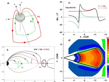
Here we use the SCW2L model, which was presented, tested, and extensively discussed by Sergeev et al. (2014a) (here-after referred to as Paper 1). It includes two pairs of field-aligned currents: the high-latitude R1 loop and the more earthward/equatorward R2 loop (see Fig. 1a). When com-bined, these loops form a quadrupolar FAC source near the ionosphere. The model was developed for substorm case studies to quantitatively evaluate the intensities of both R1 (I1)and R2 (I2) currents, based on observations. Its input includes the dipolarization amplitude (1BZ) in the

magne-tosphere, measured by a few spacecraft, and the amplitudes of1Xand1Y components of bay-like variations, measured at several ground midlatitude observatories. As discussed in Paper 1 and illustrated in Fig. 1c, the magnitude1BZin the

magnetosphere is rather uniform over most of the dipolar-ized region, that is, in the area between the R1 and R2 loops (red hatching in Fig. 1d). Here1BZ is mostly sensitive to

the magnitude of R1 current (I1)and allows one to evalu-ate its magnitude, whereas the midlatitude ground variations respond to the net current (I1+I2), so the combination of two (magnetospheric and ground-based) inputs is necessary to evaluate bothI1andI2parameters.

Because of the scarcity of magnetospheric spacecraft ob-servations, the model should be as simple as possible. In particular, both R1 and R2 loops are assumed to occupy the same azimuthal sector, which is roughly consistent with simulation results presented by Yang et al. (2012) and Birn and Hesse (2013). In our case, we use the filamentary cur-rent model with the curcur-rent transverse spread specified as

Figure 1. (a) Illustration of the two-loop SCW model (SCW2L); (b) magnetic field-line topology when the background (T89+IGRF) magnetic field (shown by current-carrying red/green lines) is compared to field lines (black lines) after the addition of SCW2L; (c) partial contribution to1BZ perturbations of R1 (red) and R2 (green) SCW components and their sum (black line); (d)1BZ distribution in the

equatorial plane in the SCW2L model (adapted from Sergeev et al., 2014a). All illustrations are done for a 60◦wide wedge withI1=1 MA andI2=0.5 MA.

With RCF=0, an equatorial point at XGSM= −15 RE, YGSM=0 in the neutral sheet maps to geomagnetic lati-tude of∼70◦GLat in the ionosphere, while setting RCF=6 moves the footprint down to ∼63◦GLat (see also Sergeev et al. (2011) for the detailed description of RCF parame-ter). Using the filamentary model rather than the azimuthally distributed field-aligned currents does not significantly af-fect1BZin the dipolarized region, except in the immediate

vicinity of the FAC filament (see Fig. 3 and supplementary plots S1–S3 in Sergeev et al., 2014a). Also, in our analy-ses below we set the distance to the equatorial current of the R1 loop to RT1=15 Re (see also parameter descriptions in Fig. S1 in the Supplement).

Figure 1b illustrates the applicability domain of the SCW2L model, limited primarily to the inner magneto-sphere, where the model is intended to faithfully describe the dipolarization effects. Close to the filamentary equatorial R1 current and beyond it, the model cannot provide a realistic description of electric currents flowing in the reconnecting plasma sheet. Nevertheless, as shown in Paper 1, the ampli-tude and distribution of the dipolarization ampliampli-tude1BZin

the inner region (earthward of 12 Re) depends only slightly on the exact location and radial distribution of the equatorial R1 current. If the peak perturbation from the equatorial fila-ment exceeds the background BZ value, a closed field line

loop is formed around the filament (Fig. 1b). In addition, a region with southward total BZ that is topologically

dis-connected from the ionosphere is formed tailward of the R1 filament. These two model artifacts should be kept in mind when analyzing SCW2L-related deformation and magnetic field-lines mapping.

2.2 SCW2L-related deformations

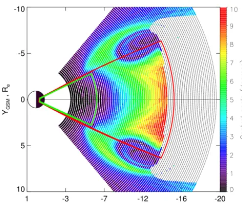
Figure 2. Magnetospheric pattern of neutral sheet footprint

geo-centric angular displacement (color coded) caused by addition of the SCW2L model to the T89+IGRF models. The SCW2L model parameters were set as follows: I1=1 MA, I2=0.5 MA, RT1=15 Re, RT2=6 Re, RCF=6, and the wedge azimuthal width 50◦.

contribution added. The azimuthal and longitudinal shift be-tween the footpoints

α=cos−1 _x

1x2+y1y2+z1z2 R2

, (1)

serves as a quantitative measure of the SCW mapping effect. HereR=1.02 Re, and [x1,y1,z1] and [x2,y2,z2] are foot-print Cartesian coordinates, obtained from the two tracings. An example of the footprint shift distribution in the equato-rial plane is shown in Fig. 2; each point on the arc is colored according to itsαvalue. As mentioned above, the valid area in our analysis is the region earthward of the R1 equatorial current between the upward and downward FACs and col-ored in green and red lines. No ionospheric footpoints exist tailward of that area (grey color) because the corresponding field lines either belong to the magnetic “island” inside the loop or map tailward.

The equatorial diagram of the footpoint shifts should be viewed with the ionospheric mapping pattern shown in Fig. 3 aimed to characterize its geometry. At the ionospheric level, we show two families of reference equatorial equidistant arcs mapped to the ionosphere using only the background model field (red contours) as well as the background and the SCW2L field (green curves). Such a representation, which helps to show different types of magnetic field deformation; it is especially useful when discussing possible auroral im-plications.

Comparing Figs. 2 and 3 reveals three specific regions of footprint deformation. The first, the most important region inside the dipolarized region, lies between the equatorial R1

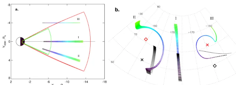
Figure 3. Ionospheric mapping of equatorial geocentric circle

arcs (equatorial distance is labeled for selected circles). The red lines show neutral sheet mapping using the T89+IGRF model; the green lines show mapping of the same points using the SCW2L+T89+IGRF model. Ionospheric locations of upward (downward) FACs are indicated by diamond (cross) symbols. The SCW2L model is the same as in Fig. 2.

and R2 currents. Here the SCW2L-related 1BZ

perturba-tions are significantly larger than the backgroundBZ

com-ponent (BZ0): the traced field lines pass at larger distances from the neutral sheet plane (see Fig. 1b) and hence land at higher latitudes. At the ionospheric level, the dipolarization region corresponds to the area of significant poleward shift of the footpoints. In the example illustrated in Figs. 2 and 3, this shift can reach up to 8◦corrected geomagnetic latitude (CGLat) at the center of the SCW. Because of an increase in the1BZ/ BZ0ratio, the magnitude of the poleward ex-pansion increases as the equatorial point approaches the R1 filament.

The second region corresponds to the field-line twisting area around the intense R1 field-aligned current filament, which is well represented by the spiral-like shapes in Fig. 3. Initially located within the wedge close to the filament axis, the points are significantly twisted, but their resulting foot-point displacements appear to be small, forming the blue ar-eas near the FACs (between 8 and 14 Re along thex axis) in Fig. 2. Contradictions between the amount of footprint movement and smallαvalues appear in the cases when foot-points rotate around FACs and return close to the original location. The combination of type 1 and type 2 deformations produces a large-scale poleward bulge-like structure in the ionospheric projection of the magnetospheric dipolarization region, which may be associated with the auroral bulge.

mag-netosphere, where the R2 loop is formed and (2) an R2 cur-rent that is smaller than the R1 curcur-rent.

For auroral research, it is also instructive to map an-other type of neutral sheet contour. Rather than arc-like seg-ments, one may consider rectilinear strips oriented along the

x axis plasma flow geometry (Fig. 4a) and created as az-imuthally localized partitions of the neutral sheet described in Sect. 2.2. The distorted ionospheric projections of these strips can be likened to elementary structures associated with auroral arcs or other features observed at low altitudes. One such structure can be an ionospheric projection of nar-row (2–3 Re wide across the tail), fast plasma streams, also known as “bursty bulk flows” (BBFs) (Baumjohann et al., 1990; Angelopoulos et al., 1992), which are associated with a family of approximately north–south aligned auroral arcs (or auroral streamers, or poleward boundary intensifications, PBIs) (e.g., Elphinstone et al., 1996; Henderson et al., 1998; Lyons et al., 1999; Nakamura et al., 2001; Henderson, 2012, and references therein). Figure 4a shows an equatorial view of three line segments (I and II contours) in the dipolar-ized region, which simulate three hypothetical fast earthward plasma streams. Although their mapped images look simi-lar, if mapped along the background magnetic field (Fig. 4b, black contours), adding the SCW2L contribution causes a significant deformation of the image. Although it is shifted poleward and somewhat elongated, the shape of the stream located at the central wedge meridian (Y =0, contour I) does not change much. The shape of the off-center contours (II), however, changes considerably, including a significant rota-tion of the mapped structure. Although the general features of the deformation are recognizable with the help of Fig. 3, the amount of rotation and the scale of the crescent-like structure depend on many details of structure location relative to the wedge field-aligned currents. In particular, the footpoints of the dawnside stream that crosses the equatorial projection of the wedge (but does not intersect the FAC flux tube) are sub-ject to stronger rotation than those of a non-crossing duskside stream. In addition, the latitude of the stream endpoint (the most earthward) is roughly 4◦CGLat southward of the non-crossing stream’s endpoint. Investigation of corresponding auroral patterns may have interesting implications for stud-ies of the FAC strength and distribution.

2.3 Poleward footpoint expansion as a function of SCW parameters

In this section, we investigate poleward shifts of ionospheric footpoints traced from the neutral sheet at the central wedge meridian (hereY =0,Z=0) using different SCW2L param-eter values. Values of the SCW2L spatial paramparam-eters, such as

PW,PE, RT1, and RT2, are similar to those used in the pre-vious section. Characterizing the event strength by a com-bination of R1 current intensity (I1)and field-line stretch-ing amplitude (RCF), we select combinations correspond-ing to different magnetic disturbance levels as follows: weak

substormsI1=0.5 MA, RCF=3 (Fig. 5c); moderate sub-stormsI1=1 MA, RCF=6 (Fig. 5d); and strong substorms I1=2 MA, RCF=8 (Fig. 5e). To set the RCF dependence onI1, we relied on Fig. 10 in Sergeev et al. (2014a), which demonstrated a statistical relationship between dipolarization amplitudes andBZ0at geosynchronous distance prior to the dipolarization onset and suggestedI2/ I1=0.5.

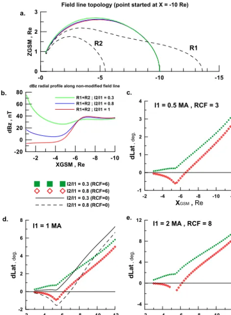
As seen from Fig. 5c, d, and e, the parameter that effec-tively controls magnitude of poleward expansion is the in-tensity of the R1 current. The computed maximal poleward shift of ionospheric footpoints at the wedge central merid-ian is rather small in the case of weak substorm (1Lat∼2– 3◦CGLat). It increases under moderate substorm conditions (1Lat∼5–6◦CGLat) and can reach1Lat∼10◦CGLat dur-ing highly disturbed events. Such values look quite realistic when compared to the known magnitudes of the auroral pole-ward expansion during substorms (Akasofu, 1976).

Surprisingly, the growth of the R2 current (increase in the

I2/ I1ratio under a fixed value ofI1), which enhances the dipolarization in the equatorial plane (see Fig. 1c, d, and e), actually decreases footprint shifts, resulting in a∼20 % smaller latitudinal expansion. This is explained by Fig. 5b, which shows the wedge-related1BZ at locations along the

magnetic field line, corresponding to the T89+IGRF model and starting in the middle of the wedge fromX= −10 Re,

Z=0. Figure 5b shows that the increase inI2actually sup-presses 1BZ in the high-latitude part of the field line (at

small radial distances, R< 6 Re), without a substantial in-crease in1BZat its near-equatorial (R> 6 Re) part. The

con-figuration of such a distorted field line is illustrated in Fig. 5a. According to Fig. 5c, d, and e, the equatorial bulge caused by the R2 current is virtually absent whenI2/ I1 is small (=0.3) and has a relatively small magnitude (<∼1◦_1Lat)

whenI2/ I1=0.8.

As shown in Fig. 5d, the role of background field line stretching is also very modest. The stretch increase from RCF=3 to 6 reduces the ionospheric shift in the region of strong magnetic gradients (near the R1 and R2 type currents) by1Lat∼1–2◦CGLat. This can be partly due to changing magnitudes of the backgroundBZ0at different RCF, which resulted in an equatorward shift of the field-line footpoints. 3 SCW and poleward auroral expansion during the 17

March 2010 substorm

Figure 4. (a) Equatorial locations of three hypothetical narrow plasma streams; (b) their ionospheric footprints. The black strips indicate

stream mapping using the background IGRF+T89 model; the colored strips represent stream mapping in the IGRF+T89+SCW2L model (I1=1 MA,I2=0.5 MA, R1=15 Re, RT2=6 Re and RCF=6). Color coding indicates the streamers, spatial orientation or movement direction.

and its spacecraft-based modeling (including SCW2L runs) are described in detail in a companion paper by Sergeev et al. (2014b). Here we briefly restate some of their results and concentrate on the mapping issues.

The inversion modeling was performed in two stages. In the first, we used the well-known magnetogram inversion al-gorithm (Sergeev et al., 1996) with a simple (based on dipo-lar field lines) SCW model and with input from 20 mid-latitude magnetic observations, to infer the parameters of the SCW, symmetric (DR), and partial (DRP) ring current systems (the latter two systems changed little during that event, and their effect is not discussed here). In the sec-ond, we used values of westward (PW) and eastward (PE) SCW longitudes, obtained in the previous step, and ran the inversion procedure based on a combination of midlat-itude ground-based data, spacecraft observations, and the ad-vanced SCW2L model (see also Fig. S1 in the Supplement). The inversion algorithm usually searched for and found a global minimum of a fit functionσ:

σ =KST

X 1XOBS

KIND

−1XMOD

2

+

_1Y OBS

KIND

−1YMOD

2!

(2)

+KSC

X

(1BZobs−1BZmod)2,

where the indices “obs” and “mod” stand for the ob-served and modeled fields, respectively, and KIND=1.5 is the induction correction coefficient. The summation is car-ried out over the NST stations and NSC spacecraft, and KST and KSC are the weight coefficients needed to bal-ance the contributions to the minimized target function (i.e.,

KST×NST=KSC×NSC)from a large number of stations (NST=19) and a small number of spacecraft located in-side the dipolarized region (NSC=1 or 2). Throughout that run, we kept some parameters fixed, including RT1=15 Re,

RTDRP=13 Re, and RDR=4 Re. We made equatorial dis-tance to R2 current free and varied RT2parameter between 5.5 and 6 Re.

As a result, we evaluated theI1,I2, and I3 (DRP) cur-rents for two consecutive dipolarizations with the activity starting at T =04:56 UT (reference level, start time of ac-tivation no. 1) and T =05:36 UT (start time of activation no. 2). The reference level for both activations was chosen at T0=04:56 UT because the second activation started dur-ing the recovery from the first activation. The observed and modeled field perturbations during the peaks of two activa-tions are compared in Fig. 6. This figure demonstrates good agreement between the observed and predicted dipolariza-tion magnitudes, namely 1BZ in the bottom right panels

for spacecraft dipolarization and1X and1Y components in the left panels for ground stations. We also ran the adap-tive model AM03 (see also Sergeev et al. (2014b) for more details), which uses the T96 model equations but adjusts their parameters to provide a best fit to the magnetic field observed during the event of interest.

Using the inversion results, we can now predict the map-ping using realistic parameters of the SCW2L model cur-rent system as we did in Sect. 2.2 (Figs. 7 and 8). The AM03+IGRF model at 04:56 UT is used here as the back-ground field model. Colored patterns in Fig. 7 illustrate the degree of footprint distortion (similarly to Fig. 2) for two dipolarization maxima epochs at 05:13 UT (left panel, event no. 1) and 05:50 UT (right panel, event no. 2).

-2 -4 -6 -8 -10 -12 XGSM , Re

-1 0 1 2 3 4 d L at , de g.

-2 -4 -6 -8 -10 -12 XGSM , Re

-2 0 2 4 6 8 d L at , de g.

I2/I1 = 0.3 (RCF=6) I2/I1 = 0.8 (RCF=6) I2/I1 = 0.3 (RCF=0) I2/I1 = 0.8 (RCF=0)

-2 -4 -6 -8 -10 -12 XGSM , Re

-4 0 4 8 12 d L at , de g.

I1 = 2 MA , RCF = 8 I1 = 0.5 MA , RCF = 3

-2 -4 -6 -8 -10

XGSM , Re -20 0 20 40 60 80 d B z , n T

R1+R2 ; I2/I1 = 0.3 R1+R2 ; I2/I1 = 0.8 R1+R2 ; I2/I1 = 1 dBz radial profile along non-modified field line

-0 -5 -10 -15

0 1 2 3 Z G S M , R e

Field line topology (point started at X = -10 Re)

R2

R1

I1 = 1 MA a.

b. c.

d. e.

Figure 5. Parameter dependence of footprint displacement. (a) The

X0Z plane projection of SCW2L FACs (dashed lines) and mag-netic field line traced from X= −10 Re; (b) 1BZ generated by

SCW2L (I₁=1 MA) along the T89 magnetic field line start-ing at X= −10 Re; (c) latitudinal shifts for weak substorms (I1=0.5 MA, RCF=3); (d) same panel for strong events with two different magnetotail stretches (I1=1 MA, RCF=0 and 6);

(e) same as (c) and (d) but calculated for extremely strong

sub-storms (I1=2 MA, RCF=8). Different colors in panels (c–e) cor-respond to the same I1but with two values of theI2/ I1current ratio, shown in green forI2/ I1=0.3 and in red forI2/ I1=0.8. All calculations are done for the fixed RT1=15 Re, RT2=6 Re, wedge azimuthal width of 50◦.

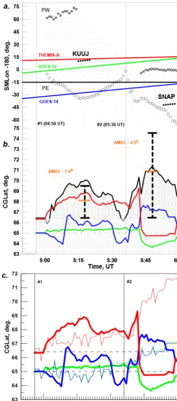
atX= −11 Re ,Y =3 Re, andZ= −1.56 Re through both events is shown for reference (black lines in Fig. 8a and b). This location (also plotted as a black square in Fig. 7) entered the SCW sector temporarily during both activations. At these times the poleward shifts of this location footpoint (relative to the background location at 04:56 UT) were about 3.5 and 5◦, respectively, for the SCW2L model. The maximal pole-ward shifts near the central meridians of corresponding SCW sectors are about 8 and 11◦, according to the diagrams in Fig. 7a and b. Note, that we do not take into account DRP cur-rent in our analysis because (1) we actually have no magneto-spheric data to evaluate accurately its parameters, (2) its mag-nitude is three times smaller compared to SCW and (3) we

compare observed and predicted expansion by an order of magnitude.

According to the data-based time-varying AM03 model, the maximal poleward shifts were predicted to be smaller, about 1.6 and 4.5◦, respectively (see red notches in Fig. 8b). The spatial distribution of the predicted shifts is rather smooth in this case, reflecting the large-scale nature of the model functions in the T96 model. Accordingly, it predicts similar footpoint variations for all GOES spacecraft, irre-spective of whether they actually observed the dipolarization. An example is the variation of footpoints of GOES-12 and 14, which entered the SCW sector and registered the dipolar-ization at different times.

Another detail to be noted is that the SCW2L and AM03 models predict different footpoint variations during the re-covery phase. According to the time-varying adaptive model, the latitude locations of the spacecraft continue to grow when the R1 current starts to drop (regardless of whether the spacecraft stayed inside the dipolarized region). In contrast, the spacecraft footprints calculated using the SCW2L-based model undergo an equatorward shift. Another notable feature is a sharp negative footpoint shift at times when the space-craft exit from the model SCW (see GOES-14 at around the onset and at∼05:25 UT).

Also, even though GOES-12 observed a strong dipolar-ization (1BZ up to ∼20 nT) during the first activation, its

footpoint latitude varied only slightly (∼0.5◦CGLat) for two reasons. The first is that GOES operates in a region of a strong background magnetic field, which is why the mag-nitude of spacecraft footprints displacement remains almost unchanged (e.g., Figs. 2 and 7). The situation is different for THEMIS-A, which was located tailward (closer to the R1 current) in a region of a weaker magnetic field (and stronger SCW-related1BZ)and, correspondingly, in an area of

in-creased mapping distortion. The second is that GOES-12 was located closer to the central SCW meridian, where the effects of FACs are weaker than in regions closer to the edges of the SCW. For this reason, the footprint of GOES-14, which operates in vicinity of upward FACs, has bigger latitudinal variations.

During this substorm, several THEMIS all-sky imagers (ASI) provided useful auroral observations. Although limited by bad weather and moonlight, observations made at post-midnight stations KUUJ and SNKQ distinctly recorded auro-ral brightening after 04:56 UT (top of Fig. 9). These stations had to be inside the SCW sector according to Fig. 8a. Pole-ward expansion is clearly limited, and the latitudinal interval of intensified auroras (boundaries of green color in Fig. 9 KUUJ keogram, see white vertical bin) is estimated to be roughly about∼3◦during the first activation. This is compa-rable to the∼3.5◦poleward expansion predicted by SCW2L the model (see Fig. 8b, vertical bin compared with black line maximum).

Figure 6. Inversion results for two dipolarization peaks at 05:13 UT (activation no. 1, top) and 05:50 UT (activation no. 2, bottom). The

left panels show observed (red) and predicted (blue) ground1Xand1Y variation amplitudes; I1, I2, I3, and I4 indicate R1, R2, DRP, and ring current intensities, repsectively. The right bottom panel shows the same for spacecraft1BZdata. The upper right panel illustrates the

Figure 7. Same as in Fig. 2, but predicted for the peak epochs of two SCW activations, shown in Fig. 6. The black square points indicate

dummy spacecraft location relative to the SCW (in the neutral sheet,X= −11 Re, Y=3 Re andZ= −1.56 Re).

auroras, but they entered the SCW during second activation according to Fig. 8a. Beginning at 05:36 UT, these stations observed auroral breakup and subsequent extended pole-ward expansion under good viewing conditions. The breakup started∼50 km south of FSMI station zenith at 67.4◦CGLat. It is also seen at the equatorward horizon,∼4◦CGLat south of SNAP station located at 71.0◦CGLat at the same merid-ian. The bright auroras expanded poleward to the northern horizon, suggesting a roughly ∼8◦CGLat poleward shift during the second activation. This number is slightly larger than in our SCW2L predictions, which give∼5◦_{CGLat. The}

AM03 model provides an even smaller value of∼4.5◦_{. Our}

modeling indicates that the deformation of magnetic config-uration by SCW currents provides more than half of the ob-served poleward expansion. The remaining part can be as-cribed to tailward motion of the magnetic reconnection re-gion (and of the current disruption rere-gion), that is, to an ef-fect that could not be taken into account in our data-based modeling.

4 Discussion and concluding remarks

A few previous studies concluded that field-aligned currents, having realistic strength and distribution, may considerably affect ionospheric mapping of equatorial magnetospheric points and ionospheric images of magnetospheric structures (e.g., Vasilyev et al., 1986; Kaufmann and Larson, 1989; Donovan, 1993; Tsyganenko, 1997). These examples utilized simplified models of filamentary and/or distributed currents. Kaufmann and Larson (1989) constructed FAC models as a combination of a number of current wires and used this model to map magnetic field lines, electric fields, and equipo-tentials throughout the magnetosphere. Near intense region 1 and region 2 Birkeland currents, they found large mag-netic footpoint displacements and discussed the importance of twisting the magnetic field lines to form spiral patterns in the regions co-located with the WTS and at the eastward end

of the substorm current system. By modeling finite thickness field-aligned current sheets connected via radial or azimuthal currents in the magnetosphere, Donovan (1993) emphasized the large amplitude of footpoint distortions and the crucial dependence of distortion type and mapping on the character of FAC closure in the magnetosphere (of which very little is known). Tsyganenko (1997) developed a mathematical ap-proach to construct electric current flow lines, the prototype of which was based on two inclined, tailward-shifted circu-lar loops. Using this model, the author mapped a set of equa-torial circular contours to the ionosphere, equidistantly dis-tributed in the equatorial plane between 5 and 20 Re. A con-spicuous bulge-like form was shown to emerge in the night-side ionosphere innight-side the SCW sector, where the magnetic field lines collapsed towards a more dipole-like configura-tion.

Figure 8. (a) THEMIS and GOES spacecraft, KUUJ and SNAP

sta-tion locasta-tions relative to SCW; (b) CGLat variasta-tions of spacecraft ionospheric footpoints caused by SCW2L (colored solid lines) dur-ing activations no. 1 and no. 2; (c) comparison of CGLat footprints variations predicted by the SCW2L (thick lines) and time-varying adaptive AM03 models (thin lines). The black line in panel (b) indi-cates the ionospheric position of dummy spacecraft atX= −11 Re, Y =3 Re, andZ= −1.56 Re (neutral sheet, see also black square in Fig. 7a and b). Vertical bars illustrate the amplitude of the auro-ral poleward expansion observed by FSMI and SNAP ground mag-netometers. The ginger notches show AM03 predictions (at dipo-larization peaks) for the dummy spacecraft located atR=11 Re. The footprint calculation time covers both dipolarizations from T =04:30 to 05:58 UT.

data coverage, our approach has a greater chance of validat-ing the model. Because of these improvements, we can con-firm the main findings of Vasilyev et al. (1986) and particu-larly confirm that the intensity of R1 current plays the main

Figure 9. THEMIS ground-based all sky imager (ASI)

observa-tions. From top to bottom: Keograms of post-midnight stations KUUJ and SNKQ and pre-midnight stations SNAP and FSMI.

role in magnetospheric magnetic field and mapping distor-tions.

Our investigation explored the effects of the substorm cur-rent wedge parameters on the geometry of ionospheric map-ping from the magnetospheric equatorial plane using the ad-vanced substorm current wedge model (SCW2L). It provides a few conclusions important for understanding mapping dis-tortions and their implications for dynamics and structure of bright auroras during the substorms.

1. The mapping from the dipolarized region provides evi-dence for the poleward shift of ionospheric footpoints (see Figs. 2, 3 and 5). The magnitude of the latitu-dinal shift depends primarily on the R1 loop current intensity (I1), which controls the dipolarization mag-nitude in the magnetosphere. The footpoint displace-ment, which may reach 10◦CGLat during extremely strong substorms (I1=2 MA) and is minimized (< 3◦) during weak disturbances (I1< 0.5 MA), gives a realis-tic range of auroral expansion sizes during substorms (Akasofu, 1976; Yahnin, 2006). Modeling of a substorm event on 17 March 2010 confirms that poleward shift values (∼3.5 and ∼5◦CGLat) predicted from data-based SCW2L modeling results are comparable to (or are somewhat less than) the poleward auroral expan-sion observed by the ground ASI network during two consecutive activations (∼3 and∼7. . . 8◦CGLat). The difference is ascribed to tailward propagation of the re-connection/disruption region during the final substorm stage (e.g., Baumjohann et al., 1999).

2. The helical magnetic field twists magnetic field lines near FAC filaments and forms medium-size surges at the dusk and dawn side boundaries of the current wedge (of the azimuthally localized dipolarization re-gion). The surge size is comparable to the magnitude of the abovementioned poleward expansion (Fig. 3). The surge around intense upward FACs, where elec-trons are expected to be accelerated into the iono-sphere by the intense field-aligned electric field, ex-plains the bright westward travelling surge, a remark-able substorm-related mesoscale auroral structure. It should also be noted that we do not consider the spi-ral structure at the eastward bulge termination, because in reality it corresponds to diffuse auroras (region of ac-tive proton precipitation) and downward FACs, which are azimuthally wider than upward FACs and cannot be represented by a current filament. The spiral form of the aurora is usually observed near the upward FACs, but rarely near the downward FACs.

3. Images of straight-shaped magnetospheric flow chan-nels or structures can be significantly distorted (twisted, rotated) near intense field-aligned currents with large-scale geometry (see also Vasilyev et al., 1986; Kauf-mann and Larson, 1989; Donovan, 1993). The effect strongly depends on the relative location of the struc-tures with respect to the filamentary FACs. Magnetic

field twisting effect may partly cause azimuthal deflec-tion of auroral streamers approaching diffuse auroras (Nakamura et al., 1993; Nishimura et al., 2010), al-though true flow deflection in the azimuthal direction may also contribute to this effect (Lyons et al., 2012). An illustration of the spiral structure around upward FACs was provided by FREJA satellite measurements of multiple spiral arcs and the associated rotating electric fields in the WTS region were published in Marklund et al. (1998).

4. In the near-Earth part of the azimuthal sector occupied by the SCW earthward of the inner edge of the dipolar-ized region (where particle injection also takes place), footpoint poleward expansion is largely suppressed by the counter-effect of the R2 current loop. In cases with strong R2 current (e.g., withI2/ I1=0.8 in Fig. 4, or larger), the R2 loop field-aligned current may even pro-duce the equatorward shift and rotation of ionospheric footpoints, causing a small equatorward footpoint bulge (see, e.g., Fig. 3). It is not clear the R2 current may be this strong; more study is required. If this effect exists, it may contribute to the modest (∼1–2◦CGLat) equa-torward expansion of diffuse structured auroras that has been observed (e.g., Nakamura et al., 1993; Keiling et al., 2012), but has not been extensively studied.

The Supplement related to this article is available online at doi:10.5194/angeo-33-505-2015-supplement.

Acknowledgements. This study was supported by the EU FP7 grant 263325 (ECLAT) and RFBR grant no. 14-05-31472. We thank J. Hohl (Department of Earth, Planetary, and Space Sci-ences, UCLA) for help with editing of the manuscript. We also thank INTERMAGNET project (http://intermagnet.org) for provid-ing ground magnetometer data and CDAWeb (http://cdaweb.gsfc. nasa.gov) data base for providing spacecraft and auroral observa-tions.

The topical editor E. Roussos thanks the two anonymous refer-ees for help in evaluating this paper.

References

Akasofu, S.: Recent progress in studies of DMSP auroral pho-tographs, Space Sci. Rev., 19, 169–215, 1976.

Angelopoulos, V.: The THEMIS mission, Space Sci. Rev., 141, 5– 34, doi:10.1007/s11214-008-9336-1, 2008.

iokawa, Flow braking and the substorm current wedge, J. Geo-phys. Res., 104, 19895–19903, 1999.

Chu, X., Hsu, T.-S., McPherron, R. L., Angelopoulos, V., Pu, Z., Weygand, J. J., Khurana, K., Connors, M., Kissinger, J., Zhang, H., and Amm, O.: Development and validation of in-version technique for substorm current wedge using ground magnetic field data, J. Geophys. Res.-Space, 119, 1909–1924, doi:10.1002/2013JA019185, 2014.

Donovan, E. F.: Modeling the magnetic effects of field-aligned currents, J. Geophys. Res., 98, 13529–13543, doi:10.1029/93JA00603, 1993.

Elphinstone, R. D., Murphree, J. S., and Cogger, L. L.: What is a global auroral substorm?, Rev. Geophys., 34, 169–232, doi:10.1029/96RG00483, 1996.

Henderson, M. G.: Auroral Substorms, Poleward Boundary Ac-tivations, Auroral Streamers, Omega Bands, and Onset Pre-cursor Activity, in: Auroral Phenomenology and Magneto-spheric Processes: Earth And Other Planets, edited by: Keil-ing, A., Donovan, E., Bagenal, F., and Karlsson, T., Amer-ican Geophysical Union, Washington, D.C., USA, 39–54, doi:10.1029/2011GM001165, 2012.

Henderson, M. G., Reeves, G. D., and Murphee, J. S.: Are north-south aligned auroral structures an ionospheric manifestation of bursty bulk flows?, Geophys. Res. Lett., 25, 3737–3740, 1998. Horning, B., McPherron, R., and Jackson, D.: Application of linear

inverse theory to a line current model of substorm current sys-tems, J. Geophys. Res., 79, 5202–5210, 1974.

Iijima, T. and Potemra, T. A.: The amplitude distribution of field-aligned currents at northern high latitudes observed by triad, J. Geophys. Res., 81, 2165–2174, doi:10.1029/JA081i013p02165, 1976.

Kaufmann, R. L. and Larson, D. J.: Electric field mapping and auroral Birkeland currents, J. Geophys. Res., 9, 15307, doi:10.1029/JA094iA11p15307, 1989.

Keiling, A., Shiokawa, K., Uritsky, V., Sergeev, V., Zesta, E., Kepko, L., and Østgaard, N.: Auroral Signatures of the Dy-namic Plasma Sheet, in: Auroral Phenomenology and Magne-tospheric Processes: Earth And Other Planets, edited by: Keil-ing, A., Donovan, E., Bagenal, F., and Karlsson, T., Amer-ican Geophysical Union, Washington, D.C., USA, 317–335, doi:10.1029/2012GM001231, 2012.

Kubyshkina, M. V., Sergeev, V. S., Tsyganenko, N. A., Angelopou-los, V., Runov, A., Donovan, E., Singer, H., Auster, U., and Baumjohann, W.: Time-dependent magnetospheric configuration and breakup mapping during a substorm, J. Geophys. Res., 116, A00I27, doi:10.1029/2010JA015882, 2011.

Magnetosphere-Ionosphere Electrodynamical Coupling, in: Au-roral Phenomenology and Magnetospheric Processes: Earth And Other Planets, edited by: Keiling, A., Donovan, E., Bagenal, F., and Karlsson, T., American Geophysical Union, Washington, D.C., USA, 193–204, doi:10.1029/2011GM001152, 2012. Marklund, G. T., Karlsson, T., Blomberg, L. G., Lindqvist, P.-A.,

Falthammar, C.-G., Johnson, M. L., Murphree, J. S., Andersson, L., Eliasson, L., Opgenoorth, H. J., and Zanetti, L. J.: Observa-tions of the electric field fine structure associated with the west-ward traveling surge and large-scale auroral spirals, J. Geophys. Res., 103, 4125–4144, doi:10.1029/97JA00558, 1998.

McPherron, R. L., Russell, C. T., and Aubry, M. A.: Phenomeno-logical model for substorms, J. Geophys. Res., 78, 3131–3149, doi:10.1029/JA078i016p03131, 1973.

Nakamura, R., Oguti, T., Yamamoto, T., and Kokubun, S.: Equa-torward and poleward expansion of the auroras during auroral substorms, J. Geophys. Res., 98, 5743–5759, 1993.

Nakamura, R., Baumjohann, W., Brittnacher, M., Sergeev, V. A., Kubyshkina, M. V., Mukai, T., Liou, K.: Flow bursts and auro-ral activations: onset timing and foot point location, J. Geophys. Res., 106, 10777–10789, doi:10.1029/2000JA000249, 2001. Nishimura, Y., Lyons, L., Zou, S., Angelopoulos, V., and Mende,

S.: Substorm triggering by new plasma intrusion: THEMIS all-sky imager observations, J. Geophys. Res., 115, A07222, doi:10.1029/2009JA015166, 2010.

Roux, A., Perraut, S., Robert, P., Morane, A., Pedersen, A., Ko-rth, A., Kremser, G., Aparicio, B., Rodgers, D., and Pellinen, R.: Plasma sheet instability related to the westward traveling surge, J. Geophys. Res., 96, 17697–17714, doi:10.1029/91JA01106, 1991.

Sergeev, V. A., Vagina, L. I., Elphinstone, R. D., Murphee, J. S., Hearn, D. J., and Johnson, M. L.: Comparison of UV optical sig-natures with the substorm current wedge predicted by an inver-sion algorithm, J. Geophys. Res., 101, 2615–2627, 1996. Sergeev, V. A., Tsyganenko, N. A., Smirnov, M. V., Nikolaev, A.

V., Singer, H. J., and Baumjohann, W.: Magnetic effects of the substorm current wedge in a “spread-out wire” model and their comparison with ground, geosynchronous, and tail lobe data, J. Geophys. Res., 116, A07218, doi:10.1029/2011JA016471, 2011. Sergeev, V. A., Nikolaev, A. V., Tsyganenko, N. A., Angelopoulos, V., Runov, A. V., Singer, H. J., and Yang, J.: Testing a two-loop pattern of the substorm current wedge (SCW2L), J. Geophys. Res.-Space, 119, doi:10.1002/2013JA019629, 2014a.

study combining magnetospheric and ionospheric perspectives of the substorm current wedge modeling and dynamics, J. Geo-phys. Res.-Space, 119, 9714–9728, doi:10.1002/2014JA020522, 2014b.

Tsyganenko, N. A.: Global quantitative models of the geomagnetic field in the cislunar magnetosphere for different disturbance lev-els, Planet. Space Sci., 35, 1347–1358, 1987.

Tsyganenko, N. A.: A magnetospheric magnetic field model with warped tail current sheet, Planet. Space Sci., 37, 5–20, 1989. Tsyganenko, N. A.: An empirical model of the substorm current

wedge, J. Geophys. Res., 102, 19935–19941, 1997.

Vasilyev, E. P., Sergeev, V. A., and Malkov, M. V.: Three-dimensional effects of the Birkeland current loop, Geomagn. Aeron., 26, 114–118, 1986.

Waters, C. L., Anderson, B. J., and Liou, K.: Estimation of global field aligned currents using the Iridium system magnetometer data, Geophys. Res. Lett., 28, 2165–2168, doi:10.1029/2000GL012725, 2001.

Yahnin, A. G., Despirak, I. V., Lubchich, A. A., Kozelov, B. V., Dmitrieva, N. P., Shukhtina, M. A., and Biernat, H. K., Relation-ship between substorm auroras and processes in the near-Earth magnetotail, Space Sci. Rev., 122, 97–106, doi:10.1007/s11214-006-5884-4, 2006.