www.ann-geophys.net/28/1043/2010/ doi:10.5194/angeo-28-1043-2010
© Author(s) 2010. CC Attribution 3.0 License.
Annales
Geophysicae
The influence of humidity fluxes on offshore wind speed profiles
R. J. Barthelmie1,2, A. M. Sempreviva3,2, and S. C. Pryor1,2
1Atmospheric Science Program, College of Arts and Sciences, Indiana University, Bloomington, IN 47405, USA 2Wind Energy Division, Risø DTU National Laboratory for Sustainable Energy, 4000 Roskilde, Denmark
3Institute of Atmospheric Sciences and Climate, Institute of Atmospheric Sciences and Climate, CNR, I 88046 Lamezia Terme, Italy
Received: 30 June 2009 – Accepted: 15 April 2010 – Published: 3 May 2010
Abstract. Wind energy developments offshore focus on larger turbines to keep the relative cost of the foundation per MW of installed capacity low. Hence typical wind tur-bine hub-heights are extending to 100 m and potentially be-yond. However, measurements to these heights are not usu-ally available, requiring extrapolation from lower measure-ments. With humid conditions and low mechanical turbu-lence offshore, deviations from the traditional logarithmic wind speed profile become significant and stability correc-tions are required. This research focuses on quantifying the effect of humidity fluxes on stability corrected wind speed profiles. The effect on wind speed profiles is found to be im-portant in stable conditions where including humidity fluxes forces conditions towards neutral. Our results show that excluding humidity fluxes leads to average predicted wind speeds at 150 m from 10 m which are up to 4% higher than if humidity fluxes are included, and the results are not very sensitive to the method selected to estimate humidity fluxes. Keywords. Meteorology and atmospheric dynamics (Ocean-atmosphere interactions; General or miscellaneous)
1 Introduction and motivation
By the end of 2009, total installed wind energy capacity was close to 159 GW (GWEC, 2010). Europe is currently the global leader in offshore wind installations and installed ca-pacity in European waters passed 1.5 GW in 2008, with a further 430–760 MW planned for installation in 2009, and 1100–1180 MW proposed for installation in 2010 (de Vries, 2009). While installed capacity offshore has not grown as fast as anticipated, the European Wind Energy Association
Correspondence to: R. J. Barthelmie (rbarthel@indiana.edu)
(EWEA) estimates that of the total 180 GW wind energy ca-pacity expected to be installed in the European Union (EU) in 2020 between 20 GW and 40 GW will be offshore and that offshore wind farms will comprise half of the total 300 GW wind energy capacity installed in the EU by 2030. This move towards increased emphasis on harnessing of the offshore wind resource is also manifest at the national level. In 2002, Germany announced a target of 20–25 GW offshore wind en-ergy by 2020–2030. In December 2007, the UK government announced a plan to install 33 GW of offshore wind capacity by 2020. By 2008, Danish offshore wind farms had a capac-ity of over 400 MW, relative to a total national wind capaccapac-ity of over 3 GW, and an additional 4.6 GW of potential offshore sites had been identified (Danish Energy Authority, 2007).
This move towards increased reliance on offshore deploy-ment of wind turbines provides both new challenges and op-portunities (Barthelmie et al., 2009; de Vries, 2008; Musial, 2007). One of the challenges is that turbine deployment offshore coupled with the increase in turbine hub-heights means that wind energy is extending into a historically under-sampled region of the atmosphere – the marine boundary layer between 50–200 m above the surface. The average commercial wind turbine erected in 2007 was close to 1.5– 2.0 MW in installed capacity with a hub-height of 70–90 m and a rotor diameter of 70–90 m (IEA, 2008). The rotor plane thus extends from about 30 m to 140 m. The trend is to use even larger turbines in offshore environments and thus extend even higher from the surface (de Vries, 2008).
commonly using simple models of the variation of wind speed with height. However, it is now accepted that there is a need to account for deviations of stability conditions from near-neutral in predicting average vertical profiles of wind speed (Capps and Zender, 2009), and there is increasing evi-dence that even with inclusion of stability corrections surface layer similarity theory is inadequate for modeling offshore wind speed profiles for wind energy (Gryning et al., 2007; Pe˜na et al., 2008; Tambke et al., 2005).
Here the role of latent heat fluxes in determining the Monin-Obukhov length in marine atmospheres is quantified, together with the importance of this effect on the vertical wind profile. We compare the magnitude of the correction to the logarithmic wind profile implied by inclusion of humidity fluxes to corrections that have been proposed to account for the role of the height of the atmospheric boundary layer in causing deviations from profiles of wind speed derived using standard Monin-Obukhov similarity theory. We conclude by describing the importance of these influences on the vertical wind shear in the context of offshore wind energy.
2 Wind speed profiles
2.1 Monin-Obukhov similarity theory
Monin-Obukhov similarity theory is based on the assump-tion of a constant flux layer and hence is only applicable within the surface layer. According to the theory, the sta-bility corrected (diabatic) wind speed profile is defined by (Stull, 1988):
Uz= u∗
κ
ln z
z0
−9m z
L
(1) whereUz is the wind speed at height z. u∗ is the friction velocity which is related to generation of waves at the sea surface. u2∗=ρτ
, where τ is the shear stress and ρ is the air density) and the dimensionless drag coefficient (CD) (u2∗=CDU102), whereU10 is the wind speed at 10 m above the surface). κis the von-Karman constant. z0is the rough-ness length.
9m(z/L)is the stability function for momentum that de-scribes the deviation from the neutral wind speed profile (Stull, 1988) and depends on the stability indexz/Lwherez
is the height above the surface andLis the Monin-Obukhov length.
As shown by Eq. (1), the change of wind speed with height in the surface layer depends not only on the prevailing at-mospheric stability but also the surface roughness. The lat-ter varies with wind speed offshore (Charnock, 1955), but due to the very low values for the roughness length even under high wind conditions, variations in z0 have a negli-gible impact on the average vertical profile of wind speeds (Barthelmie, 2001; Frank et al., 2000). Many other physi-cal mechanisms influence wind speed profiles, particularly in
the near-coastal zone. These include the effect of the rough-ness change from land to sea (Sempreviva et al., 1990), swell (Smedman et al., 1999), sea breezes (Simpson, 1994) and low-level jets (Smedman et al., 1996). In this analysis, aver-age rather than instantaneous wind speed profiles are exam-ined and these processes are excluded thus implicitly assum-ing homogeneous conditions.
Analysis of diabatic wind profiles from the 213 m mete-orological tower at Cabauw in the Netherlands, indicate ob-served wind speed profiles agree with the similarity functions of the atmospheric surface layer up to at least 100 m (Holt-slag, 1984), but there is increasing evidence that the constant flux layer assumption inherent in Monin-Obukhov similar-ity theory is invalid at heights above 100 m over land and possibility lower over sea (Gryning et al., 2007; Tambke et al., 2005). However, using a stability correction to the log-arithmic profile (where Eq. 1 is applied with9m(z/L)=0) improves predictions relative to observations (Barthelmie, 1999; Motta et al., 2005) and is frequently employed in the absence of proven alternatives. Thus it is assumed here that a stability correction is required and the impact of including humidity fluxes, calculated using different methods, is exam-ined.
2.2 The Monin-Obukhov stability parameter
2.2.1 Theory
The Monin-Obukhov length (L)is a metric of atmospheric stability and is approximately the height at which buoyancy starts to dominate over mechanically generated turbulence (Stull, 1988):
L= −u
2 ∗
(κ(g/θv)(w0θv0))
(2) Where the over-bar indicates a time average. gis accelera-tion due to gravity.w0θv0is the virtual kinematic heat flux.θv is the virtual potential temperature.
Potential temperature is used to correct temperature to a standard reference pressure (e.g. 1000 mb) making the as-sumption that the air parcel is unsaturated and assuming adi-abatic (close to near-neutral) conditions:
θ=T 1000
P R/cp
(3) whereT is temperature.P is the atmospheric pressure.Ris the universal gas constant.cpis the specific heat capacity of
dry air.
Virtual potential temperature is used to approximate the potential temperature that dry air would have assuming the same pressure and density as a parcel of moist air:
θv=θ (1+0.61q) (4)
The stability function9m(z/L)in Eq. (1) in stable condi-tions is given by (Stull, 1988):
9m= −4.7 z
L (5)
AsL is positive, the correction to the wind speed profiles is positive (Eqs. 5 and 1) leading to increased wind shear in stable conditions. For unstable conditionsLis negative and the correction is:
9m=2ln 1+x
2
−ln 1+x 2
2 !
+2tan−1(x)−π
2 (6)
Wherex= 1−15Lz1/4
As the absolute value ofLincreases (or asz/L→0) con-ditions tend towards near-neutral, 9m(z/L)→0, and the wind speed profile becomes increasingly logarithmic.
The virtual kinematic heat flux (Eq. 2) is related to the combined effect of sensible and latent heat fluxes which may have different boundary conditions offshore because, at the top of the mixed layer, dry air is entrained into the boundary layer and the surface is a source of humidity (i.e. the humid-ity flux is always upward (Sempreviva and Gryning, 1996)) whereas the air-sea temperature gradient which drives the sensible heat flux at the bottom of the boundary-layer maybe either positive or negative (Yu and Weller, 2007). Over land the role of the latent heat flux is generally much smaller be-cause the surface does not act as an infinite source of water.
As shown in Sempreviva and Gryning (1996), using the dimensionless form ofL(z/L), and the definition of virtual potential temperature, Eq. (2) can be rewritten as:
z L= −
gκz u3
∗θ
w0θ0−0.61gκzθ
u3 ∗θv
w0q0 (7)
By defining:
z LT
= −gκz
u3 ∗θv
w0θ0 (8)
and:
z
Lq= −0.61 gκzθ
u3 ∗θv
w0q0 (9)
Then:
z L=
z LT +
z
Lq (10)
where z/LT accounts for sensible heat fluxes and z/Lq
accounts for humidity fluxes (Sempreviva and Hoejstrup, 1998).
In the marine boundary layer, humidity fluxes are always positive (upwards) at the surface, thus:
– In unstable conditions both sensible heat and latent heat fluxes are positive andz/L <0. Since both terms are negative Lz
T + z Lq <
z
L. Adding humidity fluxes
[image:3.595.311.549.64.196.2]there-fore results in increased instability.
Fig. 1. Contributions ofz/Lq (latent heat flux contribution) and z/LT (sensible heat flux contribution) to the total value of z/L
(Eq. 7) in different stability conditions.
– In stable conditions sensible fluxes are negative and la-tent heat fluxes are positive. In this case,LTz >0,Lqz <0 thus LTz + z
Lq < z
L. Including latent heat fluxes results
[image:3.595.47.288.431.597.2]in decreased stability (i.e. a tendency towards conditions that are closer to neutral).
Figure 1 illustrates the importance of consideringLq for a generic case wherez/Lqis set to−0.2 andz/LT varies be-tween−5 and 5. As indicated above,z/L increases (con-ditions become more unstable) ifz/Lq is added in unstable conditions andz/Ldecreases (conditions become closer to neutral) ifz/Lqis added in stable conditions.
An issue in wind energy is that while wind speed and tem-perature profiles (or even sensible heat fluxes derived from a sonic anemometer) may be available to estimate the stability correction, humidity profiles or fluxes are rarely available. If the Monin-Obukhov length is calculated using fluxes de-rived from a sonic anemometer the dede-rived temperature is the virtual temperature. If, however, the Monin-Obukhov length is calculated by first calculating the Bulk Richardson num-ber (see e.g. Stull, 1988) from temperature differences, these should be corrected to the virtual temperature to account for latent heat fluxes.
Below we assess the magnitude of the stability correction to offshore wind speed profiles based on temperature profiles only (the sensible heat flux) and compare this with values obtained including the latent heat flux in the calculation of the Monin-Obukhov length. There are several methods of estimating the latent heat flux and these are described and compared.
2.2.2 Parameterizations
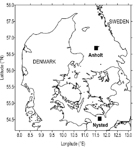
Fig. 2. Location of the sites at Anholt and Nysted in Denmark.
and Qiu, 1997) although errors in the derived humidity fluxes are relatively large in comparison with observations partic-ularly in stable conditions (Rutgersson et al., 2001; Strub and Powell, 1987). One well-known formulation (Beljaars et al., 1989) typically uses the measured temperature profile to determine the sensible heat flux and an iterative solution (Van Ulden and Holtslag, 1985) for the latent heat flux, the potential temperature scale (θ∗)and the humidity scale (q∗) based on a modified form of the Priestly and Taylor equation (Priestley and Taylor, 1972). This givesq∗as:
q∗=α
cp λ
s
(1+α)s+1θ∗ (11)
Wherecp is the specific heat capacity for dry air. λ is the latent heat of evaporation. s is the derivative of the water vapor saturation pressure as a function of temperature.αis a constant set to 0.128.
Once the humidity scaleq∗has been estimated it is used to calculate the virtual potential temperature:
θv∗=θ∗+0.61θ q∗ (12)
Which can then be used to determineLfrom Eq. (2). These bulk parameterizations were derived principally for use over land and, as can be seen from Eq. (11), the sign of
q∗is set via the sign ofθ∗i.e. ifθ∗is positiveq∗ is defined as positive. However the latent heat flux offshore is upward (Sempreviva and Hoejstrup, 1998) i.e.q∗is negative. The im-pact of humidity on the value of the Monin-Obukhov length,
L, is through the use ofθv∗rather thanθ∗in Eq. (2) and, in
stable conditions,Lis larger due to the presence of humidity fluxes. Note that the sign of the Monin-Obukhov length (pos-itive or negative) is dictated solely by the temperature flux. FromL, the stability parameter (z/L)is then determined and the wind speed profile calculated from the wind speed mea-sured at 10 m (or any other height) using Eq. (1).
2.3 Role of the boundary layer height
It has recently been suggested that for wind speeds above 50– 80 m from the surface, deviations from the wind profile based on surface-layer theory and Monin-Obukhov scaling increas-ingly occur, and at least in stable conditions these devia-tions are dependent on an additional length scale (the bound-ary layer height) (Gryning et al., 2007). This has prompted the suggestion that the surface-layer equations for the wind speed profile described in Eq. (1) should be modified in sta-ble conditions as follows (Gryning et al., 2007):
Uz=u∗
κ
lnz
z0
−9m z
L
1− z
2zi
(13) Wherezi is the boundary-layer height.
In the absence of specific measurements of the boundary-layer height,zi may estimated using (Gryning et al., 2007):
zi=0.12u∗
fc
(14) Wherefcis the Coriolis parameter.
Herein the relative impact of the humidity correction and the boundary layer height correction to wind speed profiles are compared.
3 Evidence for the importance of latent heat fluxes on the vertical wind profile
3.1 Data from the Anholt Experiment
Data presented here are derived from three intensive mea-surement campaigns over two week periods on the small Danish island of Anholt (Fig. 2) conducted between Septem-ber 1990 and OctoSeptem-ber 1992 (Sempreviva and Gryning, 1996). During the experiments, a 22 m meteorological mast was equipped with standard meteorological equipment in addi-tion to a 3-D sonic anemometer and a fast response hygrom-eter. The site was situated 10 m from the coast on the western part of the island giving an offshore fetch of at least 50 km from 240–360◦and a land fetch from 30–100◦.
The resulting data were conditionally sampled by wind di-rection into ‘land’ and “sea” fetches and used to compute the partitioning of the stability parameterz/Lbetween the con-tributions from sensible (z/LT)and latent heat fluxes (z/Lq)
Fig. 3. Partitioning ofz/Lbetweenz/LT andz/Lqfor land (left) and offshore (right) conditions using data from Sempreviva and Gryning
(1996). Over land the influence of humidity fluxes (z/Lq)is small andz/Lis dominated byz/LT. The horizontal axis indicates totalz/L
while the vertical axis shows values for bothz/LT andz/Lq.
conditions) indicate thatz/Lq can account for up to 30% of
the totalz/L.
The measurements from Anholt were used to quantify the magnitude of the effect of humidity fluxes on the stability correction to wind speed profiles. In this analysisLis cal-culated from the sonic anemometer temperature measure-ments using Eqs. (2–6) and the observed wind speed at 22 m height extrapolated to 150 m height using Eq. (1). This is approximately the tip height of current wind turbines being deployed offshore (2–3 MW range). In the first calculations, the Monin-Obukhov length is calculated using only sensible heat flux (i.e.z/L=z/LT)and in the second set of
calcula-tions the latent heat flux is included (i.e.z/L=z/LT+z/Lq)
(Fig. 4). In stable conditions, inclusion of humidity fluxes reduces the predicted wind speed at 150 m height by approx-imately 5% relative to a profile computed without their inclu-sion (Fig. 4). In unstable conditions, latent heat fluxes play a much smaller role in dictating the overall stability and hence there is a negligible effect on wind speed profiles. This is be-cause a change in the value ofLin unstable conditions due to humidity increases fluxes forcing conditions to be more unstable and, as shown in Eq. (6), the stability correction to the wind speed profile in unstable conditions tends to be smaller and much less sensitive to the value ofLthan in sta-ble conditions. Additionally the influence of humidity flux must be small unless the value of the sensible heat flux is small (Mahrt et al., 1998) and this is also consistent with the influence of humidity fluxes being important only in stable conditions.
Assuming thatz/Lneeds to be corrected to includez/Lq
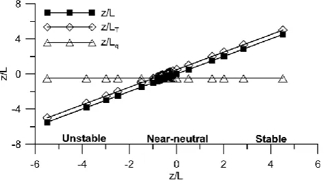
only in stable conditions, data from Anholt were used to de-rive an empirical correction toz/Las shown in Fig. 5. Here the ratio (z/L)/(z/LT)was compared withz/LT for
posi-Fig. 4. The influence of humidity fluxes on the wind profiles
us-ing data from the Anholt experiment (Sempreviva and Grynus-ing, 1996). The filled symbols are the normalized wind speed profile predicted using Eq. (1) and the experimentalz/Lincluding humid-ity fluxes; the open symbols are the wind speed profile without hu-midity fluxes. Inclusion of huhu-midity fluxes does not influence the profile for unstable conditions but in stable conditions the profile is driven towards neutral.
tive values ofz/Land an empirical relationship derived that can be used to estimatez/Lfor stable conditions offshore. The corrected wind speed profile calculated from the scaled
z/Lq is compared with alternative stability corrected wind
speed profiles below.
3.2 Data from the Nysted wind farm
[image:5.595.309.549.324.452.2]Fig. 5. The relationship betweenz/L,z/LT and z/Lq using data
from the Anholt experiment.
likely to be associated with substantial impact of humidity fluxes on the wind speed profile are observed, and to assess the degree to which inclusion ofLqin computingLimproves
the fit between the predicted and observed wind speed pro-files. Two years of relative humidity (RH) measurements at 10 m using a Vaisala HMP45A & HMP45D temperature and humidity sensor, wind speeds from 10, 25, 40, 55, 65 and 69 m collected using Risø RISØ P2546 cup anemome-ters (Pedersen, 2004), and temperature from Ametek pt-100 instruments at 10 and 65 m were used in the analysis. The RH measurements have an accuracy of 1%, and indicate rel-atively little seasonal variability, with monthly average RH varying between 79% and 87%.
Monin-Obukhov length computed from the temperature measurements at 65 and 10 m and the standard approach of (Beljaars et al., 1989) indicate about 33% of the observations are in the stable class with 0.05< z/L <1 (Fig. 6), implying that both the humidity correction and the boundary-layer cor-rection can be important influences on the wind speed profile because both apply under stable conditions. In the following,
Lwas recalculated using different methods to determineθv: – If no humidity measurements are available, q∗ can be estimated using procedure from Beljaars et al. (1989) as described in Sect. 2.2.2 except thatq∗is always nega-tive.
[image:6.595.309.546.63.241.2]– If RH is available, the specific humidityq, whereq is
Fig. 6. The frequency of stability class is calculated from
meteoro-logical data from the Nysted wind farm over the period June 2004– May 2006. As shown near-neutral conditions (abs(z/L) <0.05) are the most frequent, but slightly stable to stable (0.05< z/L <1) con-ditions account for about 33% of the observations.
the mass of water vapour per unit mass of air, including the water vapour can be calculated from:
q=εe(1−ε)
P (15)
Whereε is the ratio of gas constants for dry air to that of water vapour (0.622).
eis the vapor pressure of water vapor can be derived from the saturation vapor pressure calculated for the measured temperature (see e.g. Stull, 2000) and the relative humidity.
Assuming the surface layer at height 0 m is saturated with respect to water vapor givingq0,q∗can then be calculated as:
q∗=(q−q0)κ/
ln( z z0q
)−9H z
L
+9H zoq
L
(16)
Where the functions9H Lz
and9H zoq
L
are assumed to be the same as those for heat and roughness length for humidity,
z0q, is defined:
z0q=1.3×10⁻⁴+0.93×10⁻⁵/u∗ (17) Thus six methods were used to determine the wind profile up to 65 m for each 10-min wind speed measurement at 10-m:
1. Logarithmic: Where Eq. (1) is applied with the stability correction9m(z/L)set to 0.
Table 1. Predicted wind speeds at 69 m (from an initial height of 10 m a.m.s.l.) normalized by the observations for 2 years of 10-min data
from the Nysted wind farm. The wind speed predictions are made using 6 approaches: 1. Logarithmic: Where Eq. (1) is applied with the stability correction9m(z/L)set to 0.
2. Stability: Where Eq. (1) is applied with the stability correction9m(z/L)from the standard parameterization of Beljaars et al. (1989) except thatq∗is always negative.
3. Stability without humidity: Where Eq. (1) is applied with the stability correction9m(z/L)from the standard parameterization of Beljaars et al. (1989) but setting the latent heat flux to 0.
4. Stability with measured humidity: Where Eq. (1) is applied with the stability correction9m(z/L)applied using the parameterization from Beljaars et al. (1989) but withLqderived based on the observed relative humidity at 10 m as in Eqs. (15–17).
5. Stability with scaledz/Lin using the correction for stable cases from Eq. (18).
6. Stability with boundary layer (BL) correction: As 2) but using Eq. (13) for the wind speed profile in stable conditions.
The results are presented as the average in five stability classes defined on the basis ofz/L, and in terms of a mean of all data periods. Also shown is the Root Mean Square Error (RMSE) for all 65 m wind speed predictions from 10 m observations versus the observed wind speed at 65 m.
Stable Slightly Neutral Slightly Unstable Mean of RMSE stable unstable all data (m s−1) z/L 0.05< 0.01< |z/L|<0.01 −0.01< −1< z/L
z/L <1 z/L <0.05 z/L <−0.05 <−0.05 Ratio predicted/observed wind speed at 65 m height
1. Logarithmic 0.74 0.86 1.02 1.08 1.03 0.95 1.35 2. Stability 0.99 0.90 1.01 1.03 0.94 0.99 1.19 3. Stability without humidity 1.05 0.92 1.02 1.03 0.94 1.01 1.05 4. Stability with measured humidity 1.02 0.91 1.01 1.03 0.95 1.00 0.98 5. Stability with scaledz/L 0.94 0.90 1.01 1.03 0.94 0.95 1.09 6. Stability with boundary-layer correction 0.88 0.90 1.01 1.03 0.94 0.97 0.95
3. Stability without humidity: Where Eq. (1) is applied with the stability correction9m(z/L)applied using the standard parameterization from Beljaars et al. (1989) to computeLbut setting the latent heat flux to 0.
4. Stability with measured humidity: Where Eq. (1) is ap-plied with the stability correction9m(z/L)applied us-ing the parameterization from Beljaars et al. (1989) to computeLbut withLqderived based on the observed relative humidity at 10 m as in Eqs. (15–17).
5. Stability with scaledz/Lin using the correction for sta-ble cases given in Fig. 6 where:
z
L=0.115ln
z
LT
+0.848 (18)
6. Stability with boundary layer (BL) correction: As 2) but using Eq. (13) for the wind speed profile in stable con-ditions.
Note that in the first four methods, the value of z/L is changed by the selected parameterization but in methods 5 and 6 only the correction to the profile in stable conditions
is changed. The results are shown in Table 1 as the aver-age ratio of predicted to observed wind speeds at 65 m height for five stability classes. As in previous work (Motta et al., 2005), the use of the stability parameter improves the pre-diction of the mean wind speed compared to the logarithmic profile. Changes relating to the humidity flux determination (methods 2–4) have a relatively small impact on the mean wind speed profile. Methods 5 and 6 which impact the wind speed profile calculated in stable conditions have a larger im-pact on the overall wind speed profile because the corrections become relatively large. However, the root mean square error indicates that method 6 (stability with BL correction) gives the smallest error, while the results using measured relative humidity to derive the stability correction are overall slightly better than using the other stability methods. The scaled
z/Lqmethod gives a correction which is too large suggesting that the results from Anholt were not generalizable.
Fig. 7. Difference in predicted wind speeds at 150 m where
Udifferenceis defined as:
Udifference=100·(UC150−US150)/US150
WhereUS150 is the wind speed at 150 m extrapolated from 10 m
usingLcomputed using the Beljaars et al. (1989) bulk formula-tion and Eq. (1). AndUC150is the wind speed at 150 m calculated
as forUS150except (a) without humidity correction whereL
com-puted excludes the contribution fromLqor (b) with boundary layer
correction where the wind speed profile in stable conditions is de-termined from Eq. (13).
different humidity corrections are relatively small, the inclu-sion of the role of humidity fluxes does improve the wind speed predictions at 65 m. Excluding the standard latent heat flux correction as specified in Beljaars et al. (1989) gives the highest wind speed prediction at 65 m as expected. Addi-tion of the boundary layer height correcAddi-tion or the scaledz/L
tends to move the profile such that the extrapolated values are more negatively biased relative to the observations at 65 m. However, the overall RMSE is reduced. Although the re-sults are not conclusive the general indications from predict-ing wind speed profiles at Nysted appear to be; the stability correction to the wind speed profile is needed, the method of calculating the humidity correction is not important, and the scaledz/Land boundary layer correction both over-correct the wind speed profile in very stable conditions. Lack of in-formation regarding these influences adds to the uncertainty in the prediction of the wind speed profile.
3.3 Comparison of the size of the humidity and boundary-layer corrections
As mentioned above, wind turbine hub-heights for offshore deployment greatly exceed 65 m. Hence calculations were performed to examine the relative magnitude of the z/Lq
corrections considered herein on the vertical wind speed ex-trapolation from 10 m to 150 m. Wind speeds at 150 m height
were determined using Eqs. (1) and (2) with the standard hu-midity correction from Beljaars et al. (1989). Two correc-tions to this profile were then calculated i) computingLi.e. Eq. (2) without humidity fluxes and ii) the correction for the boundary layer height (Eq. 13). Wind speeds at 150 m were determined for a range ofz/Land the difference between the predicted wind speeds compared. As shown in Fig. 7, ex-cluding humidity fluxes makes a difference of up to 4% in the stable classes. For the boundary-layer correction, there is quite a wide range of wind speed predictions for simi-larz/L values using Eq. (13) because of the sensitivity of the boundary-layer correction to estimatedzi. At low wind
speeds,u∗is low,zi is small and the boundary-layer correc-tion becomes large. For moderately stable condicorrec-tions (where
z/L <0.1), the magnitude of the boundary-layer correction and the humidity correction are of similar magnitude (a few percent). Such conditions are frequently observed at least at the Nysted wind farm which implies the inclusion of la-tent heat fluxes in determiningLand corrections to the wind profile have a high degree of applicability to the wind energy industry. As conditions become increasingly stable, the mag-nitude of the boundary-layer correction increases and rapidly becomes very large, while the influence of latent heat fluxes declines.
4 Conclusions
As wind energy develops offshore and resource predictions are required for greater heights, better understanding of the wind speed profile over the sea is required. One of the major differences between on- and offshore is the constant pres-ence of strong (upward) latent heat fluxes offshore. In stable conditions, the sensible heat flux is downward and including the influence of latent heat fluxes reduces the stability (drives conditions towards neutral by reducingz/L)and the vertical wind shear. In unstable conditions, both latent and sensible heat fluxes are upwards and the inclusion of latent heat fluxes reinforces the instability but due to the relatively large sensi-ble heat flux and the moderate correction to the wind speed profile in unstable conditions, the effect on the vertical pro-file of wind speeds is minor.
Data from measurement campaigns at the island of An-holt in Denmark indicate that the contribution of humidity to fluxes offshore is up to about 30% in the stability pa-rameter the Monin-Obukhov length. A scaledz/Lderived from these data was evaluated against other methods of de-riving the humidity contribution using data from an offshore mast at the wind farm site at Nysted in Denmark. Inclu-sion of the humidity contribution to L has little influence on the average wind speed profile – the mean correction to the wind speed profile is relatively small (less than 2% at 65 m), but it does reduce the RMSE of the vertically extrap-olated wind speeds. Inclusion of humidity to calculation of
relatively insensitive to the precise mechanism used to com-puteq∗. Both the scaledz/Lapproach for humidity and a recently published correction for the height of the boundary layer over-correct the wind speed profile in very stable con-ditions and thus under-predict shear at the Nysted wind farm. Moderately stable conditions are frequently observed at offshore sites in northern Europe. Under these conditions the correction resulting from consideration of latent heat fluxes is of the same magnitude as the correction for boundary-layer height, and is worthy of consideration in vertical extrapola-tion of wind speeds in marine atmospheres. However it must be acknowledged that latent heat fluxes in the north of Eu-rope are relatively modest (Yu and Weller, 2007) and this is an indication that the latent heat correction to the stability pa-rameter could be larger, and hence more important, in other regions (Geernaert and Larsen, 1993).
Understanding the impact of humidity fluxes on wind speed profiles has relevance not only for accurate assessment of current wind energy resources and for the retrieval of wind speeds from satellite images (West and Yueh, 1996), but may also be of importance in considering how wind speed pro-files may change in areas which currently experience sea ice during winter but may become ice free under global climate change (Meier et al., 2004) thus changing the stability cli-mate.
Acknowledgements. This work has been funded in part by the
National Science Foundation projects (#0618364 and #0828655) and the EU Marie Curie Programme, Training Network activity, ModObs [MRTN-CT-19369] Network and by EU project UpWind #SES6 019945. We would like to acknowledge DONG Energy and Vattenfall for the use of the Nysted meteorological mast data.
Topical Editor F. D’Andrea thanks two anonymous referees for their help in evaluating this paper.
References
Barthelmie, R. J.: The effects of atmospheric stability on coastal wind climates, Meteorological Applications, 6, 39–48, 1999. Barthelmie, R. J.: Evaluating the impact of wind induced roughness
change and tidal range on extrapolation of offshore vertical wind speed profiles, Wind Energy, 4, 99–105, 2001.
Barthelmie, R. J., Pryor, S. C., and Frandsen, S. T.: Climatological and meteorological aspects of predicting offshore wind energy, in: Offshore wind energy, edited by: Twidell, J. and Gaudiosi, G., Multi-Science Publishing Co. Ltd, 2009.
Beljaars, A. C. M., Holtslag, A. A. M., and van Westrhenen, R. M.: Description of a software library for the calculation of surface fluxes., KNMI, De Bilt, Netherlands, 1989.
Capps, S. B. and Zender, C. S.: Global ocean wind power sensi-tivity to surface layer stability, Geophys. Res. Lett., 36, L09801, doi:10.1029/2008GL037063, 2009.
Charnock, H.: Wind stress on a water surface, Q. J. Roy. Meteorol. Soc., 81, 639–640, 1955.
Cleve, J., Grenier, M., Enevoldsen, P., Birkemose, B., and Jensen, L.: Model-based analysis of wake-flow data in the
Nysted offshore wind farm, Wind Energy, 12(2), 125–135, doi:10.1002/we.314, 2009.
Danish Energy Authority: Future Offshore Wind Power Sites -2025. Danish Energy Agency. The Committee for Fu-ture Offshore Wind Power Sites, April 2007, Copenhagen, http://193.88.185.141/Graphics/Publikationer/Havvindmoeller/ Fremtidens 20havvindm UKsummery aug07.pdf, 2007. de Vries, E.: 40,000 MW by 2020: Building offshore wind in
Eu-rope, Renewable Energy World, 11(1), 36–47, 2008.
de Vries, E.: Optimism in Offshore Wind, Renewable Energy World, 12(6), 27–37, 2009.
Frank, H. P., Larsen, S., and Højstrup, J.: Simulated wind power offshore using different parameterizations for the sea surface roughness, Wind Energy, 3, 67–79, 2000.
Geernaert, G. and Larsen, S.: On the role of humidity in estimating marine surface layer stratification and scatterometer cross sec-tion., J. Geophys. Res., 98, 927–932, 1993.
Gryning, S. E., Batchvarova, E., Br¨ummer, B., Jørgensen, H. E., and Larsen, S. E.: On the extension of the wind profile over homo-geneous terrain beyond the surface boundary layer, Bound.-Lay. Meteorol., 124, 251–268, 2007.
GWEC: No slow-down for global wind energy, Global Wind En-ergy Council, http://www.gwec.net/, accessed 20 April 2010. Holtslag, A. A. M.: Estimates of diabatic wind speed profiles from
near-surface weather observations., Bound.-Lay. Meteorol., 29, 225–250, 1984.
IEA: IEA Wind Energy Annual Report 2007, http://www.ieawind. org/AnnualReports PDF/2007/200720IEA20Wind20AR.pdf, 2008.
Large, W. G. and Pond, S.: Sensible and latent heat flux measure-ments over the ocean, J. Phys. Ocenaogr., 12, 464–482, 1982. Mahrt, L., Vickers, D., Edson, J., Sun, J., Hojstrup, J., Hare, J., and
Wilczak, J.: Heat flux in the coastal zone, Bound. Lay. Meteorol., 86, 421–446, 1998.
Meier, H. E. M., Doescher, R., and Halkka, A.: Simulated distribu-tions of Baltic sea-ice in warming climate and consequences for the winter habitat of the Baltic ringed seal., Ambio, 33, 249–256, 2004.
Motta, M., Barthelmie, R. J., and Vølund, P.: The influence of non-logarithmic wind speed profiles on potential power output at Danish offshore sites., Wind Energy, 8, 219–236, 2005. Musial, W.: Offshore wind electricity: A viable energy option for
the coastal united states, Mar. Technol. Soc. J., 41, 32–43, 2007. Pedersen, T. F.: Characterisation and Classification of RISØ P2546 Cup Anemometer. Risoe National Laboratory, Roskilde, http:// www.risoe.dk/rispubl/VEA/veapdf/ris-r-1364 ed2.pdf, 2004. Pe˜na, A., Gryning, S. E., and Hasager, C. B.: Measurements and
modelling of the wind speed profile in the marine atmospheric boundary layer, Bound.-Lay. Meteorol., 129, 479–495, 2008. Priestley, C. H. B. and Taylor, R. J.: On the assessment of
sur-face heat flux and evaporation using large scale parameters, Mon. Weather Rev., 106, 81–92, 1972.
Ruprecht, E. and Simmer, C.: Fluxes of latent heat over the oceans: climatological studies and application of satellite observations, Dyn. Atmos. Oceans, 16, 111–121, 1991.
Rutgersson, A., Smedman, A., and Omstedt, A.: Measured and sim-ulated latent and sensible heat fluxes at two marine sites in the Baltic Sea, Bound.-Lay. Meteorol., 99, 53–84, 2001.
marine boundary layer measured at a coastal site with an infrared humidity sensor, Bound.-Lay. Meteorol., 77, 331–352, 1996. Sempreviva, A. M. and Hoejstrup, J.: Transport of temperature and
humidity variance and covariance in the marine surface layer, Bound.-Lay. Meteorol., 87, 233–253, 1998.
Sempreviva, A. M., Larsen, S. E., Mortensen, N. G., and Troen, I.: Response of neutral boundary layers to changes of roughness, Bound.-Lay. Meteorol., 50, 205–226, 1990.
Simpson, J. E.: Sea breeze and local winds, Cambridge University Press, Cambridge, 1994.
Smedman, A., Hogstrom, U., Bergstrom, H., Rutgersson, A., Kahma, K., and Petterson, H.: A case study of air-sea interaction during swell conditions, J. Geophys. Res., 104, 25833–25851, 1999.
Smedman, A. S., Hogstrom, U., and Bergstrom, H.: Low level jets – a decisive factor for off-shore wind energy siting in the Baltic Sea, Wind Engineering, 20, 137–147, 1996.
Strub, P. T. and Powell, T. M.: The exchange coefficients for latent and sensible heat flux over lakes: dependence upon atmospheric stability, Bound.-Lay. Meterol., 40, 349–361, 1987.
Stull, R. B.: An introduction to boundary layer meteorology, Kluwer Publications Ltd, Dordrecht, 1988.
Stull, R. B.: Meteorology for scientists and engineers, Brooks/Cole, Pacific Grove, CA, 2000.
Subrahamanyam, D. B., Rani, R. I., Ramanchandran, R., Kun-hikrishnan, P. K., and Kumar, B. P.: Impact of wind speed and atmospheric stabiity of air-sea interface fluxes over the east Asian Marginal Seas, Atmos. Res., 94(1), 81–90, doi:10.1016/j.atmosres.2008.09.11, 2009.
Tambke, J., Lange, M., Focken, U., Wolff, J., and Bye, J.: Forecast-ing offshore wind speeds above the North Sea, Wind Energy, 8, 3–16, 2005.
Van Ulden, A. P. and Holtslag, A. A. M.: Estimation of atmospheric boundary layer parameters for diffusion applications., J. Clim. Appl. Meteorol., 24, 1196–1207, 1985.
Wenzel, A. and Kalthoff, N.: Method for calculating the whole-area distribution of sensible and latent heat fluxes based on climato-logical observations, Theor. Appl. Climatol., 66, 139–160, 2000. West, R. D. and Yueh, S. H.: Atmospheric effects on the wind re-trieval performance of satelliteradiometers. Geoscience and Re-mote Sensing Symposium, ReRe-mote Sensing for a Sustainable Fu-ture, 27–31 May 1996.
Xu, Q. and Qiu, C.-J.: A Variational Method for Computing Surface Heat Fluxes from ARM Surface Energy and Radiation Balance Systems, J. Appl. Meteorol., 36, 3–11, 1997.