https://doi.org/10.5194/gmd-11-1577-2018 © Author(s) 2018. This work is distributed under the Creative Commons Attribution 4.0 License.
On the effect of model parameters on forecast objects
Caren Marzban1,2, Corinne Jones2, Ning Li2, and Scott Sandgathe1 1Applied Physics Laboratory, Univ. of Washington, Seattle, WA 98195 USA 2Department of Statistics, Univ. of Washington, Seattle, WA 98195 USA
Correspondence:Caren Marzban ([email protected]) Received: 1 November 2017 – Discussion started: 13 November 2017
Revised: 8 February 2018 – Accepted: 22 March 2018 – Published: 19 April 2018
Abstract.Many physics-based numerical models produce a gridded, spatial field of forecasts, e.g., a temperature “map”. The field for some quantities generally consists of spatially coherent and disconnected “objects”. Such objects arise in many problems, including precipitation forecasts in atmo-spheric models, eddy currents in ocean models, and models of forest fires. Certain features of these objects (e.g., location, size, intensity, and shape) are generally of interest. Here, a methodology is developed for assessing the impact of model parameters on the features of forecast objects. The main in-gredients of the methodology include the use of (1) Latin hypercube sampling for varying the values of the model pa-rameters, (2) statistical clustering algorithms for identify-ing objects, (3) multivariate multiple regression for assessidentify-ing the impact of multiple model parameters on the distribution (across the forecast domain) of object features, and (4) meth-ods for reducing the number of hypothesis tests and control-ling the resulting errors. The final “output” of the method-ology is a series of box plots and confidence intervals that visually display the sensitivities. The methodology is demon-strated on precipitation forecasts from a mesoscale numerical weather prediction model.
Copyright statement. The author’s copyright for this publication is transferred to the University of Washington.
1 Introduction
Complex, physics-based numerical models of natural phe-nomena often have parameters – henceforth, model param-eters – whose values are generally not a priori specified. In such situations it is important to infer the manner in which
the model parameters affect the outputs of the model (i.e., forecasts or predictions), and often the techniques of sen-sitivity analysis (SA) are employed to assess the effects. There is a wide range of techniques from a relatively simple one-at-a-time method (also known as the Morris method) in which each model parameter is varied individually (e.g., Yu et al., 2013) to multivariate approaches motivated by statisti-cal methods of experimental design (Montgomery, 2009) in which the values of the model parameters are varied accord-ing to some optimization criterion. Alternative approaches can be found in Backman et al. (2017) in which algorithmic differentiation is used and in Kalra et al. (2017) in which the underlying physics equations are integrated using quadrature methods. And yet another alternative is the adjoint method commonly used in meteorological circles (Errico, 1997).
It is difficult to classify the various methods into a simple taxonomy (Bolado-Lavin and Badea, 2008), but the terms lo-cal and global have been used to denote two broad categories (Saltelli et al., 2010, 2008); generally, local methods employ some sort of derivative of the model output with respect to in-puts, while global techniques rely on a decomposition of the variance of the output in terms of the variance explained by the inputs. Comparisons of the various approaches are not commonplace because each approach is usually suited for a specific application for which other methods may not be practically feasible. However, an example of the comparison of one global approach and one local (adjoint) approach on the Lorenz ’63 model (Lorenz, 1963) has been performed by Marzban (2013).
pa-rameters on the probability of model crashes. By contrast, sometimes SA is performed as an intermediate step to an-other goal, such as the calibration of the model (Safta et al., 2015; Hacker et al., 2011; Laine et al., 2012; Ollinaho et al., 2014). All of these classification criteria are imperfect, as there are works that fall “between” global versus local or SA-only versus SA-for-calibration; some examples include Roebber (1989), Roebber and Bosart (1989), and Robock et al. (2003). The work reported here falls into the local and SA-only category; as such, although the proposed methodol-ogy can be used for calibration, no attempt is made to do so here.
In many SA studies, the output of the model (i.e., the re-sponse variable in the SA) is usually a single or a handful of scalar quantities. But there are situations in which the output is a gridded spatial field, e.g., temperature forecasts over a spatial region. Every grid point reflects a forecast at that lo-cation, and for a quantity like temperature the field as a whole has a smooth, continuous nature. SA is more complicated for precipitation fields in which the model output is a quantity whose spatial structure is not smooth and/or continuous. In-deed, there may be a coherent set of grid points that receive no precipitation at all, while an adjacent set of grid points will reflect a complex pattern of precipitation. In short, the spatial field of such quantities will contain “objects” within which precipitation does occur surrounded by regions of lit-tle or no precipitation. Such objects arise in a wide range of Earth systems, e.g., models of ocean currents and eddies (e.g., Fig. 1 in Samsel et al., 2015), atmospheric plume and dispersion (e.g., Fig. 4 in Stein et al., 2015), ocean garbage transport (e.g., Fig. 2 in Froyland et al., 2014), forest fires (e.g., Fig. 8 in Vogelmann et al., 2011), and models of the Earth’s mantle (e.g., Fig. 4 in French et al., 2013).
For such discrete fields, the assessment of the quality of the forecasts has given rise to a wide range of specialized techniques generally referred to as spatial verification (or evaluation) (Ahijevych et al., 2009; Baldwin et al., 2001, 2002; Brown et al., 2002; Casati et al., 2004; Davis et al., 2006a, b; Du and Mullen, 2000; Ebert, 2008; Ebert and McBride, 2000; Gilleland et al., 2009; Hoffman et al., 1995; Keil and Craig, 2007; Marzban and Sandgathe, 2006, 2008; Marzban et al., 2008, 2009; Nachamkin, 2004; Roberts and Lean, 2008; Wealands et al., 2005; Wernli et al., 2008; Venu-gopal et al., 2005; Li et al., 2015). A subset of these methods employs the notion of an object explicitly. In some applica-tions, the object is defined subjectively, for example by ex-perts. In other applications statistical methods for clustering (Everitt, 1980) are used to identify and define objects within the field (Marzban and Sandgathe, 2006, 2008). This cluster-ing approach, which has been reexamined by Lakshmanan and Kain (2010) and more recently by Wang et al. (2015), is the basis of the object-identification procedure used in the present work.
Although no spatial verification or evaluation is done here, the importance of objects within the forecast field calls for
an SA framework wherein one can assess the effect of model parameters on features of the objects. Also, the assessment of sensitivity is highly intertwined with that of statistical sig-nificance. The methodology developed here can be viewed as an object-based SA with which one can assess the impact (both the magnitude and the statistical significance) of model parameters on object features.
More specifically, the next section describes the main components of the proposed methodology, namely Latin hy-percube sampling for determining how the model parameters are varied (Sect. 2.1) and the use of clustering algorithms for identifying objects in the forecast field (Sect. 2.2). The object features examined here, generally of interest in many applications, include size, location, intensity, and shape, all of which can be readily estimated from the forecasts directly (Sect. 2.3). Section 2.4 describes multivariate multiple re-gression for assessing the impact of the model parameters on the distribution (across the forecast domain) of object fea-tures. Anticipating the problems associated with multiple hy-pothesis testing, steps are taken to first reduce the number of tests and then to control different error rates (Sect. 2.5). Ultimately box plots and confidence intervals are used to vi-sually display the daily variability of the sensitivities. Sec-tion 2.6 summarizes all of these components and is followed by a demonstration of the methodology on forecasts from a weather prediction model (Sect. 3). The paper ends with a statement of the conclusions, additional discussion, and ways in which the methodology can be generalized (Sect. 4).
2 Method 2.1 Data
The numerical model employed to demonstrate the method-ology is COAMPS®(Hodur, 1997), for which some SA work has already been done. Doyle et al. (2011) and Jiang and Doyle (2009) examine the effect of model parameters on mountain waves. Motivated by the work of Holt et al. (2011), who studied the effect of 11 model parameters on various characteristics of the forecasts, Marzban et al. (2014) used a global, variance-based SA to study the effect of the same pa-rameters and their interactions on the mean (across the fore-cast domain) and the center-of-gravity of precipitation. By contrast, here the effect of the model parameters is assessed on features of objects within the forecast field. As discussed in Sect. 2.3, a total of six features are examined, together summarizing the location, intensity, and the shape of each object.
These 11 parameters are the inputs to the numerical model, and the outputs are forecasts of precipitation at each of 45
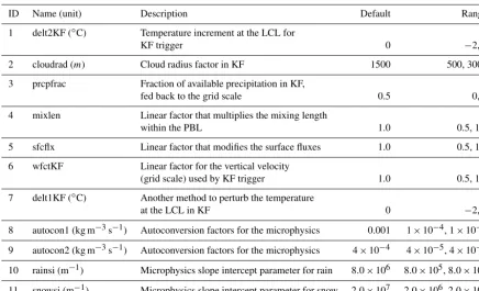
Table 1.The 11 parameters studied in this paper. Also shown are the default values and the range over which they are varied.
ID Name (unit) Description Default Range
1 delt2KF (◦C) Temperature increment at the LCL for
KF trigger 0 −2, 2
2 cloudrad (m) Cloud radius factor in KF 1500 500, 3000
3 prcpfrac Fraction of available precipitation in KF,
fed back to the grid scale 0.5 0, 1
4 mixlen Linear factor that multiplies the mixing length
within the PBL 1.0 0.5, 1.5
5 sfcflx Linear factor that modifies the surface fluxes 1.0 0.5, 1.5
6 wfctKF Linear factor for the vertical velocity
(grid scale) used by KF trigger 1.0 0.5, 1.5
7 delt1KF (◦C) Another method to perturb the temperature
at the LCL in KF 0 −2, 2
8 autocon1 (kg m−3s−1) Autoconversion factors for the microphysics 0.001 1×10⁻⁴, 1×10⁻²
9 autocon2 (kg m−3s−1) Autoconversion factors for the microphysics 4×10⁻⁴ 4×10⁻⁵, 4×10⁻³
10 rainsi (m−1) Microphysics slope intercept parameter for rain 8.0×10⁶ 8.0×10⁵, 8.0×10⁷ 11 snowsi (m−1) Microphysics slope intercept parameter for snow 2.0×10⁷ 2.0×10⁶, 2.0×10⁸
KF: Kain–Fritsch, PBL: planetary boundary layer, LCL: lifted condensation level
by generating an ensemble (or sample) of input values, as-similating surface observations, and then running the model forward to produce 24 h forecasts of precipitation amount at each grid point. As such, the SA results are contingent on the nature of these data, and consequently care must be taken in the data-generation step of the methodology.
The data used for the SA must be representative of the range of the phenomena observed at large. To that end, the present application involves a wide range of weather phenomena spanning 120 days from 16 February through 2 July 2009. Confirmed by visual examination of all 120 forecasts, this temporal period includes a comprehensive series of midaltitude synoptic systems traveling across the northern portion of the domain. These synoptic systems ex-tend down into the southeastern US early in the period and are replaced by subtropical convective systems in the late spring and summer months. This subtropical activity also oc-curs in the southwestern portion of the domain (west coast of Mexico) during June and July in association with the south-west monsoon. The only apparent atypical weather appears to be a greater amount of convective activity off the east coast of the US associated with quasi-stationary or slow-moving frontal systems during the period.
It is important that the data cases are as independent as possible. To that end, the 120 days are sampled at 3-day in-tervals in order to minimize temporal dependency, leading to 40 days for the analysis.
For each of the 40 days, 99 different values for 11 parame-ters are generated by Latin hypercube sampling (LHS). Said differently, for each day, a sample of size 99 is taken from the 11-D space of the model parameters. This so-called “space-filling” sampling scheme ensures that no 2 of the 99 points have the same value for any of the 11 parameters. It can be shown that this property leads to more precise estimates (at least, no less-precise estimates) than many other sam-pling schemes (Cioppa and Lucas, 2007; Montgomery, 2009; Marzban, 2013). LHS is appropriate when the model param-eters are all continuous quantities (i.e., taking values on the real line). For discrete or categorical inputs, Latin square de-signs or fractional factorial dede-signs can be employed to pro-duce optimal samples (Montgomery, 2009); these methods will be demonstrated in a separate article.
Given that daily variability is a common source of variabil-ity in models dealing with Earth systems, one question that arises is whether one should use a given LHS sample for all days in the analysis. Here, in order to explore a larger portion of the model parameter space, the LHS sample is allowed to vary across each of the 40 days in the study. Although this choice confounds variability due to model parameters with daily variability, it is arguably a better choice than the alter-native (of using the same LHS sample across all days) be-cause the final sensitivity results will not be contingent on a given LHS sample.
mentioned in that paper, these parameters were chosen for their anticipated sensitivity (through model tests and discus-sions with developers) of the parameterizations in an effort to choose parameters most likely to produce changes in the model output precipitation fields. Also, to focus on heavy precipitation, only the grid points whose convective precip-itation amount exceeds the 90th percentile of precipprecip-itation across the domain are analyzed.
2.2 Cluster analysis
There is a wide range of clustering methods, each with their respective parameters (Everitt, 1980). At one extreme, there is a class of clustering methods wherein the desired number of clusters, NC, is specified by the user. A proven example in this class is called Gaussian mixture model (GMM) cluster-ing (McLachlan and Peel, 2000). At the other extreme, there are clustering routines in which NC does not play a role at all. One such method is called density-based spatial clustering of applications with noise (DBSCAN) (Ester et al., 1996). DB-SCAN has two parameters, here denotedand min_samples. Roughly speaking,is the maximum distance between two grid points in order for them to be in the same cluster, and min_samples is the minimum number of grid points neces-sary to form a cluster.
Here, these two approaches are selected for demonstration because they allow for two very different ways in which a user can inject a priori knowledge into the analysis. For ex-ample, in some applications it may be more natural to spec-ify the number of clusters, in which case GMM is a natural choice. On the other hand, DBSCAN is more natural if the user has knowledge of the typical size and distance between clusters. For example, consider a situation wherein the grid spacing is relatively large (as is the case in this paper, i.e., 81 km), allowing one to examine only large-scale precipita-tion. Although time of year and location are also important, if one were to focus only on winter months in, say, the Pacific Northwest, then it is reasonable to setto 3 or 4. By contrast, if one is considering jet streaks, e.g., where some maximum wind speed value is reached, then can be closer to 1. As for min_samples, 4 or 5 is a reasonable value for both pre-cipitation and jet streak events at the model resolution used here.
In addition to the way in which the respective parameters are handled, another reason why these two clustering meth-ods are used here is that they occupy two other extremes in the family of clustering algorithms: GMM clustering belongs to a class of model-based algorithms (Banfield and Raftery, 1993; Fraley and Raftery, 2002) common in statistics circles because they are conducive to performing statistical tests, while DBSCAN assumes no underlying model and for this reason is often employed in machine learning applications.
For the SA component of the methodology developed here, it is not necessary for the objects to be defined by these or any other clustering algorithm; the objects may be defined
by any other criterion or even by experts. But some gen-eral guidance on the available options may be in order. As mentioned previously, some algorithms require the specifica-tion of the number of clusters (e.g., GMM), while others re-quire information on the desired size and/or distance between clusters (e.g., DBSCAN). There is another class of cluster-ing algorithms wherein no such specification is required; an example of this type is hierarchical agglomerative cluster-ing (Everitt, 1980), wherein the procedure begins by assign-ing each ofN points to a unique cluster and then proceeds by combining the clusters systematically until all points are members of a single cluster. As such, this algorithm allows the number of clusters to vary systematically fromN to 1. A variation on this routine involves the reverse procedure wherein the number of clusters is varied from 1 toN. The clustering results may depend on the choice of these proce-dures, and so for any specific problem some trial-and-error experimentation is recommended.
In clustering algorithms that rely on a notion of distance, there are two types of distance that must be distinguished, generally referred to as intra-cluster and inter-cluster. The former refers to the distance between any two points, while the latter gauges the “distance” or similarity between two clusters. On gridded fields, the notion of an intra-cluster distance is itself ambiguous; two common choices are the Euclidean distance (defined by the Pythagorean theorem) and the Manhattan distance (defined by the sum of the grid lengths connecting two grid points). Although the resulting clusters do depend on the choice of this distance measure, the former generally lead to smaller and more distant clus-ters. Here, in DBSCAN, the Euclidean intra-cluster distance is used; GMM does not involve the notion of an intra-cluster distance.
In clustering algorithms that involve the notion of an inter-cluster distance, some consideration must be given to at least three common measures: (1) the group average distance (de-fined as the average of the intra-cluster distances between all the points across two clusters), (2) the distance between the closest grid points across the two clusters, and (3) the dis-tance between the farthest grid points across the clusters. The last two options are often called SLINK (for shortest or single link) and CLINK (for complete link), respectively. Again, the final clustering results may depend on the choice of this dis-tance, but CLINK generally results in tightly packed, small clusters. By contrast, SLINK leads to long and thin ters. A comparison of these distance measures in the clus-tering of precipitation forecasts is performed in Marzban and Sandgathe (2006). GMM and DBSCAN do not employ a no-tion of inter-cluster distance.
de-pending on the specific application. Although there are statis-tical criteria that lead to unique values for the parameters, the criteria involve the optimization of some other quantity, e.g., Akaike information criterion (AIC) or Bayesian information criterion (BIC). As such, the ambiguity in the choice of the clustering algorithm or the values of their parameters is sim-ply replaced with the ambiguity of selecting the appropriate criterion. Therefore, again, no attempt is made to optimize the values of the parameters. It is assumed that the user has sufficient information about the underlying physics to either specify the number of physical objects (or a range thereof) or the typical size and distance between physical objects.
2.3 Cluster features
In spatial verification some of the errors that are of interest include displacement, intensity, size and area, and shape er-ror. The estimation of these errors presumes the ability to compute the location, intensity, area, and shape of a cluster, respectively. Here, the latitude and longitude of the centroid of a cluster are taken as coordinates of its location, intensity is measured by the median (across the spatial extent of the cluster) of precipitation, and area is measured by the number of grid points in a cluster. The shape of a cluster in GMM is an ellipse because that is the cross section (i.e., level set) of a bivariate Gaussian. Then, the eccentricity and orientation of the semi-major axis of the ellipse are natural for quantifying the shape of clusters. In DBSCAN, clusters are not restricted to have any specific shape. In order to be able to compare the two clustering algorithms, here an elliptical shape is as-sumed for the clusters, and the eccentricity and orientation are obtained from the first and second eigenvectors of the covariance matrix computed from the coordinates of all the grid points in a given cluster. The length of the semi-major axis is set to the largest eigenvalue. The ability to estimate the shape of the ellipse from the covariance matrix is an im-portant component of the methodology because the alterna-tive of fitting curves through the edges of clusters is a much more complicated task. This covariance matrix is central to the construction of many other features of potential interest (Bookstein, 1991).
In short, the six cluster features examined here are latitude, longitude, intensity, area, orientation, and eccentricity. It is worth reiterating that these quantities can be estimated from the forecast field directly without any further modeling of the objects. Also, as explained in the next section, in order to assess how the distribution (across the forecast field) of a given feature is affected by the model parameters, the former is summarized with three moments: minimum, median, and maximum.
2.4 Statistical model
The SA methodology in Marzban et al. (2014) is a variance-based approach that allows one to identify linear or nonlinear
relationships between the forecast quantities and the model parameters and even interactions between the model param-eters. As a first approximation, however, it is sufficient to estimate only the linear (i.e., main) effects because nonlin-ear and interaction effects are often much smaller than main effects; see, for example, pages 192, 230, 272, 314, and 329 in Montgomery (2009) and pages 33–34 in Li et al. (2006). For this reason a linear regression-based model is adequate. Specifically, the effect of the model parameters is assessed via the least-squares estimate of the regression coefficients βi in
y=α+β1x1+β2x2+. . .+β11x11+δ , (1) wherexi denotes standardized model parameters,yis some
cluster feature, andδ represents any source of variability in yother than from the model parameters. This linear model is further justified by the results (shown below) because when it is specialized to the case of one cluster (i.e., the entire spa-tial domain), it reproduces the results of the variance-based approach reported in Marzban et al. (2014).
There is a realization of Eq. (1) in which the response is vector valued; the model is called multivariate multiple re-gression (MMR), wherein Eq. (1) is understood as a vector equation in whichy,α, and βi are all vectors (Fox et al.,
2013; DelSole and Yang, 2011; Rencher and Christensen, 2012). Ideally one could allow each component of the re-sponse vector to represent a forecast feature of a given object. However, the number of objects and clusters varies across the 99 values of the parameters and across days in the data. Methods for estimating MMR coefficients when the num-ber of responses is a random variable (varying across cases) are not readily available. Therefore, for each of the six fea-tures measuring location, intensity, and shape, three sum-mary measures are considered: the minimum, median, and maximum (across the clusters in the domain) of the feature. These three quantities can be thought of as a 3-point sum-mary of the distribution (technically, histogram) of the fea-ture, and they serve as the three responses in MMR. In short, the statistical model used here is
ydmin ymedd ymaxd
=
αmind αdmed αdmax
+
β1min,d β1med,d β1max,d
x1,d (2)
+
β2min,d β2med,d β2max,d
x2,d+ · · · +
β11min,d β11med,d β11max,d
x11,d (3)
+
δdmin δdmed δdmax
, (4)
where min, med, and max denote the minimum, me-dian, and maximum (across clusters), respectively, andd=
been suppressed. As mentioned previously, the 99 samples of the 11 model parameters are allowed to vary across the 40 days – hence thedsubscript on thexvariables in Eq. (2). In addition to serving as a 3-point summary of the dis-tribution of features, the minimum, median, and maximum also serve another purpose; the median is useful because one can assess the effect of the model parameters on a “typical” cluster, and the minimum and maximum across clusters are useful because they allow one to assess whether a model pa-rameter has an effect on any of the clusters in a field. For example, if it is found that a particular model parameter is positively (negatively) associated with the minimum (max-imum) size across clusters, then one can conclude that the size of at least one of the clusters in the field is affected by that parameter. This is an important consideration because if the size of at least one of the clusters is not affected by a pa-rameter, then that parameter can be said to have no effect on the size of clusters.
One may wonder why it is important to use MMR with three responses as opposed to three single-response multiple regression models; it is easy to show that the latter ignores the correlation between the response variables (Fox et al., 2013; Rencher and Christensen, 2012). As such, MMR pro-vides a better model of the underlying relationship between the model parameters and the response variables.
The data on the response variablesy are log transformed to assure more bell-shaped histograms; this transformation is not necessary, but is useful when the regression coefficients are subjected to statistical tests because many such tests as-sume relatively bell-shaped distributions.
2.5 Significance tests
Testing the coefficients in the MMR model involves perform-ing a large number of statistical tests(40×11×6×3): one on each of 40 days, for each of 11 parameters, for each of six cluster features, and for each of three summary measures across clusters. A large number of tests, in turn, leads to an exponential growth in the probability of making some Type I error. In general, the increase in the probability of making er-rors associated with multiple tests is known as the multiple hypothesis testing problem (Benjamini and Hochberg, 1995; Bretz et al., 2001; Dmitrienko et al., 2009; Montgomery, 2009; Rosenblatt, 2013; Wilks, 2011). There are several pro-cedures for addressing this problem, and they all involve two ingredients: (1) a set of “raw”pvalues resulting from multi-ple hypothesis tests and (2) the specification of an error rate to be controlled. Then, the p values are corrected (usually scaled) in order to control the error rate. Two common mea-sures of error rate are the family-wise error rate (FWER), defined as the probability of at least one Type I error, and the false discovery rate (FDR), which is the expected proportion of Type I errors among all the tests that lead to the rejec-tion of the null hypothesis. One of the simplest procedures for correcting thepvalues involves simply multiplying all of
thepvalues by the number of tests and then comparing these correctedpvalues with a fixed significance level (e.g., 0.05). This correction controls the FWER and is called the Bonfer-roni correction (Bretz et al., 2001; Wilks, 2011). One of the popular procedures for controlling the FDR, as introduced in Benjamini and Hochberg (1995), similarly involves scaling eachp value but by a quantity that depends on the rank of thepvalue. The choice of the error rate to be controlled is sometimes evident from the nature of the problem (Rosen-blatt, 2013), but not in the present case; for this reason, both corrections are examined.
Quite independently of the above methods for controlling the errors arising from the multiplicity of tests, there is a pro-cedure that is often practiced when one is faced with multiple hypothesis tests. The main goal of the procedure is to reduce the number of tests performed, and it is generally possible to do so in tests that involve linear models (Montgomery, 2009). In the first stage of the procedure, one performs a sin-gle, often-called omnibus, hypothesis test of whether any of the predictors (here, model parameters) in the linear model have an effect on any of the responses. If the null hypothesis cannot be rejected, then no more tests are performed, and the conclusion of the analysis is that there is no evidence that any of the parameters have an effect on any of the responses. If, however, the null hypothesis is rejected, then, and only then, one proceeds to the second stage of testing the significance of each of the parameters separately.
In the present application, the omnibus test used in the first stage is called the Pillai’s trace test (Fox et al., 2013; Rencher and Christensen, 2012), and its use reduces the total number of tests from 40×11×6×3 to only 40×6. Here, both FWER-and FDR-controlling corrections to thesepvalues are exam-ined. The second stage of the aforementioned procedure calls for testing the effect of each of the model parameters sepa-rately, but only for those comparisons that have been found significant in the first stage. However, here for the this sec-ond stage, no hypothesis testing is performed at all because in spite of the plethora ofpvalues they provide no information on the magnitude of the effect of each parameter. Instead, in the second stage, we examine the box plot of the estimated regression coefficients and the associated confidence inter-vals.
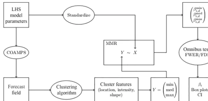
Figure 1.The flowchart highlighting the main components of the methodology.
the response in question. In such a case, the “distance” of the box plot relative to zero provides a visual indication of the magnitude of the effect.
The confidence interval for the mean (across 40 days) of the regression coefficient is computed from the estimates of the daily regression coefficients and their standard errors, all computed within MMR. Given that each of the aforemen-tioned displays in the final “output” of the methodology in-volves 11 CIs, a Bonferroni correction is introduced in order to ensure that FWER is maintained at 5 %. The interpretation of the CIs is similar to that of the box plots. If a CI excludes the number zero, one can reject the null hypothesis of no ef-fect with (at least) 95 % confidence; otherwise, there is no evidence to draw any conclusion. The overall position of the CI conveys information on the magnitude of the effect.
A brief discussion of the advantages and disadvantages of the box plot and the confidence interval (CI) is in order. The box plot can be considered to provide a 5-point summary of the empirical sampling distribution of a regression coef-ficient. The sampling distribution is more fundamental than the CI (and the p value) in the sense that the latter is de-rived from the former, and as such, the sampling distribution contains more information. However, this additional infor-mation comes at the cost of less rigor because hypothesis testing with box plots is inherently qualitative. CIs introduce a more rigorous display, but they too have some limitations. For example, whereas hypothesis testing with box plots does not require a notion of a confidence level, CIs depend ex-plicitly on that notion. Furthermore, analysis of multiple CIs suffers from the same problems that arise in multiple hypoth-esis testing withpvalues (see Sect. 2.5). Another limitation of CIs is that they are generally symmetric and so do not convey information on the shape (e.g., skew) of the under-lying distribution – box plots do; see the Discussion section for other alternatives. Given the different trade-offs between box plots and CIs, both are used here. Consequently, the fi-nal output of the methodology will consist of a figure
involv-ing 11 box plots and CIs (one per model parameter) for each of six forecast features and three summary measures (mini-mum, median, maximum) thereof.
2.6 Summary of method
This subsection summarizes the main ingredients of the pro-posed methodology and the associated problems (and solu-tions) that arise in an object-based SA. See the flowchart in Fig. 1.
In SA, when the model parameters are continuous, a com-mon method for varying them is LHS. It is important to point out that in models wherein daily variability is present, it is advisable to allow the LHS to vary across days.
The model, here COAMPS, is then run for each of the model parameter values in the LHS, and each of the gener-ated forecast fields is subjected to cluster analysis for the pur-pose of identifying objects in the forecast fields. The choice of the clustering algorithm is an important consideration. Some users may wish to use algorithms in which the number of objects is specified, while others may find it more natural to specify the typical size and/or distance between objects. GMM and DBSCAN are examples from each category. Yet other users may wish to examine all possible clusterings of a field, in which case a hierarchical method is more advisable. After the objects have been identified, one must decide what object features are of interest. Features that can be esti-mated directly from the forecast field without further model-ing are desirable. The six features proposed here are all read-ily computed from the forecast field and its spatial covariance matrix.
Here, a 3-point summary of the distribution is considered: the minimum, median, and maximum.
The question then arises as to how to model the effect of the model parameters on that distribution. Here, it is shown that MMR, with multiple responses corresponding to differ-ent momdiffer-ents of the distribution of a features, constitutes an elegant solution. Most notably, MMR allows for omnibus tests of statistical significance that dramatically reduce the number of hypothesis tests. Other steps are also taken to con-trol the error rate associated with multiple hypothesis test-ing. Then, for each day (d=1, . . .40), the MMR coefficients βi,dmin, βi,dmed, βi,dmax, withi=1, . . .11, provide estimates of the impact of theith parameter on the distribution of cluster fea-tures.
Finally, given the importance of assessing daily variabil-ity (at least in the present application), it is proposed that displaying the box plot of the sensitivities (i.e., the β val-ues) across days is more useful than reportingpvalues. Such box plots, although more qualitative thanpvalues, are more effective in visually displaying both the magnitude and the variability of the sensitivities. Additionally, CIs are also dis-played for the purpose of rendering the analysis somewhat less qualitative; see the Discussion section for further alter-natives.
3 Results
As mentioned previously, 24 h forecasts are produced for 40 days, each with 99 different values of 11 parameters in COAMPS. Each forecast field is clustered, and three sum-mary measures (minimum, median, and maximum, all across clusters) are computed, each for six cluster features (lati-tude, longi(lati-tude, intensity, area, orientation, and eccentricity). First, an omnibus test is performed to test whether any of the 11 parameters have an effect on any of the three summary measures on each day and for each cluster feature. Then, six MMR models are set up mapping the 11 parameters to three response variables. The daily variability – displayed as box plots and confidence intervals – for each of the regression coefficients offers a visual assessment of both the statistical significance and the magnitude of the effect of each parame-ter.1
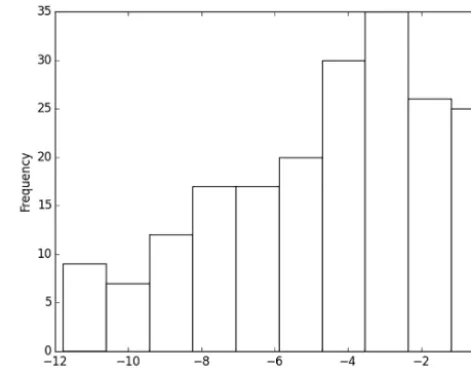
The possibility of performing omnibus tests in MMR re-duces the number of tests from(40×11×6×3)to(40×6)=
240. The individualpvalues are not shown here, but for DB-SCAN their histogram is shown in Fig. 2. Evidently, all of the comparisons yield extremely smallpvalues. At a signif-icance level of 0.05, out of the 240 tests, 53pvalues are not significant when using DBSCAN and 67 are not significant when using GMM. To emphasize the importance of this re-sult, consider the hypothetical situation in which all of these p values were found to be not significant. In that case, no 1Detailed results on clustering are available; they are suppressed
here only to focus on the object-based SA methodology as a whole.
Figure 2.Histogram ofpvalues from the omnibus tests across all days and response variables.
further hypothesis testing would be necessary at all. Indeed, an examination of the individualpvalues displayed in Fig. 2 reveals that a vast majority of the nonsignificant results are associated with the tests when the feature is the eccentricity of an object. As such, one may anticipate that none of the parameters have any effect on eccentricity. The smallness of the remainingpvalues, however, calls for proceeding to the second stage of analysis.
The Bonferroni correction for controlling the FWER re-quires multiplying all of thepvalues by the number of tests (i.e., 240). This correction leads to many more nonsignificant comparisons: 129 for DBSCAN and 111 for GMM. Upon making this correction, in addition to eccentricity some of the other features also emerge as being unaffected by any of the 11 parameters. Further details of these results are presented below. When the Benjamini and Hochberg (1995) procedure is applied to control FDR, the number of nonsignificant com-parisons is similar to those from the uncorrected tests, i.e., 60 for DBSAN and 74 for GMM.
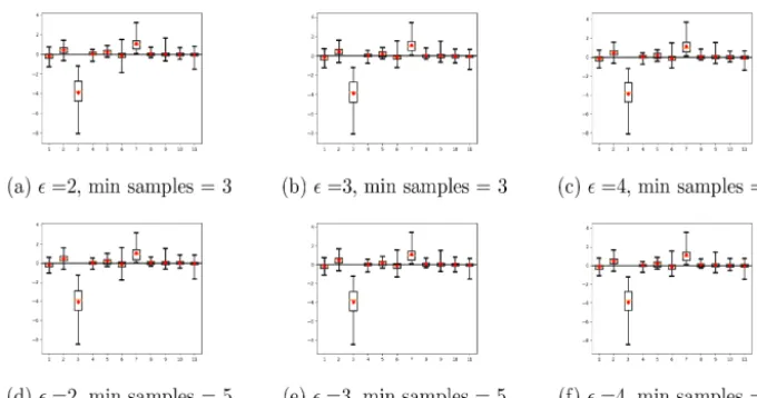
Figure 3.Estimated regression coefficients (i.e., the sensitivity of the model parameters) with median precipitation of the clusters as the response, after clustering with DBSCAN with various parameter values. The red symbols are 95 % simultaneous CIs.
It can also be seen that many of the 11 parameters have a box plot of values mostly around zero. In other words, when considered across multiple days most of the 11 model param-eters have no effect on the median of precipitation. The most obvious exception is parameter 3, which by virtue of having mostly negative values for its regression coefficient is nega-tively associated with median precipitation. Parameter 7 not only has a weaker effect (because the median of the corre-sponding box plot is closer to zero), but it is also not as sta-tistically significant (because zero falls well within the span of the box plot). This parameter is positively associated with precipitation intensity in the typical (median) cluster; i.e., in-creasing the parameter leads to more intense clusters (more details below). The conclusions drawn from an analysis of the CIs in Fig. 3 are the same.
All of these findings are consistent with those found for convective precipitation in Marzban et al. (2014) in which a variance-based sensitivity was performed without any clus-tering at all. This consistency adds justification to the local and/or regression-based SA adopted here, i.e., Eq. (2). It is important to point out that this consistency does not imply that an object-based SA offers nothing more than traditional non-object-based SA; the former assesses the sensitivity of object features, which is something that cannot be done in the latter.
Figure 4 shows the effect of the model parameters on the latitude and longitude of the clusters (top two rows), the amount of precipitation (middle row) in the clusters, and the area and orientation of the clusters (bottom two rows). The three columns correspond to the minimum, median, and max-imum of a feature. Eccentricity has also been examined, but the results are not shown here because it is not affected by any of the 11 parameters; this conclusion is consistent with the results of the omnibus tests performed in the first stage, as mentioned above.
Examination of all of the panels suggests that parameters 4, 5, 8, 9, 10, and 11 have little or no effect on any of the ob-ject features. By contrast, parameters 1, 2, 3, 6, and 7 appear to have varying effects depending on the object feature. Also, the orientation (in addition to the eccentricity) of the clusters is unaffected by any of the parameters.
The strongest effects are from parameters 3 and 7 on the amount of precipitation. This relationship was already exam-ined in Fig. 3, but now the same pattern can be seen in the minimum, median, and maximum intensity (panels g, h, i in Fig. 4), which implies that the effect of parameters 3 and 7 is to shift down and up, respectively, the whole distribution of precipitation intensity.
The next strongest effects are those of parameters 1 and 7 on maximum area (panel l). Given that these two parameters have no effect on the minimum and median area (panels j and k), it follows that these parameters affect only the right tail of the distribution of size. In other words, in contrast to precipitation intensity whose distribution shifts when param-eter 7 is varied, the distribution of size is stretched when that parameter changes. Parameter 6, too, appears to have an ef-fect on maximum area, but to a lesser extent, both statistically and in magnitude.
Whereas parameter 1 tends to stretch out the distribution of area to the right, it appears to have the opposite effect on the minimum and median longitude of the clusters. The effect is weak in magnitude, but statistically significant. It does not affect the maximum longitude (panel f), and so it stretches the distribution of longitude on the left, causing clusters to appear with smaller longitude, which given the encoding of the data used here means to the west. Parameters 2, 6, and 7 appear to have the same effect as parameter 1.
Figure 4.Estimated MMR coefficients (i.e., the sensitivity of the model parameters) on three summary measures (minimum, median, maxi-mum) of different cluster features (latitude, longitude, amount of precipitation, and area and orientation of clusters). Eccentricity is not shown (see text). The red symbols are 95 % simultaneous CIs. The clustering is done with DBSCAN with=2
√
2 and min_samples=3.
maximum latitude, but negatively associated with minimum latitude. In other words, increasing parameter 7 increases the width of the distribution of latitude values, causing them to be more spread out along the latitudes.
All of the above conclusions are based on clustering with DBSCAN with =2
√
2 and min_samples=3. To test the robustness of these results the same analysis was repeated but with GMM as the clustering algorithm and with NC=3. The results (not shown here) are mostly the same. One relatively clear difference between the DBSCAN and GMM results is in the effect of parameters 1 and 7 on area; whereas with DB-SCAN those parameters have an effect only on the maximum area, the results based on GMM suggest a significant effect on all three distribution summary measures (minimum, me-dian, and maximum area).
Further differences between DBSCAN and GMM sensi-tivity results are found when one performs a multivariate test for the effect of the model parameters across all days. For DBSCAN, thepvalues corresponding to each of the six clus-ter features are all found to be nearly zero. So, some of the model parameters do have a significant effect on some of the features. The same is true for GMM, with the exception of latitude and eccentricity for which there is no evidence of an effect (pvalues 0.435 and 0.290, respectively). It may appear that these results are contradictory, but they are not because the respective parameters of the two clustering algorithms have not been tuned to render them comparable. Specifically, the DBSCAN parameters are=2
√
men-tioned earlier, such differences do not point to defects in the methodology; they simply reflect the choice of what the user considers to be an object.
4 Conclusion and discussion
It is shown that by employing methods of cluster analysis and sensitivity analysis one can assess the magnitude and statis-tical significance of the effect of model parameters on the distribution of features (location, intensity, size, and shape) of objects within forecast fields. For example, one can reveal the model parameters that affect the overall location and/or width of the distribution of object features and those that im-pact the shape of the distribution, e.g., by stretching out the left and/or right tail. The approach does not point to any “op-timal” values of the model parameters because that would require optimizing the model parameters to maximize some measure of agreement between forecasts and observations. In other words, although the work here lays the foundation for tuning the model parameters for the purpose of improv-ing forecasts in terms of metrics that arise naturally in spatial verification and evaluation methods, no such tuning is per-formed here.
It is worth pointing out that at least in meteorology, it is not uncommon for different experts to have different notions of an object in the forecast field. As such, the ambiguities dis-cussed above are not specific to clustering algorithms, but are inherent to any object-based approach. In spite of this inher-ent ambiguity, many spatial verification techniques generally rely on some notion of an object. The main reason is that ac-counting for objects in a forecast field is a first step in the verification and evaluation process, and the manner in which objects are defined is of secondary importance.
While this paper is primarily about a methodology, it is worthwhile to provide a possible physical explanation for at least the strongest results in the COAMPS application. The strongest influence or sensitivity is from parameter 3, the fraction of available precipitation fed back to the grid from the Kain–Fritsch scheme. Increasing this fraction reduces convective precipitation and, based on the results in Marzban et al. (2014), increases stable precipitation while not affect-ing total precipitation. It also is responsible for weakenaffect-ing the convective precipitation, i.e., increasing the number of weak systems. The next largest sensitivity is from parameter 7, which controls the temperature difference required to ini-tiate convective precipitation. Again, as shown in Marzban et al. (2014), this parameter also controls a trade-off between convective and stable precipitation and has little effect on to-tal precipitation (along with parameter 1). Parameters 1 and 7 do increase the area of convective precipitation in large precipitation events but not in smaller (areal) precipitation events, likely due to the trade-off between stable and con-vective precipitation in large events such as frontal systems and mesoscale clusters. This process may also explain the
apparent increase in east–west areal coverage and the inten-sification of precipitation events, as found here.
Several generalizations of the proposed methodology are possible. In Marzban et al. (2008) it has been shown that clus-tering can be done not only in the 2-D space of latitude and longitude of each grid point, but also in the 3-D space that includes the amount of precipitation at each grid point. In fact, one may argue that the inclusion of more meteorological quantities in the clustering phase ought to lead to more me-teorologically relevant objects being identified. In turn, this is more likely to lead to a more realistic representation of the effect of the parameters on the object features. The object features may also be extended or revised. For example, here the shape of an object is approximated by an ellipse. But it is possible to use more sophisticated methods of shape analy-sis (Bookstein, 1991; Lack et al., 2010; Micheas et al., 2007; Lakshmanan et al., 2009) to model more complex shapes.
Another possible generalization is to allow for interactions between model parameters. Although the statistical model used here does account for covariance between the model parameters and between the response variables, no explicit interaction is introduced. The inclusion of such terms is straightforward and is unlikely to lead to overfitting, at least in linear models such as MMR.
The use of box plots (in the second stage) to visually dis-play the daily variability of the results is necessarily qualita-tive. But the authors believe that the information provided in the visual display compensates for the lack of rigor accompa-nyingpvalues. CIs are more rigorous than the box plots, but as mentioned previously, that rigor is accompanied by a loss of some information. However, if even more rigor is called for, then it is possible to revise the displays accordingly. For example, one option would be to include a day factor in the MMR model and then test the model parameters. Although the daily variability of theβ coefficients will be lost, each model parameter will be accompanied by ap value. Alter-natively, one may compute Bayesian intervals (Leonard and Hsu, 1999); such intervals are not necessarily symmetric and therefore will be able to convey information on the shape of the underlying sampling distribution. However, they do require additional information, e.g., some knowledge of the prior distribution of theβ values. All of these options will render the analysis more quantitative, although with a differ-ent focus than that emphasized here.2
Code and data availability. The code and the data analyzed here occupy about 4.0G of computer space and are avail-able upon request from the corresponding author or from https://doi.org/10.5281/zenodo.1043542.
2The authors acknowledge an anonymous reviewer for these
Competing interests. The authors declare that they have no conflict of interest.
Acknowledgements. This work has received support from the Office of Naval Research (N00014-12-G-0078 task 29) and the National Science Foundation (AGS-1402895). The authors are grateful to James D. Doyle and Nicholas C. Lederer for providing invaluable support. Ethan P. Marzban is acknowledged for making the flowchart in Fig. 1.
Edited by: Paul Ullrich
Reviewed by: three anonymous referees
References
Ahijevych, D., Gilleland, D. E., Brown, B. G., and Ebert, E. E.: Ap-plication of spatial verification methods to idealized and NWP-gridded precipitation forecasts, Weather Forecast., 24, 1485– 1497, 2009.
Backman, J., Wood, C. R., Auvinen, M., Kangas, L., Han-nuniemi, H., Karppinen, A., and Kukkonen, J.: Sensitivity anysis of the meteorological preprocessor MPP-FMI 3.0 using al-gorithmic differentiation, Geosci. Model Dev., 10, 3793–3803, https://doi.org/10.5194/gmd-10-3793-2017, 2017.
Baldwin, M. E., Lakshmivarahan, S., and Kain, J. S.: Verification of mesoscale features in NWP models, in: 9th Conf. on Mesoscale Processes, Amer Meteor. Soc., Ft. Lauderdale, FL, 255–258, 2001.
Baldwin, M. E., Lakshmivarahan, S., and Kain, J. S.: Development of an “events-oriented” approach to forecast verification, in: 15th Conf. Numerical Weather Prediction, San Antonio, TX, 2002. Banfield, J. D. and Raftery, A. E.: Model-based Gaussian and
non-Gaussian clustering, Biometrics, 49, 803–821, 1993.
Benjamini, Y. and Hochberg, Y.: Controlling the false discovery rate: a practical and powerful approach to multiple testing, J. R. Stat. Soc., B 57, 289–300, 1995.
Bolado-Lavin, R. and Badea, A. C.: Review of sensitivity analysis methods and experience for geological disposal of radioactive waste and spent nuclear fuel, JRC Scientific and Technical Re-port, available at: https://core.ac.uk/download/pdf/38614334.pdf (last access: 18 April 2018), 2008.
Bookstein, F. L.: Morphometric Tools for Landmark Data: Geome-try and Biology, Cambridge University Press Cambridge, 1991. Bretz, F., Hothorn, T., and Westfall, P.: Multiple Comparisons Using
R, Chapman and Hall, 2001.
Brown, B. G., Mahoney, J. L., Davis, C. A., Bullock, R., and Mueller, C.: Improved approaches for measuring the quality of convective weather forecasts, in: 16th Conference on Probability and Statistics in the Atmospheric Sciences, Orlando, FL, 20–25, 2002.
Casati, B., Ross, G., and Stephenson, D.: A new intensity-scale ap-proach for the verification of spatial precipitation forecasts, Me-teorol. Appl., 11, 141–154, 2004.
Cioppa, T. and Lucas, T.: Efficient nearly orthogonal and space-filling latin hypercubes, Technometrics, 49, 45–55, 2007. Davis, C., Brown, B., and Bullock, R.: Object-based verification
of precipitation forecasts, Part I: Methodology and application
to mesoscale rain areas, Mon. Weather Rev., 134, 1772–1784, 2006a.
Davis, C. A., Brown, B., and Bullock, R.: Object-based verification of precipitation forecasts. Part II: Application to convective rain systems, Mon. Weather Rev., 134, 1785–1795, 2006b.
DelSole, T. and Yang, X.: Field Significance of Regression Patterns, J. Climate, 24, 5094–5107, 2011.
Dmitrienko, A., Tamhane, A. C., and Bretz, F. (Eds.): Multiple Test-ing Problems in Pharmaceutical Statistics, Chapman and Hall, 2009.
Doyle, J. D., Jiang, Q., Smith, R. B., and Grubiši´c, V.: Three-dimensional characteristics of stratospheric mountain waves dur-ing T-REX, Mon. Weather Rev., 139, 3–23, 2011.
Du, J. and Mullen, S. L.: Removal of Distortion Error from an En-semble Forecast, Mon. Weather Rev., 128, 3347–3351, 2000. Ebert, E.: Fuzzy verification of high-resolution gridded forecasts:
a review and proposed framework, Meteorol. Appl., 15, 51–64, 2008.
Ebert, E. E. and McBride, J. L.: Verification of precipitation in weather systems: determination of systematic errors, J. Hydrol-ogy, 239, 179–202, 2000.
Errico, R. M.: What is an Adjoint Model?, B. Am. Meteorol. Soc., 78, 2577–2591, 1997.
Ester, M., Kriegel, H.-P., Sander, J., and Xu, X.: A density-based algorithm for discovering clusters in large spatial databases with noise, in: Proceedings of Knowledge Discovery and Data Mining (KDD-96), 96, 226–231, 1996.
Everitt, B. S.: Cluster Analysis, Heinemann Educational Books, London, 1980.
Fox, J., Friendly, M., and Weisberg, S.: Hypothesis tests for multi-variate linear models using the car package, R. J., 5, 39–52, 2013. Fraley, C. and Raftery, A.: Model-Based Clustering, Discriminant Analysis, and Density Estimation, J. Am. Stat. Assoc., 97, 611– 631, 2002.
French, S., Lekic, V., and Romanowicz, B.: Waveform Tomography Reveals Channeled Flow at the Base of the Oceanic Astheno-sphere, Science, 342, 227–230, 2013.
Froyland, G., Stuart, R. M., and van Sebille, E.: How well-connected is the surface of the global ocean?, Chaos, 24, 033126, https://doi.org/10.1063/1.4892530, 2014.
Gilleland, D. E., Ahijevych, D., Brown, B. G., Casati, B., and Ebert, E. E.: Intercomparison of Spatial Forecast Verification Methods, Weather Forecast., 24, 1416–1430, 2009.
Hacker, J. P., Snyder, C., Ha, S.-Y., and Pocernich, M.: Linear and non-linear response to parameter variations in a mesoscale model, Tellus A, 63, 429–444, https://doi.org/10.1111/j.1600-0870.2010.00505.x, 2011.
Hodur, R. M.: The Naval Research Laboratory’s Coupled Ocean/Atmosphere Mesoscale Prediction System (COAMPS), Mon. Weather Rev., 125, 1414–1430, 1997.
Hoffman, R. N., Liu, Z., Louis, J.-F., and Grassotti, C.: Distortion representation of forecast errors, Mon. Weather Rev., 123, 2758– 2770, 1995.
Jiang, Q. and Doyle, J. D.: The impact of moisture on Mountain Waves, Mon. Weather Rev., 137, 3888–3906, 2009.
Kalra, T. S., Aretxabaleta, A., Seshadri, P., Ganju, N. K., and Beudin, A.: Sensitivity analysis of a coupled hydrodynamic-vegetation model using the effectively subsampled quadratures method (ESQM v5.2), Geosci. Model Dev., 10, 4511–4523, https://doi.org/10.5194/gmd-10-4511-2017, 2017.
Keil, C. and Craig, G. C.: A displacement-based error measure ap-plied in a Regional Ensemble Forecasting System, Mon. Weather Rev., 135, 3248–3259, 2007.
Lack, S. A., Limpert, G. L., and Fox, N. I.: An object-oriented mul-tiscale verification scheme, Weather Forecast., 25, 79–92, 2010. Laine, M., Solonen, A., Haario, H., and Järvinen, H.: Ensemble
pre-diction and parameter estimation system: the method, Q. J. Roy. Meteor. Soc, 138, 289–297, 2012.
Lakshmanan, V. and Kain, J. S.: A Gaussian Mixture Model Ap-proach to Forecast Verification, Weather Forecast., 25, 908–920, 2010.
Lakshmanan, V., Hondl, K., and Rabin, R.: An Efficient, general-purpose technique for identifying storm cells in geospatial im-age, J. Atmos. Ocean. Tech., 26, 523–537, 2009.
Leonard, T. and Hsu, J. S. J.: Bayesian Methods; An Analysis for Statisticians and Interdisciplinary Researchers, Cambridge Uni-versity Press, Cambridge, 1999.
Li, J., Hsu, K., AghaKouchak, A., and Sorooshian, S.: An object-based approach for verification of precipitation estimation, Int. J. Remote Sens., 36, 513–529, 2015.
Li, X., Sudarsanam, N., and Frey, D. D.: Regularities in data from factorial experiments, Complexity, 11, 32–45, 2006.
Lorenz, E. N.: Deterministic non-periodic flow, J. Atmos. Sci., 20, 130–141, 1963.
Lucas, D. D., Klein, R., Tannahill, J., Ivanova, D., Brandon, S., Domyancic, D., and Zhang, Y.: Failure analysis of parameter-induced simulation crashes in climate models, Geosci. Model Dev., 6, 1157–1171, https://doi.org/10.5194/gmd-6-1157-2013, 2013.
Marzban, C.: Variance-based Sensitivity Analysis: An illustration on the Lorenz ’63 model, Mon. Weather Rev., 141, 4069–4079, 2013.
Marzban, C. and Sandgathe, S.: Cluster analysis for verification of precipitation fields, Weather Forecast., 21, 824–838, 2006. Marzban, C. and Sandgathe, S.: Cluster Analysis for
Object-Oriented Verification of Fields: A Variation, Mon. Weather Rev., 136, 1013–1025, 2008.
Marzban, C., Sandgathe, S., and Lyons, H.: An Object-oriented Ver-ification of Three NWP Model Formulations via Cluster Analy-sis: An objective and a subjective analysis, Mon. Weather Rev., 136, 3392–3407, 2008.
Marzban, C., Sandgathe, S., Lyons, H., and Lederer, N.: Three Spa-tial Verification Techniques: Cluster Analysis, Variogram, and Optical Flow, Weather Forecast., 24, 1457–1471, 2009. Marzban, C., Sandgathe, S., Doyle, J. D., and Lederer, N. C.:
Variance-Based Sensitivity Analysis: Preliminary Results in COAMPS, Mon. Weather Rev., 142, 2028–2042, 2014. McLachlan, G. J. and Peel, D.: Finite Mixture Models, John Wiley
& Sons, Hoboken, NJ, USA, 2000.
Micheas, A. C., Fox, N. I., Lack, S. A., and Wikle, C. K.: Cell iden-tification and verification of QPF ensembles using shape analysis techniques, J. Hydrol., 343, 105–116, 2007.
Montgomery, D. C.: Design and Analysis of Experiments, Wiley & Sons, 7th edn., 2009.
Nachamkin, J. E.: Mesoscale verification using meteorological composites, Mon. Weather Rev., 132, 941–955, 2004.
Ollinaho, P., Järvinen, H., Bauer, P., Laine, M., Bechtold, P., Susilu-oto, J., and Haario, H.: Optimization of NWP model closure pa-rameters using total energy norm of forecast error as a target, Geosci. Model Dev., 7, 1889–1900, https://doi.org/10.5194/gmd-7-1889-2014, 2014.
Rencher, A. C. and Christensen, W. F.: Methods of Multivari-ate Analysis, John Wiley & Sons, Inc., Hoboken, NJ, USA, https://doi.org/10.1002/9781118391686.ch10, 2012.
Roberts, N. M. and Lean, H. W.: Scale-Selective Verification of Rainfall Accumulations from High-Resolution Forecasts of Con-vective Events, Mon. Weather Rev., 136, 78–97, 2008.
Robock, A., Luo, L., Wood, E. F., Wen, F., Mitchell, K. E., Houser, P., Schaake, J. C., Lohmann, D., Cosgrove, B., Sheffield, J., Duan, Q., Higgins, R. W., Pinker, R. T., Tarpley, J. D., Basara, J. B., and Crawford, K. C.: Evaluation of the North American Land Data Assimilation System over the southern Great Plains during warm seasons, J. Geophys. Res., 108, 8846–8867, 2003. Roebber, P.: The role of surface heat and Moisture Fluxes
Associ-ated with large-scale ocean current meanders in maritime cyclo-genesis, Mon. Weather Rev., 117, 1676–1694, 1989.
Roebber, P. and Bosart, L.: The sensitivity of precipitation to cir-culation details, part i: an analysis of regional analogs, Mon. Weather Rev., 126, 437–455, 1989.
Rosenblatt, J.: A practioner’s guide to multiple hypothesis test-ing error rates, Cornell University Library, arXiv:1304.4920v3, 2013.
Safta, C., Ricciuto, D. M., Sargsyan, K., Debusschere, B., Najm, H. N., Williams, M., and Thornton, P. E.: Global sensitivity anal-ysis, probabilistic calibration, and predictive assessment for the data assimilation linked ecosystem carbon model, Geosci. Model Dev., 8, 1899–1918, https://doi.org/10.5194/gmd-8-1899-2015, 2015.
Saltelli, A., Ratto, M., Andres, T., Campolongo, F., Cariboni, J., Saisana, M., and Tarantola, S.: Global Sensitivity Analysis: The Primer, Wiley Publishing, 2008.
Saltelli, A., Annoni, P., Azzini, I., Campolongo, F., Ratto, M., and Tarantola, S.: Variance based sensitivity analysis of model out-put: Design and estimator for the total sensitivity index, Comput. Phys. Commun., 181, 259–270, 2010.
Samsel, F., Petersen, M., Abram, G., Turton, T. L., Rogers, D., and Ahrens, J.: Visualization of Ocean Currents and Eddies in a High-Resolution Global Ocean-Climate Model, in: Proceedings of the 15th International Conference for High Performance Com-puting, Networking, Storage and Analysis, Austin, TX, 2015. Stein, A. F., Draxler, R. R., Rolph, G. D., Stunder, B. J. B., Cohen,
M. D., and Ngan, F.: NOAA’S HYSPLIT Atmospheric Transport and Dispersion Modeling System, B. Am. Meteorol. Soc., 96, 2059–2077, 2015.
Venugopal, V., Basu, S., and Foufoula-Georgiou, E.: A new metric for comparing precipitation patterns with an applica-tion to ensemble forecasts, J. Geophys. Res., 110, D08111, https://doi.org/10.1029/2004JD005395, 2005.
Multi-Temporal Satellite Imagery and Ancillary Data, IEEE J. Sel. Top. Appl., 4, 252–264, 2011.
Wang, Y. H., Fan, C. R., Zhang, J., Niu, T., Zhang, S., and Jiang, J. R.: Forecast Verification and Visualization based on Gaussian Mixture Model Co-estimation, Comput. Graph. Forum, 34, 99– 110, 2015.
Wealands, S. R., Grayson, R. B., and Walker, J. P.: Quantitative comparison of spatial fields for hydrological model assessment: some promising approaches, Adv. Water Resour., 28, 15–32, 2005.
Wernli, H., Paulat, M., Hagen, M., and Frei, C.: SAL – A Novel Quality Measure for the Verification of Quantitative Precipitation Forecasts, Mon. Weather Rev., 136, 4470–4487, 2008.
Wilks, D. S.: Statistical Methods in the Atmospheric Sciences, 3rd edn., Elsevier Inc., 2011.